February, 2003
The E
ff
ects of Government De
fi
cit on Equilibrium
Real Exchange Rates and Stock Prices
Abstract
This paper studies the effect of government deficits on equilibrium real exchange rates and stock prices. The theoretical part modifies a two-country cash-in-advance model like used in Lucas(1982) and Sar-gent(1987) in order to accommodate an exchange rate market and a government that pursues fiscal and monetary policy targets. The implied result is that unanticipated shocks in government deficits raise expectations of both taxes and inflation and, therefore, are associated with real exchange rate devalua-tions and lower stock prices. Thisfinding is strongly supported by empirical evidence for a group of 19 countries, representing 76% of world production.
Marcelo Moura Ibmec Business School São Paulo - SP, Brazil
E-mail: [email protected] - Tel: 55-11-3175-2313 / 55-11-3175-2300 ext. 113 Fax:11-55-3175-2315 JEL: F41, F47, H30, H60
1
Introduction
Can persistent government budget deficits affect the exchange rate value? What are the possible links between fiscal and monetary policies and stock market performance? Given some recent currency crises and the increasing intensity of capital mobility since the early 70’s, when almost only institutional funds were available, these questions represent an increasing concern among policymakers and academics.1 Still, until recently economists made little effort to link government
fiscal solvency to the exchange rate value and other asset prices. The present paper aims to contribute towardfilling this gap.
This study is theoretical and empirical. The theoretical part, which constitutes the next section, develops a model where government deficits influence supply and demand, and therefore prices, for the national currency exchange rate and stocks. The empirical part, presented in section 3, uses post Bretton Woods data for 19 countries in order to study the empirical evidence relating asset price movements tofiscal fundamentals.
The sample is representative in terms of world production and includes both industrialized and emerging economies. The inclusion of developing economies in the sample is important be-cause it allows one to test the usual claim that developing economies are more vulnerable than industrialized countries to currency and stock markets crises resulting from fiscal shocks.
The economic model’s main contribution is to link a government policy, of pursuing specific targets for money expansion and taxes, to private agents ’ expectations about future taxes and inflation. More specifically, given the government goals, what matters is how agents expect the government tofinance an increase in the government budget deficit: by an increase in the public debt, and consequently higher taxes in the future, or by money creation.2
1 To name a few up to the time this paper was written: Sweden 1992, see Obstfeld (1994); Mexico
1995, see Cole and Kehoe (1996); Southeast Asian economies 1997, see Burnside, Eichenbaum and Rebelo (1998); Russia 1998 and Brazil 1999, for data on the last two see IMF, International Financial Statistics CD-ROM.
2Another possibility would be government explicit default; for the sake of simplicity I will assume that
If agents expect that an increase in the government debt willfinance the deficit, they anticipate higher taxes in the future and lower net dividends from taxable assets, which means lower stock prices today. On the other hand, when private agents expect that money creation will be used as thefinancing instrument, they anticipate future inflation, which in the model implies exchange rate devaluation. On a more general level, households attribute a positive probability to each possible event. Therefore, an unexpected increase in the deficit raises expectations for future taxes and future inflation, implying lower stock prices and exchange rate devaluation.
The model also introduces an exchange currency market at the end of the day. In this market, currency’s demand and supply determines the equilibrium real exchange rate. This price deter-mination reflects the relative inflation risk of each country, which depends onfiscal fundamentals. This results in a more general form of no-arbitrage conditions than the Power Purchasing Parity (PPP) theory. The PPP theory would be a specific case where there is no inflation risk, or the same relative risk, in carrying each currency overnight.
Section 3 explores the empirical data. Data is annual and represents 19 countries during the post Bretton-Woods period, 1974-98. The results give empirical support to the model developed in section 2. Pooled data regressions demonstrate a statistically significant correlation between real exchange rates and stock market prices, on the one hand, and the government budget deficit and otherfiscal fundamentals on the other hand. The section also estimates the equilibrium exchange rate equation from the previous section. Using only data on government budget deficits and debt, the artificial time series approximates very closely the actual exchange rates.
Section 4 gathers the results from the previous chapters and presents the paper’sfinal conclu-sions and directions for future research.
2
Fiscal Fundamentals and Asset Pricing
The goal of this section is twofold: first, to review the literature concerning the effects of gov-ernment budget deficits on the economy and to discuss the empirical evidence on the topic; and second, to develop an economic model that constructs a more direct link betweenfiscal policy and asset prices.
The next section presents the review of the literature. Section 2.2 explores some preliminary empirical evidence, which will be studied in more detail in section 3. Section 2.3 introduces some modifications on Lucas ’ (1982) and Sargent’s (1987) two-country cash-in-advance models, in order to link exchange rates and stock prices tofiscal fundamentals. Section 2.4 extends the model to a small economy where there is no aggregate risk.
2.1
Review of the Literature
Standard economic theory usually predicts that an increase in the government deficit will attract foreign capital and appreciate the equilibrium exchange rate, provided that the government has no problem rolling over its debt.
For instance, Ball and Mankiw (1995) claim that a higher government deficit increases the demand for loans, which drives interest rates up and attracts foreign capital. By equilibrium of the balance of payments, the counterpart to the foreign capitalflow is a decrease in the commercial account surplus, which requires a real exchange rate appreciation.
Despite the simplicity and the logical appeal of this argument, it is in one sense just a ma-nipulation of account identities. Namely, the gross domestic product, GDP, can be decomposed as:
whereYtis theGDP,Ctis private consumption,Gtis the government consumption,Itis invest-ment and Xt and Mt are respectively exports and imports of goods and services. Subtracting taxes,Tt, from both sides and rearranging yields
(Tt−Gt) + (Yt−Tt−Ct) + (Mt−Xt) =It (2.1.2)
Ball and Mankiw (1995) claim that an decrease in government surplus (Tt−Gt), causes an decrease in private savings (Yt−Tt−Ct), and investment It which are altogether offset by an increase in external savings (Mt−Xt)such that equation (2.1.2) is valid.
However, the opposite result can be obtained as well, everything depending crucially on the private agent’s demand for government bonds. For instance, if the government cannot credibly guarantee higher surpluses in the future to repay debt, agents may be unwilling to acquire more bonds. The increase in the interest rate may be unable to increase the demand for bonds because it worsens thefiscal situation even more. Private agents will anticipate higher inflation, or a public default, or higher taxes in the future, which leads to capital flight, currency devaluation, and a fall in stock prices. Notice that, according to equation (2.1.2), investment level falls sufficiently to accommodate decreases in all of the three terms on the right hand side.
Sargent and Wallace (1981) show that demand for bonds has importantfiscal and monetary policy effects. The authors assert that the real stock of bonds cannot indefinitely grow faster than the size of the economy. Thus, the demand for bonds will place an upper limit on the ratio of government debt to GDP and once this limit is reached, government deficits will have to be
government deficit but also due to the tax base cut resulting from capitalflight. In equilibrium, all investors will take their capital abroad. Obstfeld (1994) explores a self-fulfilling model of currency crises where government endogenous responses to market expectations and fiscal fundamentals play an active role in determining the equilibrium exchange rate.
Despite the possibility offiscal shocks generating currency crises, the literature on speculative attacks of fixed exchange rate regimes gives little attention to those fundamentals. Garber and Svensson (1995) survey the literature and report that, although many of its models link the occurrence of speculative attacks to the increase of domestic credit, researchers give little attention to the relation between governmentfinancial needs and the creation of domestic credit.
In summary, the discussion above demonstrates that the government’s ability to roll over its debt, and private agent’s expectations about government’sfinancing strategies, mediate the effects of budget deficits on the economy. However, the main theories of equilibrium exchange rates ignore the role offiscal fundamentals. Subsection 2.2.1 reviews equilibrium exchange rate theories while subsection 2.2.2 discusses asset pricing equations and fiscal policies.
2.1.1 Equilibrium Exchange Rates
Most of the macroeconomic models that try to capture exchange rate movements assume that Power Purchasing Theory (PPP) theory of exchange rate determination holds. As stated by Dornbusch (1995, page 265): The PPP theory “asserts (in its most common form) that the exchange rate between two currencies over any period of time is determined by the change in the two countries relative prices levels.” This is also known as the weak formof thePPP theory.
Despite the simplicity and no-arbitrage appeal of thePPP theory, empirical evidence shows that it does not hold on the short run. Froot and Rogoff (1995) survey the extensive literature testing the PPP hypothesis and report that half-life deviations from PPP are around 3-5 years for major industrialized countries.3
3 Killian and Zha (1999) using a Bayesian approachfind evidence of even higher half-lives for major
Sjaastad (1996, 1998, 1998b and 1999) provides one remarkable explanation for the empirical failure of the PPP theory. While one could argue that prices of traded goods are determined by world demand and supply, the price of a nontraded good does not have to be the same for different countries.
Therefore, a more appropriate definition of the real exchange rate consists of the ratio of a price index for traded goods to a price index for nontraded goods measured in a common numeraire, the true real exchange rate. Sjaastad’s methodology also shows that the use of the conventional measure ofPPP-real exchange rate as an empirical proxy of thetrue-real exchange rate is subject to very high measurement error and sheds doubt on the relevance of a plethora of papers testing thePPP hypothesis.
One example of the use of thePPP theory on economic models is the seminal paper of Lucas (1982), which integrates monetary theory with the apparatus of modern financial economics. In his model, provided symmetric allocation between agents, the real exchange rate is the ratio of the marginal utilities for foreign and domestic consumption goods. Consequently, an increase in government purchases implies change in the marginal utilities ratio and movements on the real exchange rate.
The Fiscal Theory of the Price Level (FTP) [see Cochrane (1998, 1999, 2000) and Woodford (1996)] inspires a different approach that tries to linkfiscal fundamentals to the real equilibrium exchange rate. Dupor (2000) and Loyo (1998) extend theFTP to open economies and obtain an indeterminacy in the equilibrium exchange rate, similar to the classical result obtained by Kareken and Wallace (1981).
debt plus money supply to the discounted value of future surpluses.
2.1.2 Stock Prices
Consider an asset that produces a stochastic flow of dividends{Dt+j}+j=0∞, which is taxed at the
ad-valorem rate{τt+j}+j=0∞.Since the netflow of dividends is{(1−τt+j)Dt+j}+j=0∞,this asset will
be priced at
ps t=
+P∞
j=0
Et[mt,t+j(1−τt+j)Dt+j] (2.1.3)
where mt,t+j is the stochastic discount factor from periodttot+j.
From this pricing equation it is trivial to see that thefiscal policy on government taxes will have direct effects on asset prices. If, for simplicity, we assume that there are no aggregate risks such that the discount factor does not depend on government variables, then it is easy to verify from equation (2.1.3) that higher taxation implies lower stock prices. There would be no effect only if taxes are not linked to stock ownership, as in the case of lump-sum taxes.
In the consumption-capital pricing model (C-CAPM), pioneered by, among others, Lucas ’ (1978) tree-model, we have mt,t+j = βj[u0(Ct+j)/u0(Ct)], where β ∈ (0,1) is the intertemporal discount rate andu0(C
s)denotes the representative agent one-period marginal utility of consuming
Cs at time periods(by equilibrium of the goods marketYt+j =Gt+j+Ct+j, whereYt+j is the national income andGt+jthe government consumption). Thus, for theC-CAPM equation (2.1.3) specializes to
pst=+P∞ j=0
Et
" βju0(Y
t+j−Gt+j)
u0(Y
t−Gt)
(1−τt+j)Dt+j
#
(2.1.4) For theC−CAP M model, not only the way that governmentfinances its expenditures but also the government consumption stream, {Gt+j}+j=0∞, influences stock prices. The model to be
2.2
Empirical Motivation
The review of the literature showed that the effects of budget deficits rely on the assumptions made about the government’s ability to roll over its debt. If higher interest rates attract foreign capital to finance an increase in government deficit, the exchange rate should appreciate. On the other hand, if an increase in government deficit generates fears of higher future inflation, or higher taxes, or even explicit defaults, the expected result could be capitalflights, currency devaluation, and lower stock prices.
Some can argue that confidence crises or “hard landing scenarios” are more relevant for devel-oping economies but not really the case for industrialized countries. However, some industrialized countries can show even more volatility on exchange rates than emerging economies.4
Section 2.1.2 showed that stock prices depend on the expected level of future government purchases and future taxes. Therefore, since “hard landing scenarios” are usually associated with changes infiscal policy, these confidence crises can also create substantial stock price movements. This section sheds more light on the discussion introducing preliminary empirical evidence related to asset prices and government deficits.5
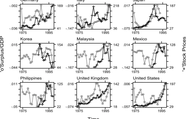
Figure 1 plots the government budget deficit, as a ratio of GDP, and the real exchange rate for a selected group of economies.6 The plots present strong empirical evidence in support of a government deficit being positively correlated with real exchange rate devaluations.
4Indeed, exchange rates of developed economies can show even more volatility than exchange rates of
developing economies. Edwards and Savastano (1999) report that during the period of January 1995 to November 1997, when the Mexican Peso floated against the dollar without explicit interventions of the Mexican Central Bank, the Mexican Peso/US dollar exchange rate was less volatile than the Yen, the Deutsche Mark, and the Pound/ Dollar exchange rates.
5A more complete analysis of the empirical evidence concerningfiscal policy and asset pricing, including
a detailed descriptions of the data used, is discussed in section 3.
6The Real Exchange Rate is defined ase
tPtU S/PtN at.whereet is the nominal exchange rate in terms of
national currency per US dollars at timet,PU S
t and isPtN at. are respectively the price level at timetof
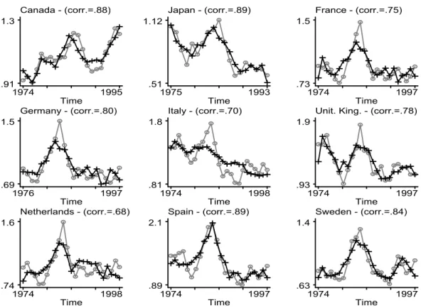
Figure 2 plots government surpluses, as a ratio of GDP, and stock prices.7 The sample includes
five industrialized economies: United States, Japan, Germany, Italy, and the United Kingdom, and four emerging economies: Mexico, South Korea, Malaysia, and the Philippines.
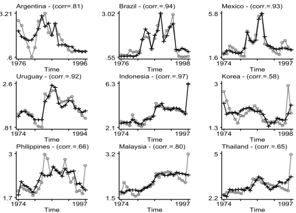
The data presented in Figures 1 and 2 indicate a positive correlation between government surpluses and stock prices values for all the countries analyzed. The empirical evidence of Figure 2 can be explained in light of the asset pricing equation (2.1.3) and the consumption-based (C-CAPM) model, equation (2.1.4). The intuition is that an unexpected higher government deficit (or surplus) can indicate expectations of higher (or lower) taxes and higher (or lower) inflation in the future and, consequently by (2.1.3) or (2.1.4), lower (or higher) stock prices.
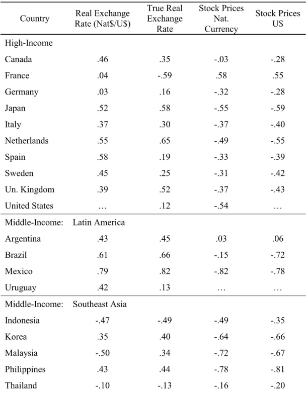
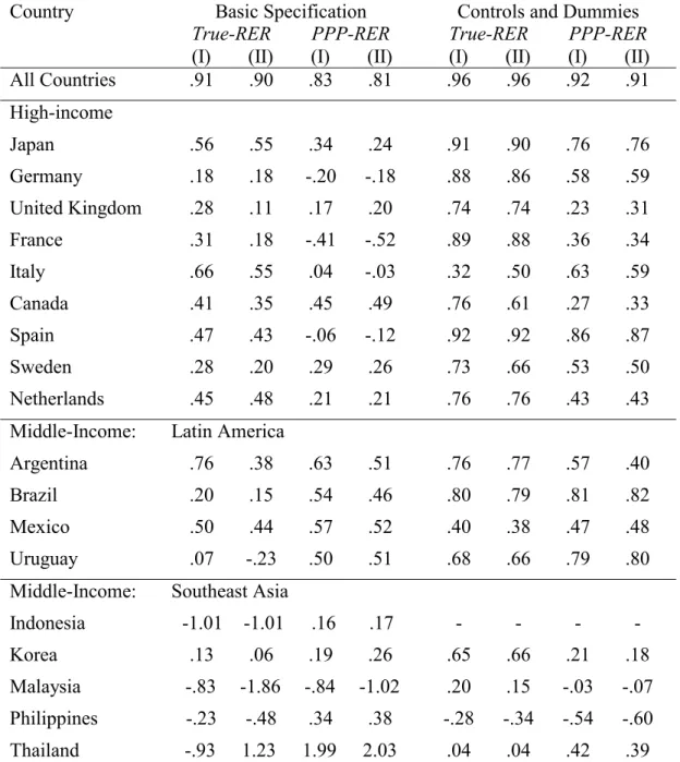
Table 1 expands the sample used in Figures 1 and 2, reporting the sample correlations of government budget deficit as a ratio of GDP with thetrue and thePPP real exchange definitions and stock prices measured in 1995 national currency and 1995 U$ values.8
Data on Table 1 is annual and it is distributed in an unbalanced way for the post Bretton-Woods period, 1974-1998. The sample includes 10 high income economies and 9 middle income economies.9 These countries responded for a total GDP of U$21,957 billions in 1998, which represents 76% of world total production.
Looking at table 1 we can verify that all high-income economies, excluding France, present evidence of a positive correlation of government financial requirements with exchange rate deval-uation and lower stock prices.
The Latin America middle-income economies also demonstrate currency devaluations associ-ated with higher deficits. However, the same evidence is not so clear for emerging Southeast Asian
7 In Figure 1 annual stock prices are from DataStream Primark total market index, which is a price
index for the most important stocks of each country. Stock prices are end of period values measured in national currency and deflated for 1995 values. The 1995 values are also normalized to 100.
8The methodology to compute the true real exchange rates is the same as described in Sjaastad (1996,
1998, 1998b and 1998), see appendix D. The PPP real exchange rate definition is the conventional one, nominal exchange rate times relative price levels. Stock prices are measured in constant currency values from 1995. A more detailed description of the data used in this section is presented in subsection 3.1.
9 Definitions follow the World Bank classification as of 1998. High Income Economies correspond to
economies.
For stock market correlations with government deficits, the only exception to a negative corre-lation between deficits and stock prices seems to be Argentina. In general, the empirical evidence for the selected sample of 19 countries is coherent with the intuition that increases in government deficit imply expectations of higher inflation and higher taxes in the future, devaluing the national currency value and depressing stock prices.
The model developed in the next section will explore this insight to match the empirical observations. Section 3 will investigate in more detail the empirical evidence controlling for known effects in the literature.
2.3
A Two-Country Cash-in-Advance Model
Consider a world economy that consists of two countries denoted by Home, H, and Foreign, F, each with its own currency, respectively denoted byH$andF$. Private agents of these economies are characterized by one representative agent (Household) for each country. As in Lucas (1978), there is one good, which is produced by trees. Each country indexed byj, where j=H, F, has one tree that produces at time t a total amount of Ytj units of this consumption good. For the sake of simplicity, the endowment of countryj is supposed to grow at a deterministic rateγj
Ytj = (1 +γj)tY0j (2.3.1)
Households in both countries have identical preferences represented by the utility function
E0
·+∞ P
t=0
βt(c
H
it +cFit)1−σ−1 1−σ
¸
(2.3.2)
where cjit denotes the consumption of goods produced in country j by the Household residing in countryi.
If the Household resident in countryiheld, at the end of periodt, sji,t shares of stocksj, j=H, F, the amount of tax due in periodt,measured inj$, issitjτtYtjPtj.
The government of countryj issues government bonds, prints the national currency, and col-lects taxes from the ownership of their respective country’s stock in order to finance expendi-ture levels of gtjYtj units of goods. We shall assume that the level of government purchases,
xt= (gtH, gtF), is governed by afirst-order Markov Process, in particular, assume forj =H, F:
gjt = (¯gj+εtj+εjt−1) (2.3.3)
where the innovations are such that
εjt˜U[−hj,+hj], hj >0, ¯gj±2hj∈(0,1) ∀t, j (2.3.4)
Equations (2.3.3) and (2.3.4) assume that government purchases have some persistence and do not exceed the level of national production. The argument for government expenditures following (2.3.3) is that a high deficit (or surplus) will more likely be followed by a high deficit (or surplus) again in the next period.
In order to simplify the argument, assume that the entire government debt consists of one-period inflation indexed bonds. Denote the price level, measured inj$ currency,for the consump-tion good in countryj byPtj. Thus, at the beginning of periodt, countryj0sgovernment spends (1 +rt)PtjBjt to repay debt acquired in period t−1, and collects PtjBtj+1 by issuing new debt
and by redeeming τjtYtjPtj from taxes. An extra source of revenue for the government of country j comes from seignorage revenues, which generates at timetan additional amount ofMtj+1−Mtj
in j$.
In units of consumption goods, governmentj0sis subject to the budget constraint
Bjt+1+τjtYtj+M j
t+1−Mtj
Ptj = (1 +r
j
output cannot have an explosive path, equation (2.3.5) can be written in an integrated form as
bjt+1=+P∞ k=1
Et
"
k
Q
l=1
µ
1 +γj
1 +rt+l
¶ Ã
τjt+k−gtj+k+ µ j t+k 1 +µjt+k
!#
(2.3.6)
where bjt+1≡Btj+1/Ytj is the end of period debt as a ratio of GDP andµjt≡Mtj+1/Mtj−1is the growth rate of money supply.
As in Sargent (1987), governments have to set aside enough cash to buy consumption goods. Therefore, the amount of cash that governmentjholds,mjt,after collecting taxes and rolling over its debt has to satisfy10
mgjt ≥PtjgjtYtj (2.3.7)
Because government debt is inflation-indexed and there is no default risk, no-arbitrage implies that the real interest rate has to be the same in both countries, that is
rtH=rFt =rt (2.3.8)
A f iscal policy for the government j at time period t is defined as a choice of tax sequence
{τjt+k}k+=0∞ . A monetary policy for the government j at time periodt is defined by a sequence of money supplies {Mtj+1+k}+k=0∞. Given the stochastic sequences for interest rates, government expenditures, and national endowment{rt+k, gHt+k, gtF+k, YtH+k, YtF+k}+k=0∞,af easible policyfor
gov-ernment j at time period t is a sequence offiscal and monetary policies, possibly contingent on the state of the economyxt= (gtH, gtF), such that equations (2.3.3) to (2.3.8) hold.
The structure of trading plays a very important role in the model.11 At the beginning of each period, information is revealed and the values of the variables gjt, τjt, Mtj+1, Ptj forj =H, F
are announced, as well as the contingent futurefiscal and monetary policies of both governments,
{τjt+k, Mtj+1+k}+k=1∞ forj =H, F. Afterward, the time period is subdivided in three distinct and consecutive trading sections: the securities trading section, theshopping section, andfinally the currency trading section.
1 0This amount will bemgj
t =PtjτjtYtj+PtjBtj+1−(1 +r
j
t)PtjBjt+Mtj+1−M
j t.
The securities trading section is divided into two distinct sections, one for each country. In country j’s securities trading section, private agents of both countries trade only government’s j bonds, j$ currency, and countryj’s stock shares. During these sections, the country j govern-ment repays old debt, issues new debt, and at the end of the section collects taxes in cash from stockholders.
During the trading section being held in countryj,the Household residing in countryi chooses the amount of currency to take to the shopping section, mpjit, the amount of government j bonds to take to the next period,Bji,t+1, and the number of stock shares from trees located on country j to be carried over to periodt+1. The Household shall face the budget constraint
mpjit Ptj +B
j
i,t+1+sjitτjtYtj+sjitqtj≤θjit (2.3.9) where qjt is the spot price for countryj stocks,sjitτjtYtj is the amount of taxes due at the end of the section andθjitdenotes the beginning of period real wealth in j$ of the Household residing in countryi, everything measured inj consumption goods.
After the securities trading section, the shopping section takes place. In this section, each Household is constituted by a shopper and a seller. The shopper uses the cash set aside during the securities trading section to buy goods while the seller sells tree’s endowments. A shopper who lives in countryi can buy goods in either country, but can only use countryj’s currency to buy goods produced by countryj’s trees, that is
mpjit ≥Ptjcjit (2.3.10)
After all shopping is finished, each Household visits the tree locations and receives sales receipts (dividends) where it owns shares. Dividends are paid in the currency of the country that the trees are located.
currency trading section is that each Household residing in country i, will choose the amount of Home currency,Mi,tpH+1,and Foreign currency,Mi,tpF+1, to carry next period satisfying
Mi,tpH+1+etMi,tpF+1=sHi,tPtHYtH+etsFi,tPtFYtF+mpHit −cHit +et(mpFit −c pF
it ) (2.3.11) The justification for the fact that the currency trading section takes place after the shopping section is market efficiency. Since private agents are forced to carry cash from one period to the other, trading currencies allows individuals to diversify the inflation risk of each currency.12 In equilibrium, if one currency has a lower inflation risk than the other, this will be reflected in an appreciated exchange rate in favor of this currency. From constraint (2.3.11) we have that the real wealth of a Household that resides in countryi in j$ will evolve according to
θji,t+1=M pj i,t+1
Ptj+1 + (1 +rt)B
j i,t+1+s
j itq
j
t+1 (2.3.12)
Government’s Problem
Government j’s Objective Function at the beginning of each time period t is to choose a feasible policy, possibly contingent on the state of the economyxt= (gtH, gFt),in order to minimize deviations from exogenously specifiedtarget policies {¯τjt,π¯jk}+k=∞t
M in{τ ,µ} +P∞
k=0
βkEt
h
a¯¯¯τjt+k−τ¯jt¯¯¯+¯¯¯π(µjt)−π¯jt¯¯¯i (2.3.13) where the sequence {¯τjk}+k=∞t is the target fiscal policy and the sequence {π¯jk}+k=∞t is the target inflation rate.13 Because the inflation rate sequence is a direct function of the fiscal policy sequence, the target inflation rate will also be referred to as thetarget monetary policy{¯µkj}+k=∞t.14
Therefore, I denote countryj’sfiscal and monetary policy targets as{τ¯jk,¯µjk}+k=∞t.
1 2 Notice that because governments own no trees, governments will not carry cash from one period to
the other.
1 3A more complex target sequence could be derived here, however it is not the objective of this thesis to
investigate optimal taxation and optimal inflation schemes. Without loss of generality, we could assume that the policy targets are derived from optimal government policies that are not contingent on shocks.
1 4From the money demand equationMj
t+1=P
j
tYtj=Ptj(1 +γj)tY0j.Thus, the inflation rate is given by
πjt= (µjt−γj)/(1 +γj),whereµjt≡M j
t+1/M
For the sake of simplicity, I assume thatτ¯jt = ¯τandπ¯tj = 0,∀t≥0andj=H, F. The solution for the government problem will consist in a government policy that is contingent on the shocks of government expenditures,{εjt}+t=0∞. The appendix shows that, for a sensible choice of parameters, there is a value < hj such that the specific form of the optimal feasible government policy will be to print money and use seignorage revenues to offset exactly the current deficit (or surplus) when the increase in government expenditures, εjt+εjt−1,belongs to an interval[− ,+ ], and increase taxes ifεjt+εjt−1∈/[− ,+ ], or equivalently ifεtj∈/[−εjt−1− ,−εjt−1+ ].
Thus, optimal governmentj’s policy will be characterized by
τjt+k = ¯τjt ; µjt= (ε j
t+εjt−1)(1 +γj)2 1−(εjt+εtj−1)(1 +γj)+γ
j, µj
t+1+k=γj,
∀k ≥ 0 if εjt∈[−εtj−1− ,−εjt−1+ ] (2.3.14)
τjt = (εjt+εjt−1) + ¯τjt, τjt+1+k= ¯τjt ; µjt+k=γj, ∀k ≥ 0 if εjt∈/[−εjt−1− ,−εjt−1+ ]
Given the assumption that < hj, the eventεj
t∈[−εjt−1− ,−ε
j
t−1+ ]has probability in
the interval (0,1). Thus, tax changes will be less costly if εjt ∈ [−hj,max{−εj
t−1− j,−hj}]∪ [min{−εjt−1+ , hj}, hj], which has a strictly positive probability.
The implication for the government policy described by (2.3.13) and (2.3.14) is that increases in taxes generate linear revenues while seignorage revenues are concave on the inflation rate. If the parameterain (2.3.12) is high enough, and lettingβ >(1 +r)/(1 +γj), an immediate increases in inflation revenues is less costly for small shocks on the deficit ,εjt+εjt−1∈[− ,+ ],and immediate changes in taxes are the best choice for higher shocks if εjt+εjt−1∈/[−2hj,− j]∪[+ ,+2hj].15
Also, due to the fact that a high(low) shock at time t, εjt, raises(decreases) conditional ex-pectations for the next period deficit, a high(low) government deficit at time t raises(decreases) expectations conditioned on time t information set about inflation and taxes for period t+ 1.16
1 5In equilibrium, from the price formula for the real exchange rate, the conditionβ >(1 +r)/(1 +γj)is
This result will have a direct implication on the correlation of government budget deficits with real exchange rates and stock prices.
Household’s Problem
Given the pattern of transactions described above, we can use a recursive formulation to write the problem of each Householdi=H, F.I assume that households are identical in terms of initial endowments of stocks, bonds and trees. Since both consumers are identical, except in terms of citizenship, I drop the subscript i that identifies the consumer citizenship in the Household’s problem and use the superscript j =H, F to denote if the variable is with respect to the Home country or to the Foreign country. Letting primes denote next period values, the Household problem can be defined by the functional equation
v(x, θH, θF) = max
½
(cH+cF)−σ−1
1−σ +βE[v(x
0, θH0, θF0)|x
h, xf]
¾
(2.3.15)
subject to:
mpj
Pj(x)+B
j0+sjτjYj+qjsj =θj forj=H, F (2.3.16)
mpj
Pj(x) ≥c
j f orj=H, F (2.3.17)
MpH0+eMpF0 (2.3.18)
= sHPH(x)YH+esFPF(x)YF+mpH−PH(x)ch+e¡mpF−PF(x)cF¢ θj0= M
pj0
Pj(x0)+ (1 +r)B
j0+qj0s forj =H, F (2.3.19)
cj≥0, mpj ≥0, M˜j≥0 (2.3.20)
The state variables of this problem are the level of income carried from one period to another in each country’s currency,θH andθF and the level of government expenditures for both countries,
xt= (gtH, gFt). The distinction between the distribution of income in each currency is important,
1 6By the specification of the shocks and the optimal government policies (2.3.13) and (2.3.14), expected
government expenditures conditioned on the timetinformation set areEt[gtj+1−τ
j
t+1] =Et[¯gj+ε
j
t+ε
j t+1−
τjt+1] =Et[¯gj+ε
j
since in the next period securities-trading Households can use only domestic currency to trade into each domestic market, see constraint (2.3.16).
Equation (2.3.17) represents the cash-in-advance constraint for the shopping section. Con-straint(2.3.18) represents the currency trading section, where private agents use their cash hold-ings of each currency to trade one currency for the other at the exchange rate e, in terms of (H$/F$). Condition (2.3.19) states the law of movement for the state variablesθH and θF.The last constraint, (2.3.20), dictates that the instruments of choice, except possibly Bh0 and Bf0,
should be non-negative.
Acompetitive equilibrium in this model is a set of initial conditions
{M0j, τj0, B0j, Y0j, γj, sji0, Bij0,M˜ioj}j=H,F, a set of target policy functions
{τ¯jk,µ¯jk}+k=∞t,j=H,F a set of stochastic process for
{gtj, τjt+1, Btj+1, Mtj+1, Ptj, cjit, mjit, sji,t+1, Mi,tpj+1, Bi,tj +1}+t=0;∞ i,j=H,F , and pricing functions{qtj, rjt}t+=0;∞ ,j=H,F,such that
i) The stochastic process{τjt+1, Btj, Mtj,}+t=0;∞ i,j=H,F is a feasible government policy for country j =H, F and solves (2.3.12), and{τ¯jk,¯µjk}k+=0∞,j=H,F solves (2.3.6) forbj0=B0j/Y0j;
ii) Given the pricing functions{qtj, rtj}t+=0;∞ ,j=H,F, the stochastic process
{cjit, mjit, sji,t+1, Mi,tpj+1, Bji,t+1}+t=0;∞ i,j=H,F solves the Household’s problem. iii) All markets clear, that is, for allt andi, j=H, F :
- Currency markets: mpjF t+mpjHt+mgjt =Mtj+1. - Public Debt Market : Bi
t+1=Bi,tpH+1 +Bi,tpF+1.
- Stock markets: sjH,t+sjF,t= 1
- Goods market: cjF t+cjHt= (1−gjt)Ytj.
- At the exchange rateet(H$/F$) :MH,tpj+1+MF,tpj+1=Mtj+1
This completes the definition of equilibrium. Equilibrium and price formulas
and the exchange rate. Since individuals of both countries have the same endowment and the same wealth, the equilibrium of this model is the symmetric allocation where in agents of each country keep identical portfolios and consume the same amount of goods each period
Ct=cHHt+cHtF =cHF t+cFF t= 1 2
£
(1−gtH)YtH+ (1−gtF)YtF¤, ∀t≥0 (2.3.21) In order to have a role for unbackedfiat currency we shall assume that nominal interest rates are always positive, that is (1 +rt)(Ptj/Ptj−1)>0∀tandj. Given this assumption, the
cash-in-advance constraints bind agents and governments of both countries, implying
Ytj =cjF t+cHtj +gtjYtj =m pj Ht+m
pj F t+m
gj t
Ptj = Mtj+1
Ptj for j=H, F
which implies the money demand equation
Mtj+1=PtjYtj for j=H, F (2.3.22)
The first-order necessary conditions for the Household problem, which are computed in the appendix, are
1 +rt=β−1Et
"µC
t+1
Ct
¶−σ#−1
(2.3.23) The equilibrium equation for the stock prices is
qtj=YtjEt
"
+P∞
k=1
βk µ
Ct+k
Ct
¶−σ
(1 +γj)k−1
Ã
1 +γj 1 +µjt+k −τ
j t−1+k
!#
(2.3.24)
From equation (2.3.24) we can see that stock prices depend on expectations of taxes and seignorage revenues in the future. The stock prices decrease with expectations of higher monetary expansions or higher taxes in the future. The condition that prices the equilibrium exchange rate is
etEt
"
(Ct+1)−σ
PH t+1
#
=Et
"
(Ct+1)−σ
PF t+1
#
(2.3.25)
risk on the next period consumption, we would recover et=PtH+1/PtF+1 =PtH/PtF,which is the PPP no-arbitrage formula. However, since private agents are constrained to carry both currencies from one period to another, they are subject to idiosyncratic inflation risks in each country. The pricing equation in (2.3.25) is obtained by allowing private agents to diversify these two inflation risks.
The intuition behind pricing equations (2.3.23)-(2.3.25) is better described using a benchmark economy where there is no aggregate risk. This is the task of section 2.4.
2.4
A Small Economy with no Aggregate Risk
Consider the case where the Home country is relatively small compared to the rest of the world economy, which is represented by theForeign country. Thus, as an approximation we will assume
(1−gtH)YtH+ (1−gtF)YtF ∼= (1−gtW)YtW (A1)
We shall also assume that there is no aggregate risk in the sense that
(1−gW
t )YtW = (1−g¯W)(1 +γW)tY0W (A2)
Since there are no aggregate shocks on the world economy, the monetary and fiscal policy of the rest of the world will be set such that there is no Foreign inflation, which means
PtF+1= ¯P0W ∀t≥0 (A3)
In this case, the pricing equations (2.3.23) to (2.3.25) from section 2.3 simplify to
1 +rt= 1 +rW =β−1(1 +γW)σ (2.4.1)
at the beginning of period t. More specifically, this function takes the form
et(εt)
PW t
PH t
=
·
1 + 1 4h
¡
(h−εt)2− 2
¢¸−1
>1, forh > εt> h−
et(εt)
PW t
PH t
= 1, for −(h− )< εt< h− (2.4.2)
et(εt)
PW t
PH t
=
·
1 + 1 4h
¡ 2
−(h+εt)2
¢¸−1
<1, for −h < εt<−(h− )
Notice that this function is strictly decreasing forεt∈[h, h− ]∪[−h,−(h− )]and constant forεtvalues close to zero, εt∈[−(h− ), h− ].
If the current shock is on the higher interval, εt ∈[h, h− ], the deficit is usually high and there is a higher probability of inflation than deflation on periodt+1. Therefore, real exchange is depreciated relative to itsPPP parity. If the shockεt is close to zero, εt∈[−(h− ), h− ], inflation and deflation are equally likely and the real exchange rate obeys thePPP rule. Finally, if the shock on government expenditures is too low at time t,εt∈[−h,−(h− )], deflation will be more likely than inflation in the next period and the real exchange rate appreciates relative to thePPP parity.
The equation for the real exchange rate (2.4.2), has a nice interpretation since only high absolute value shocks will deviate the economy from its PPP value. The results also match the empirical data where real exchange rates tend to depreciate (appreciate) in response to government deficits (surpluses).
Theorem 2 in the appendix also shows that for this small economy, given the value forεt−1,
stock prices are strictly decreasing inεtfor all the possible shocks, that is forεt∈[−h,+h].This result stems from the fact that any disturbance of government deficits will be compensated for either by a change in seignorage revenues or a change in taxes, which negatively affect stock prices. The results also match the empirical evidence from section 2.3 and section 3 where stock prices are negatively correlated to government budget deficits.
(1987), the exchange rate is determined assuming that consumption goods in each country can be acquired only with the respective country’s currency. If, instead, either currency could be used to purchase goods in any country, the result would be an indeterminate exchange rate as in Kareken and Wallace (1981).
The equilibrium exchange rate determination relies on the assumption made here that cur-rencies Households can trade one currency for the other only at the end of the day and inflation risk can be diversified. In Lucas(1982) and Sargent (1987), the exchange rate market takes place together with securities trading, instead of being exchanged at the end of the day. Therefore, in their models, no-arbitrage implies the PPP rateet=PtH/PtF.
3
Empirical Analysis
Recent currency crises have also raised some evidence that high budget deficits lead to a real exchange rate devaluation. Obstfeld (1994) reports that Sweden’s Krona strong devaluation in 1992 was contemporaneous with economic recession and a jump in the government deficit from an average budget surplus of 2.5% of GDP to a deficit of 7.1% ofGDP in 1992.
The Mexican Peso crisis in January 1995 was preceded by capitalflight and a drastic decrease in international reserves in 1994, and accompanied by a strong increase in net domestic credit due to the Mexican central bank’s strategy of sterilization, see Mancera(1995). Cole and Kehoe (1996) allege that the currency crisis in Mexico was caused by the inability of the Mexican government to rollover its debt during December 1994 and January 1995, even though a large part of the debt was indexed to the exchange rate, the so calledTesobonos.
total debt toGDP ratio increased by 167%.
In Brazil, the January 1999 devaluation of 66% of the Real was preceded by an increase in the public debt from 24% ofGDP in June 1994 to 44% at the crisis time, see Banco Central do Brazil (1996-2000). Finally, up to the time this paper was written, the recent slide of the Euro against the Dollar also is matched by thefiscal strength of the American government relative to the Euro economies, the former running budget surpluses and a decreasing debt relative to the latter.
The goal of this section is to investigate the empirical evidence introduced in subsection 2.3 in more detail. Section 3.1 describes the database used and its sources. Section 3.2 presents panel-data regressions for real exchange rates. Stock market prices regressed onfiscal fundamentals are presented in section 3.3. Section 3.4 investigates how well the panel data estimates of the previous sections fit to each country individually. Section 3.5 uses the model developed in section 2 to estimate artificial time-series for the equilibrium real exchange rates using parameters picked by non-linear least squares estimates.
3.1
Data Description
The selected sample consists of annual data from 1975 to 1998 for 19 countries. Following the definition of the world Bank, see footnote 9, ten of this group are characterized as high-income economies: Canada, France, Germany, Italy, Japan, the Netherlands, Spain, Sweden, the United Kingdom and the United States. Nine countries are considered middle-income economies: Ar-gentina, Brazil, Korea, Indonesia, Malaysia, Mexico, the Philippines, Thailand, and Uruguay.
The choice of the time span, 1975-98, was intended to include only the post Bretton-Woods period.18 For the country fundamentals, the sources of data were the International Financial Statistics CD-ROM from the International Monetary Fund (IFS-IMF), the Penn world Tables (PWT). For Brazilian data, an additional source was the Central Bank of Brazil. For stock market returns, the data source was the total stock markets price indices calculated byDataStream, Primark.
I use two definitions of real exchange rate, the PPP real exchange rate and the true real exchange rate. The first definition is computed as the nominal exchange rate, national currency per U.S. dollar, multiplied by the price levels ratio, the U.S. prices divided by national prices. The nominal exchange used was the annual rate for the end of the period, reported by theIFS-IMF. Relative consumption price levels were obtained from thePenn World Tables for the year 1990.19 Price levels other than 1990 values were computed recursively from the 1990 value using theGDP deflators.
The true real exchange rate is defined as the ratio of a price index for traded goods to a price index for nontraded goods. I computed this rate using the methodology developed by Sjaastad (1998b), which is described in the appendix. The methodology constructs a index price for traded goods from a weighted average of export and import prices. The weights are estimated by non-linear regressions using quarterly data from 1974 to 1998.20
1 7Source: World Bank Development Report, 1998.
1 8 During the Bretton-Woods period, 1946-71, other countries pegged their exchange rate against the
US dollar. After a turbulent period from 1971 to 1973, the Bretton-Woods system collapsed and the world economy initiated a much less structured exchange rate system, see Obstfeld and Rogoff(1996).
1 9 Both real exchange rate definitions were rebased in order to match in 1990 the value of the relative
consumption price levels (US prices / National Prices) from the Penn-World Tables. However, since regressions were taken in logs and a dummy was included for all countries but one, this normalization had no effect on the results.
2 0 For some of the middle-income economies, Argentina, Uruguay, Indonesia, Malaysia and the
In order to obtain elasticities forfiscal variables, I used a definition of government deficit that could not take negative values. Instead of using the conventional definition, Deficit = Expendi-tures - Revenues, a more appropriate definition for our purposes was the ratio Expenditures / Revenues.21 Other fiscal variables used included the total government Debt as a ratio of the GDP.22 As a measure of inflationary effects on government debt, I made use of the ratio(Debt without Inflation/Debt) =(Debtt+πtDebtt−1)/Debtt, where πt = inflation rate at time t. This variable estimates how much higher the real debt would be if there were no inflation during the period.23
For the stock markets price index there was the methodological problem of choosing for each country a stock markets index that was representative and uniform. Some indices include the 500 most traded stocks, others just the first 100’s, others only technology companies, etc. The option selected was for the broadest representation and a uniform methodology of index, which was captured for the Total Market Index reported by DataStream, Primark.24 Their index included all the stocks traded on each market where data is available. Stock prices are measured in 1995 national currency and also in 1995 U$, using the GDP deflator as the inflation index.
A set of control variables were included to control for some effects characterized in related literature. TheGovernment Consumption variable is defined as the ratio of government consump-tion as a ratio of GDP. TheReal Interest Rateis the Lending Interest Rates reported by theIMF deflated by the CPI. TotalGDP is the total gross domestic product measured in constant 1995
2 1Following the IMF definitions: Government Expenditures includes Expenditures and Lending minus
Repayments. Respectively “all nonrepayable payments by the government, whether requited or unrequited, and whether for current or capital purposes”, “government acquisitions of claims on others -both loans and equities - for public policy purposes; and net of repayment to the sales of equities previ-ously purchased”. Government Revenues were defined as Revenues plus Grants Received, which means “all nonrepayable government receipts, whether requited or unrequited”. The definitions are from the International Financial Statistics Yearbook - IMF, 1999.
2 2By the definition of the IMF International Financial Statistics - IFS: “Debt relates to the direct and
assumed debt of the central government and excludes loans guaranteed by the government. The variable debt is the sum of Domestic and Foreign debts. The distinction between Domestic and Foreign Debt is based on residence of the lender, where possible, but otherwise on the currency in which the debt instruments are denominated” - International Financial Statistics Yearbook 1999.
2 3 Assuming also that absence of inflation would have no effect on the nominal interest rate on the
government debt.
U$. GDP Per Capita for 1990 is from PWT, values for other years are deflated form this base value using IMF data for growth rates for total GDP at constant prices and population. The Growth Rate variable makes reference to the GDP per capita.
Inflation rate is described by the change on the GDP deflator. Expenditure / GNI is charac-terized as Current Account Deficit divided by Gross National Income plus one. Openness is the sum of exports and imports of goods and services divided by the GDP. Finally, Terms of Trade are defined as the ratio of an Export Price Index and Import Price Index. The source for all controls is theIFS-IMF except for the 1990GDP Per Capita, PWT,and some observations for Brazil, “Banco Central do Brasil”.
3.2
Real Exchange Rate Regressions
In order to verify the impact of fiscal variables on real exchange rates, I specify two regression equations.25 The first, calledBasic specification, uses no controls and no dummies, and serves as a benchmark case for thefiscal policy effects on the real exchange rates:
rerxit=α+δRE(R/E)it+δDDit+δIDIit+ui+εit (3.2.1) where the subscript i denotes the country andt denotes the time period, rerx
it=log of the real exchange rate (x denotes the definition of real exchange rate, True or PPP), (R/E) = log of governmentRevenues/Expenditures,Dit=log of total government Debt / GDP, andDIit=log of the variable Debt without Inflation / Debt. Since all variables are in logs, the coefficients δ0s
are all elasticities of the real exchange rate with respect to the variables. An alternative basic specification excludes the variableDIit.
A second specification, named Control and Dummies, assumes different slopes for (R/E)it,
Dit, and DIit, for the group of high-income and two middle-income subgroups Latin American economies (Argentina, Brazil, Mexico, Uruguay), and Southeast Asian emerging economies (In-donesia, Korea, Malaysia, the Philippines, and Thailand). Different slopes for these groups are
2 5 The sample excludes the United States, which is the numeraire country for thePPP real exchange
intended to account for different patterns presented in the different groups, as can be seen in Table 1, section 2.3. A set of controls for common effects in the literature is also included in this specification26
rerxit = α+ P g=hi,la,as
[δgRE(R/E)git+δDgDitg +δgIDIitg]
+Ψ·(controlsit) +ui+εit (3.2.2)
where the superscriptgdenotes the grouphi=high-income,la=Latin America, as=Southeast Asia; xgit = xit if i ∈ g and xgit = 0 if i /∈ g ; Ψ·(controlsit) ≡ δhiRRhiit +δRlaRlait +δasRRasit +
δGGROit+δggovit+δyyit+δe(ex/y)it+δopopeit+δttttit. Notation for the controls variable is
Rit=Real Interest Rate, GROit=Growth Rate,govit=log ofGovernment Consumption,yit= log of GDP per Capita, (ex/y)it=log ofExpenditures/GNI, opeit=log of Openness, and ttit= log ofterms of trade (ratio of export price index to the import price index).
In both regressions,ui is the individual effect and εit is the independent effect. Including the
uiterm takes into consideration the panel structure of the data. This is a simple way to model the fact that two observations of the same country are more like each other than observations from two different countries, see Johnston and DiNardo (1997). The individual effect ui was directly estimated by includingn−1dummies one for each country but one. Table 2 presents estimates of (3.2.1) and (3.2.2), usingOLS with robust (White) standard errors; Table 3 showsPrais-Winsten
2 6A very famous effect is the Balassa-Samuelson effect, see Obstfeld and Rogoff(1996). The prediction
of the Balassa-Samuelson effect is that price levels tend to rise with income and fast growing economies, which will tend to see their real exchange rate appreciate. The controls used for this effect are per capita
GDP,yit,and rate of growth of per capita GDP,GROit.
It is also reported that government purchases level, which is measured bygovit,affects the real exchange
rate. This stems from the fact that government spending is concentrated on nontraded goods. As described in Rogoff(1996), an increase in government spending raises the demand for nontraded goods, which will increase the nontraded sector price level. Capital immobility in the short run increases wages in the nontraded goods sector, which causes the overall price level to rise and makes the real exchange rate appreciate. In the long run capital is perfectly mobile and these results tend to disappear.
The variable (ex/y)it is used to control for the Salter effect. In a very clever exposition, Salter (1959)
argues that if a country keeps receiving capital inflow and, consequently, incurring a deficit on the current account, the total expenditure exceeds the national production. Therefore, the real exchange rate has to appreciate to deviate this excess demand towards traded goods.
Additional controls are the real interest rate,Rit,and the level of openness,opeit. In particular, the real
estimates corrected for panel-specific autocorrelation of residuals.27
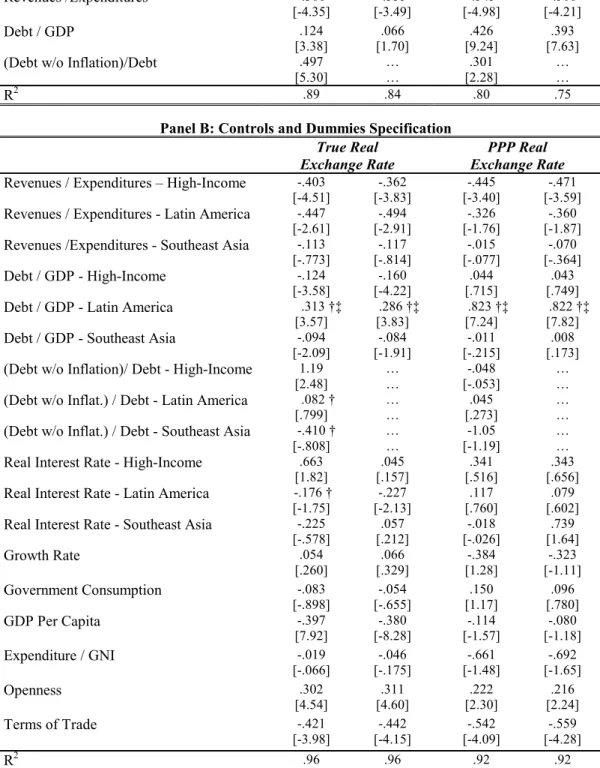
The estimated coefficients confirm the preliminary empirical evidence of section 2.3 and the model predictions from sections 2.4 and 2.5, where government budget deficits are associated with real exchange rate devaluations and lower stock prices. In general, the true real exchange rate definition gives a better fit (R2) and higher t-values than the PPP definition. The government
budget surplus elasticity, here specified in terms of governmentRevenues/Expenditures, is sta-tistically significant and negative, for high-income economies and Latin Americam middle-income economiesand also does not differ significantly across these economies.
The computed elasticities allow us to generate some quantitative estimations. Government ex-penditures averages for high-income and Latin American middle-income economies are respectively 30% and 21% of GDP and the elasticities estimated averages are δhiRE ∼=−.44 and δlaRE ∼=−.42. Thus, an increase of the surplus of 1% of the GDP will induce an approximate appreciation of the real exchange rate of (1/.3).(−.44) = 1.5%for high-income economies and (1/.21).(−.42) = 2% for Latin American middle-income economies.
Looking at the other fiscal variables we observe that Debt/GDP has a strong and positive impact on Latin America economies. One of the possible reasons is that government debt in foreign currency accounts for around 50% of total debt of these countries. For high-income and Asian economies the Debt/GDP elasticity tends to be negative and significant, but only for the true real exchange rate definition. One of the possible reasons is that for these economies, we could expect real interest rates close to or even lower than the growth rate of the economy; thus, keeping a constantDebt/GDP ratio indicates positive revenues for these countries.
2 7 For the robust regression estimators, White routine, robust estimates of the standard errors are
obtained from the variance matrix: (X0X)−1X0(P
i
P
jxij ij ijxij)X(X0X)−1where ij are the regression
residuals.
The Prais-Winsten regressions estimates assume that the error component follows a country specific AR(1) process:εit=ρiεi,t−1+ηit w/ηit∼N(0, σ2)and regress
yit−ρiyi,t−1=c(1−ρi)+a(xit−ρixi,t−1)+ηitfort >1and fort= 1
q
1−ρ2
iyi1=c
q
1−ρ2
i+a
q
1−ρ2
ixi1+
q
1−ρ2
iηi1.The last equation is the only difference between Prais-Winsten estimation and the
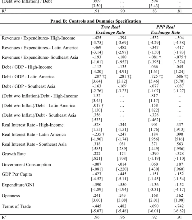
The last fiscal variable, (Debt without Inflation)/Debt, which measures revenues from part of the debt being inflated away, seems to be a relevant factor only for high-income economies for the true real exchange rate definition. This result could suggest that middle income economies, which present higher inflation rates, are not able to inflate away part of their debt, perhaps because of strong debt indexation.
The controls elasticities and semi-elasticities coefficients also present interesting results. For the GDP Per Capita, the negative and significant estimated elasticity is consistent with the Balassa-Samuelson effect, see footnote 10. The Expenditure/GNI coefficient confirms the Salter Effect: an excess of internal absorption relative to internal production is expected to appreciate the real exchange rate driving the excess of demand toward traded goods. The estimated coefficients also predict that more Openness and a fall on Terms of Trade are highly significant and tend to be positively correlated with real exchange rate devaluations.
Real Interest Rate, Growth Rate, and Government Consumption elasticities tend not to be statistically significantly different from zero at a 10% level. The exception is Real Interest Rate elasticities with respect to thetrue real exchange rate for Latin America economies, negative, and high-income economies, positive.
The inclusion of the variableDIit =ln(Debt without Inflation / Debt)measures the impact of inflationary revenues on debt. An alternative way to measure this impact is to use a different definition ofGovernment Revenues / Expenditures,one that takes into account the devaluation of government debt due to inflation as a source of government revenues. This alternative definition ofGovernment Revenues/ Expenditures starts from the fact that
Gov. Rev. Gov. Exp. =
Gov. Exp.-(Gov. Rev.-Gov. Exp.) Gov. Exp. = 1−
∆Real Debt Gov. Exp.
If we define the real value of debt fort≥1as
RDt=
Dt−1+(Expenditures−Revenues)t
Pt
t,and the real value of debt at t= 0 is defined as RD0 = DP00.Then, a definition of the ratio of
Government revenues to expenditures that takes into account the devaluation of the government debt due to inflation is given by
Gov. Rev. Gov. Exp.
0
= 1−RDt−RDt−1
Gov. Exp. (3.2.3) Although this definition takes into account inflationary revenues as a source of Government revenues, it does not present satisfactory results. Panel regressions using (3.2.3) as the definition of Government Revenues/Expenditures, which are not presented here, implied no statistically significant coefficients at a 5% level and lower R2 values for almost all regression specifications. The exception was the dummy for high income economies, which was negative and significantly different from zero at a 1% level.
3.3
Stock Price Regressions
The asset price formulas demonstrated in section 2 showed that government deficit has direct implications for stock prices. The intuition for this result relies on the fact that higher government deficits are in general persistent and a higher deficit today induces expectations of higher taxes and or higher inflation in the future, which decreases the discountedflow of expected future dividends. 28 Preliminary empirical evidence, which was discussed on section 2.3, also corroborates this observation.
This section intends to present even stronger evidence that stock prices are negatively cor-related with higher government deficits. For this purpose I used two regression specifications, a benchmarkBasic Specification and a more completeControls and Dummies Specification.29 The Basic Specification runs the regression
qxit=α+ϕRE(R/E)it+ϕDDit+ϕIDIit+ϕππit+ui+εit (3.3.1)
2 8Lower dividends due to high taxes are evident if dividends are taxed. The loss due to higher inflation,
however, relies on the assumption that dividends revenues have to be carried in cash from one period to the other.
2 9The sample excludes Uruguay, which has data for stock prices for the Total Market price index from
where the subscriptidenotes the country andtdenotes the time period,qx
it=log of the stock price index (xdenotes the numeraire used,National Currency orUS dollar),and as before(R/E) =log of government Revenues/Expenditures, Dit =log of total government Debt / GDP, and DIit = log of the variableDebt without Inflation / Debt andπit=inflation rate at time t obtained form the CPI index. Alternatively, I also run specification (3.3.1) without the variable DIit, since it tends to be highly correlated with the inflation rate.
TheControl and Dummies Specification, assumes that slopes for(R/E)it, Dit, πit,andDIit, for the group of high-income and middle income countries. Controls are used for Growth Rate, GDP Per Capita and totalGDP.
rerxit = α+ P g=hi,md
[ϕgRE(R/E)git+ϕgDDitg +ϕgDIDIitg+ϕgππgit]
+Ψ·(controlsit) +ui+εit (3.3.2)
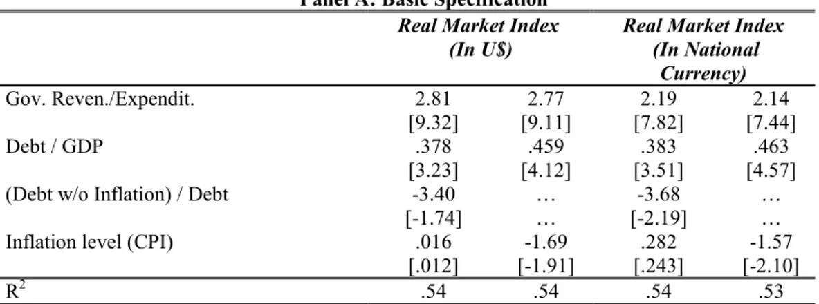
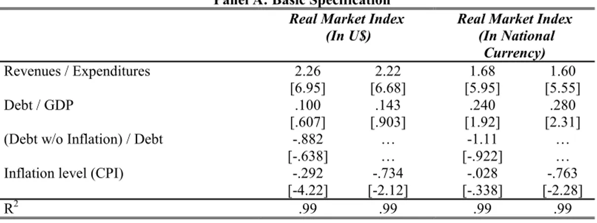
Table 4 presents the regression results forOLS estimates using the White routine while Table 5 presents Prais-Winsten regressions estimates. The results present strong evidence that higher deficits associated with lower stock prices. The average implied elasticity for ϕhi
RE ∼= .84 and
ϕmdRE ∼= 2.14 implies that an increase of 1% of GDP in the government budget deficit would be associated with a fall in stock prices in national currency on the order of 2.8% for the high-income economies and of 10.2% for middle-income economies.30 As opposed to the real exchange rates elasticities case, the government deficit has a quantitatively different impact on stock prices among industrialized and emerging economies.
For the Control and Dummies Specification, the impact of government debt to GDP ratio is statistically different from zero at a 1% level for the two groups of economies. However, while an increase in debt for high-income economies is associated with higher stock prices, the opposite is true for middle-income economies.
3 0For the high-income economies, government revenues average 30% of GDP, so the impact is computed
by(1/.3)ϕhi
RE. For middle-income economies, average revenues are 21% of GDP, which implies an elasticity
surplus to stock prices of(1/.21)ϕmd
RE.For the valuesϕhiRE andϕmdRE,I used the average of the coefficients
The impact of the inflation rate, ϕπ,is statistically significant at reasonable confidence inter-vals and negative only when the variable (Debt w/o inflation)/ Inflation, which measures debt devaluation due to inflation, is not included. This is a natural result, since (Debt w/o Inflation)
/Debt) ≡(Debtt+πtDebtt−1)/Debtt∼= 1 +πt, for small variations on nominal debt.
3.4
Country-Speci
fi
c Regressions
An alternative to the panel data regressions of Tables 2-5 would be to run a specific regression for each country. However, although this would allow less restricted estimates of countries ’ exchange rate and stock prices sensibilities, this choice would involve a sensible loss of observations in each regression specification. Since the panel-data used was unbalanced with at most 25 observations for each country, specific regressions would involve a much lower number of observations.
In order to verify the goodness offit of the pooled data regressions of sections 3.2 and 3.3 for specific countries, I computed R2 values for each country when the coefficients are restricted to
be the estimated panel data coefficients. The estimated countryi specificR20
i s are computed by the formula
R2i = 1−
Pni
t=1(eit−e¯i)2
Pni
t=1(yit−y¯i)2
(3.4.1)
where ni=the number of observations for countryi,yit=the value of the independent variable for country i,y¯i =sample mean for countryi independent variable,eit =regression residual for country i at time period t, ¯ei = sample mean for country’s i regression residual. Notice that although R2
i ≤1, we cannot guarantee that they are positive. ComputedR2
i for theOLS real exchange regressions with robust standard errors (Table 2) are presented on table 6, while the values for the OLS stock price regressions with robust standard errors (Table 4) are presented in Table 7.
Table 6 shows that the R2