Geostatistical Analysis: Software Flashpoint
J. Negreiros
1, M. Painho
2, A. C. Costa
3, J. Santos
4, I. Lopes
51
ISEGI - Universidade Nova de Lisboa, Campus Campolide, 1070-312, Lisboa, Portugal
Telephone: (351) 213870413Fax: (351) 213872140 Email: [email protected]
2 ISEGI - Universidade Nova de Lisboa, Campus Campolide, 1070-312, Lisboa, Portugal
Telephone: (351) 213870413 Fax: (351) 213872140 Email: [email protected]
3
ISEGI - Universidade Nova de Lisboa, Campus Campolide, 1070-312, Lisboa, Portugal
Telephone: (351) 213870413Fax: (351) 213872140 Email: [email protected]
4
ISEGI - Universidade Nova de Lisboa, Campus Campolide, 1070-312, Lisboa, Portugal
Telephone: (351) 213870413Fax: (351) 213872140 Email: [email protected]
5
Inst. Sup. Gestão - Inst. Politécnico de Santarém, Complexo Andaluz, 2001-904, Santarém, Portugal
Telephone: (351) 213870413 Fax: (351) 213872140 Email: [email protected] Abstract: Most spatial analysis computer programs are available on the ‘World Wide Wait’ leading this framework to a new GIS platform. Ultimately, this world expects fast answers because if it works then it is obsolete. To review and to evaluate the present spatial geostatistical analysis software and withdraw major conclusions regarding its implementation status are the major goal of this article. Among others, Surface® III, VarioWin®, Regard®, GSLib®, SpaceStat® and ESRI Geostatistical Analyst®are analyzed. Major conclusions regarding the present status of geostatistical software are drawn. Keywords: Geographical Information Systems; Spatial Statistical Analysis; Geostatistical Software; Geocomputation.
1. Introduction
The problem of statistical spatial analysis encompasses an expanding range of methods which address different spatial problems, from image enhancement and pattern recognition to spatial interpolation and socio-economic trend modelling. Each of these methods focuses on a particular aspect but what emerges is something that is clearly identifiable as spatial statistics, geographical raw data correlated by statistical methods.
Bação [1997], Anselin [1998] and Longley et al. [2001] argue that within specialized software there is a lack of spatial analysis techniques in general and of spatial statistics in particular. This may be a major impediment to GIS, which is a ‘data rich, theory poor’ environment. These authors put an emphasis on creativity, comparing spatial analysis to art and not to science. Applied geostatistics is a talent science because its results may be widely diverse depending on several factors such as the variogram modelling, the Kriging approach, the sampling design or the scientist’s previous experience.
There has been little progress in incorporating advanced spatial techniques into commercial GIS products in comparison to simple analytical functions. “Most of the functionalities should be more properly regarded as data manipulation rather than analysis” [Openshaw, 1998]. These functions are quite deterministic and include routing, site location, data summarization or vector-raster conversion. Certainly, future GIS issues should be viewed as questions of probabilistic thinking, e.g. the Modifiable Areal Unit Problem and Monte Carlo error propagation during an overlay operation. Moreover, dozens of research articles are printed every year with new spatial analysis methods, involving ever more fields such as stochastic simulation, multivariate geostatistic and spatial correlation. Regrettably, the majority of those ideas end up on the bookshelf without any practical consequence for the spatial analysis user. Algorithms, physical realities and thoughts exist for every person. A theory only succeeds if it leads to a practical purpose. “The spirit of geocomputation is fundamentally about matching the philosophy of science with practice, geometry with application, analysis with local context and technology with environment” [Longley et al., 1998]. To materialize research findings to the real world is a major dilemma nowadays since some of these methods are relatively crude because they have theoretical and implementation problems that remain to be solved. To review and to evaluate the present spatial geostatistical analysis software and withdraw major conclusions regarding its implementation status are the major goal of this article.
2. Geostatistical analysis software 2.1 Surface III®
Developed by the Kansas Geological Survey at the University of Kansas (http://www.kgs.ku.edu, retrieved March 2007), this software (797KB) is available for Macintosh® III+ version. Its input is a text file containing the coordinates and data
values. If a particular data location has multiple values then those values can be averaged or deleted. Contour lines and data postings can also be overlaid on shade maps but with the possibility of adjusting labels so that overprinting is minimized (Figure 1).
Figura 1 – The Surface III® data postings.
Surface III® produces spatial statistics including a map of the distance to the nearest,
farthest and average neighbours, the standard deviation for the distance and the number of the vicinity observations for a particular point and the number of octants and quadrants and the relative contributions of the nearest, farthest and average neighbours to the final estimate. Regarding griding algorithms, numerical arrays from uneven space data and square patterns are possible. Naturally, if a large grid cell size is chosen then the resulting map presents a low resolution and a coarse appearance but it can be computed quickly. In contrast, if grid cells are small then contour maps have a finer appearance with time consuming expenses. Transects and moving
averaging griding are further possibilities. Figure 2 introduces quadrant and octant searches, two methods that provide a search procedure for finding data points within a particular radius of the estimation point.
Figure 2 – The Surface III® search neighbourhood. 2.2 GSLib®
GSLiB®, an acronym for Geostatistical Software Library®, is a complete collection of
geostatistical programs developed by the Stanford faculty (http://www.gslib.com, retrieved March 2007) over the last 15 years, with two major goals: 1) to provide free geostatistical and simulation software to the public domain including Fortran® 77/90
source code; 2) to supply WinGSLib®, a commercial version for Windows (US $250).
Several aspects can be enhanced:
• Utilities programs (cell declustering, Normal Score Transformation, bivariate normal distribution for DK).
• Relative, general and pairwise variograms, madogram and Indicator variogram. • SK, OK, UK with nine monomials, IK, CK and SK with external drift.
• Stochastic simulation (Gaussian, Sequential, Indicator, Boolean, probability field, ellipsoid and simulated annealing).
• PostScript plotting utilities (normal QQ and PP plots, gray/color scale maps, Normal and lognormal probability plots).
Detailed information is provided by Deutsch and Journel [1997].
2.3 VarioWin®
This geostatistical shareware was created in 1995 by Pannatier at the University of Lausanne (http://www-sst.unil.ch, retrieved March 2007), Switzerland. Written in Borland C++®, this application is divided into four modules [Pannatier, 1996]:
Prevar2D, Vario2D, Model and Grid Display. The ability to handle datasets with UTM coordinates and the capability to read data files with empty lines are two attractive features of Prevar2D whose major goal is to build a distance matrix between all possible data pairs of the .DAT archive, and store it in a .PCF file. The Vario2D module uses the .PCF file to explore 2D experimental variograms. Another extended feature is to set limits for the active subset in relation to the x-axis, y-axis and other variables. The default estimator is the traditional variogram although the madogram, the correlogram and the covariance can be plotted too. The Model unit includes interactive geometric and zonal modelling with a particular characteristic: the Indicative Goodness-of-fit checks different nested models without forgetting the best fit model. The chosen model is also saved in an ASCII file but it includes the capability to produce a variogram model that can be copied into Gslib®.
2.4 REGARD®
Developed in 1990 in Pascal® at Trinity College Dublin for Apple Macintosh®,Regard®
seems to be distinguished Kriging software that allows simultaneous hot-linked interaction between data layers and views, including satellite imagery maps. This dynamic graphic capability is extremely useful for examining local variability and anomalies. Quoting Haslett et al. [1992], “we conclude that the most important single data view is the Map View: all others must be cross-referred to this one and future applications must encourage this concept”. It includes overlay plots on the background and brushing with many update links maps. The Map View and the Histogram View help the user to visualize potentially significant spatial patterns. “The recognition of spatial discontinuities and other anomalous behaviour makes one reluctant to rely overly on any interpolation procedures at an initial stage for most data” [Haslett et al., 1992]. According to Gunnink and Burrough [1996] and regarding the 100 zinc concentration measurements at the river Meuse, Netherlands, the highest histogram selection lies along the river borders (Figure 3).
Figure 3 – The Regard® brushing and linking features.
The Map View also provides a mechanism for the user to define a window and to drag it, under mouse control, over an appropriate region. As it passes over data points, statistics are produced, like the constant updated mean or variance in the Trace View window. Hence, the direct control of spatial analysis and encouragement to experiment is stressed. It is possible to select data points on the variogram cloud and highlight them on the Map View. Also, the Scatterplot Matrix View among variables can suggest the possible existence of two populations (Figure 4).
Figure 4 – The Regard® brushing and linking features within the scatterplot view.
The Rescaled Variogram Cloud View uses the robust estimator proposed by Cressie and Hawkins (1980). The pairs selection of the Map View rescaled cloud that are closed in space but different in values are another attractive feature because these are the ones that most contribute to the nugget-effect. If these pairs are well scattered in space
then outliers can be found. If these samples are concentrated in a particular region then local pockets of non-stationary emerge.
2.5 ArcGIS Geostatistical Analyst® Module
This ESRI® extension (http://www.esri.com/software/arcgis/extensions/geostatistical,
retrieved March 2007) involves variogram modelling which includes graphical and automatic anisotropy assessment, covariance surface layout and neighbourhood search size to a limited number of points used in prediction. Its wizard includes four major steps, thus allowing new users to produce an easy surface with the default parameters:
1) Input and methodology;
2) Variance/covariance modelling; 3) Search neighbourhood;
4) Cross-validation and validation with a new test dataset.
As with other geosoftware, it offers histograms and a normal QQ plot for a Gaussian distribution check, OK, UK and DK, trend analysis in a 3D environment for global trend detection and Voronoi as a spatial variability assessment. This includes the nugget-effect division into microstructure and measurement error. Concerning the cross-validation procedure, four statistics are presented: the mean prediction errors, the root mean square, the average standard error and the root mean square standardization. Cross cross-validation based on an alternative new sampling dataset is an option. The prediction standard error surface for each location can be plotted. In conjunction with other boundaries layers such as hill shade, grid, transparency and filled contours, IK and PK for threshold probability mapping are also feasible. Finally, probability, quantile and prediction standard error maps can be computed from SK, OK, DK, UK and CK. Regarding deterministic approaches, five Spline functions, IDW, and ten global (fitting a polynomial to the entire surface) and local (fitting many polynomials, each within specified overlapping neighbourhoods) polynomial orders are covered. According to ESRI [2001], “IDW optimal power is determined by the minimized root mean square prediction error in a cross-validation framework”. In other words, Geostatistical Analyst® tries different powers and, according to the resulting root mean square
prediction error, the power that provides the smallest one is the optimal exponential. Another single feature of ESRI® GIS extension is the Normal Score Transformation
dialog box, a ranked-based method including direct (using the observed cumulative distribution), linear (fitting lines between each step of the cumulative distribution) and Gaussian (based on a smoother probability density function) approximation resolution. In addition, the conventional declustering methodologies of cell and Voronoi polygons can be used. Some other major features are offered:
•
Similar to Regard®, the brushing operation is applied intensively between theArcMap® and the corresponding selected points in the histogram, normal QQ plot,
variance cloud, Voronoi map and two dataset cross-covariance cloud views. • The capability of computing measurement error, if the user possesses multiple
measurements per location, makes this module unique too. • Data classification is viable through the creation of range classes.
•
The search neighbourhood includes directional influences, the maximum and minimum number of locations to use and the sectors division number.•
The following variogram functions are provided: circular, spherical, tetraspherical, pentaspherical, exponential, Gaussian, rational quadratic, wave-hole, K-Bessel, J-Bessel and stable.2.6 SpaceStat®
SpaceStat®, a self-contained Windows® 2000 and Millennium® software package
written in GAUSS® for lattice data (http://www.terraseer.com/products/spacestat.html,
retrieved March 2007), is organized into four modules. The data module allows merging files, to recode variables and to create dummy categorical indicator variables for a given range. Note that the input files (contiguity, spatial weight and auxiliary) must be converted into GAUSS® binary format for a post-processing operation. This includes
principal component analysis.
The spatial tools module for spatial weight manipulation consists of:
•
Creation of the W matrix based on the Euclidean and great circle distance with standardization and the capability of dissolving areas units;•
A characteristic report for the W matrix; • Information on the connectivity structure;• Construction of the contiguity weights using the rook/bishop/queen criterion (the Raster Wts option);
•
The W eigenvalues and the trace index calculation [Anselin, 1992].If the contiguity matrix only contains {0,1} information then SpaceStat® follows the
GAL format (FMT files). Thus, the corresponding ASCII input file contains the number of observations and, for each observation, it lists its identifier, the number of contiguous observations and their respective identifiers. Regarding the weights of the sparse format, this input file contains the number of observations and, for each non-zero weight element, it lists the identifier for the row and column followed by the weighted value. Remark that the GAUSS® matrix format is unreadable by standard editors or
word processors. The symmetry lacking due to the typographical errors can be checked. The contiguity structure between observations can also be recorded visually by inspecting a map or by running an AML® macro within ArcInfo®. Another possibility
is to define the lower and upper bounds for a distance band definition.
The Explore unit for spatial association measures presents a diversity of spatial autocorrelation measures such as the Moran scatterplot, Moran I, the spatial correlogram, Gary C, global G(d) and local Gi by showing the ten highest and lowest
values. The join-count statistics for spatial autocorrelation as an ESDA tool is also undertaken with the Data-Var Create-Create Dummy Variables option.
The generic OLS and robust OLS regression for non-homoskedasticity situations are computed within the spatial regress module. As expected, the R2 and adjusted R2
indices, the t-Student for regression coefficients and the global F test are also reported. Although both OLS techniques lead to the same coefficients and prediction values, their variances are quite different if spatial autocorrelation among errors or heteroskadasticity exists. An alternative method to overcome heteroskedasticity is based on the Regress Heterosked Error option, a GLS procedure.
2.7 GMS®
GMS® is a comprehensive ten-module package that provides tools for groundwater
simulation including site characterization, model development, post-processing, calibration and visualization (http://www.emrl.byu.edu/gms.htm, retrieved March 2007).
It also supports TINs, 2D and 3D geostatistics and other groundwater simulation techniques. Some other attributes are offered:
• Any dataset simulation can be converted to an animation film loop saved in AVI format.
• Clough-Tocher interpolation, the moving weighted average and mapping elevations are incorporated.
• Data Calculator allows the comparison of two interpolation dataset fields.
•
IDW, OK, UK, IK and Indicator simulations are covered by GMS®.•
Imports/exports includes raster and vector GIS data from/to ArcInfo®, ArcView®,GRASS® and DXF® files for AutoCAD®.
•
The PC version runs on Windows® 2000 while the Unix® version is available forCompaq® Alpha, HP® Unix®, SGI® Irix and Solaris® platforms.
• Images can be copied to the clipboard and pasted into other applications for report generation.
•
The Mt3dms module is particularly suited for migration
simulation of contaminant plumes over time.
2.8 KRIGING for Berkley UNIX®
The goal of this project
(
http://www.nbb.cornell.edu/neurobio/land/OldStudentProjects/cs490-94to95/clang/kriging.html, retrieved March 2007), created by Lang [1997] at the Computer Science Department of Cornell University, was to implement an OK module using spherical and exponential variograms for Unix® IBM RS/6000 and HP-700®, a
system V of the Berkley® Software Distribution version [Negreiros et al., 1998]. An
useful feature is illustrated in Figure 5: the left image illustrates the estimated layout while the right one uses a colour map to display error variance. Since the location of the white dots represents input samples, it becomes clear that the error variance is smaller in the presence of abundant observed data.
Figure 5 – The Kriging for Berkley Unix® Ordinary Kriging interpolation and variance. 2.9 ECOSSE®
Developed by Alloa® Business Center (http://ecossenorthamerica.com, retrieved March
2007), this remarkable geostatistical software was written in Visual Fortran® 90 for
Windows®. If sample distribution follows the ‘bell’ curve, EcoSSe® presents the
‘grade/tonnage’ curve whose cutoff probability plot is introduced and based on the estimated mean, standard deviation and probability population above the cutoff limit. Based on Sichel´s correction factor, the lognormal transformation is also covered, including the plotting of the cumulative density function and other descriptive statistics. In addition, the linear regression relationship based on logarithms and ranked transform in accordance with nonparametric statistical analysis is possible.
The linear, quadratic and cubic polynomial trends can be used within EcoSSe® as a
global estimator or as a detrend Kriging process. Particularly, it is the random residuals variogram that confirms the detrend polynomial decision. If the remaining residuals show rises, peaks and falls, then an over-fitting data surface is made and, hence, a lower polynomial model is needed. “The variance in residuals and the corresponding variogram sill should also be identical suggesting that the variogram will be a good variation indicator” [Clark and Harper, 2000]. Another two single features highlighted by EcoSSe® are:
• The nearest neighbour option gives the average and the closest distance among samples.
•
The geographical area definition specifies the area through a file that contains the boundary information about the field for sampling limitation purposes.2.10 GEOPACK ®
GeoPack® is a DOS package for conducting analyses of spatial variability with up to ten
variables (http://www.epa.gov/ada/csmos/models/geoeas.html,
retrieved March
2007). The basic statistics includes mean, median, variance, standard deviation, skewness, kurtosis, maximum/minimum and coefficient of variation. It also includes linear and polynomial regression, the Kolomogorov-Smirnov test for Normal distribution and percentiles calculation. According to Ella [2000], “the variogram models can be fitted using the fitting procedure of nonlinear least-squares developed by Marquardt or the traditional manual interactive approach”. GeoPack® embraces OK and CK alongwith their associated estimation variance and conditional probability for a specific cutoff level. IK, OK and BK with geometric anisotropy are also integrated. Nonlinear estimators such as the parametric DK and disjunctive CK can also be assessed with the estimation variance. Up to ten cutoff levels are allowed.
2.11 UNCERT®
According to Wingle et al. [1999], Uncert® is 2D and 3D geostatistical software applied
to groundwater flow and contaminant transport modelling for Unix® workstations that
run X-Windows and Motif®. Besides the traditional GUI, it also works from the command
line or in batch mode, which is particularly useful for large datasets or to process the Monte Carlo simulation (http://uncert.mines.edu/software.shtml, retrieved March 2007). This software is organized into several modules:
• Plotgraph is an X-Y graphic tool that performs least-squares regression for up to tenth order polynomials.
• Histo displays univariate statistical data and, with up to 20 populations, it can be compared simultaneously.
• Distcomp allows different data populations to be displayed together using histograms and general QQ plots.
• Vario calculates experimental variograms and other spatial relations such as covariance, correlograms, log variograms, madograms, indicator variograms and cross-variograms.
• Variofit fits the experimental variogram using least squares regression techniques and the jackknife techniques. Spherical, exponential and Gaussian models with up to four nested structures plus nugget-effect are also included. • Contour provides a 2D contouring utility for regular grids including posted labels,
direction arrows and line work representing roads, buildings or formation contacts, for instance.
•
Block is a utility for viewing 3D scattered and grid data.•
Modmain and mt3dmain offers a complete GUI interface for MODFLOW® andMT3D® simulation models with animation.
•
Array is a tool for mathematical calculations on grid data like variance estimation or cell frequency for a specific range. Constants can be added, subtracted, multiplied or divided for every cell. In addition, cells can be reclassified on the basis of their value.• Grid module is responsible for interpolating data using three methods: IDW (residuals are evaluated at each sample location), trend surface analysis (up to fifth order) and Kriging (SK, OK and UK) including the cross-validation procedure. Kriged residuals from trend surface analysis are also possible to compute.
3. Conclusions
“…Promote the diffusion of analysis based on GIS throughout the scientific community and provide a conduit for disseminating information regarding GIS research, teaching and applications.”
NGCIA, 1996, Annual Report
Clearly, two methods emerge regarding spatial interpolation: the deterministic and the stochastic view. If the former has no capability for assessing uncertainty, the latter must be viewed as a process instead of a single function with an increase in computer power demand, particularly with Kriging. In terms of software development, highly regarded literature such as Longley et al. [1998] refers to three major implementations: independent geosoftware, GIS modules and statistical packages with spatial extensions. Data exchange among systems has also become a requirement. In fact, spatial analysis and GIS are well-established technologies that operate in different spheres at present although their aims are similar: to describe and to infer the nature of spatial variation. Hence, some kind of systems integration would benefit both groups of users: within GIS, by increasing the scope of their spatial analysis and, within spatial analysis, by providing topology access. Yet, the lack of spatial autocorrelation measures in the software is huge. In fact, these measures may also help the variogram fitness interactive procedure. To date, the WWW implementation environment has never been considered.
Among most software, Geostatistical Analyst is revolutionary because it fills the gap between geostatistics and GIS since geostatistical software has never been completely integrated within GIS by the same corporation. In combination with ESRI® ArcCatalog®
for metadata purposes, layers operations can also be accomplished such as zooming, panning, layer name changing, copying, removing, and exporting geostatistical layers to raster or vector formats.
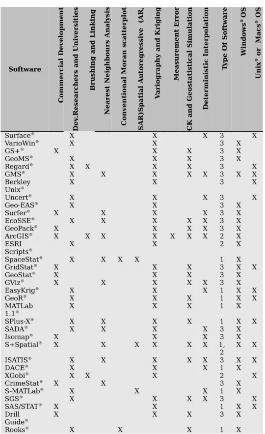
Table 1 shows other software packages reviewed (though not discussed here in detail) by presenting their main features summary. This includes GridStat®, GeoStat®, GViz®,
EasyKrig®, GeoR®, MATlab 1.1®, SPlus-X®, SADA®, Isomap®, S+Spatial®, ISATIS®,
Software C omm ercia l De velopme nt Resea rchers and Un ive rsi ties Dev . Br ushing and Lin king Nea rest Neighbo urs Analysis C on ventio nal M or an s catterplot Spatial Au tor egressive (AR, SA R) V ariograp hy and Krigi ng Measur eme nt Error CK and Geos tatistical Simulatio n Determi nistic Interpol ation T ype Of Softwar e W indows ® OS Unix ® or Macs ® OS Surface® X X X 3 X VarioWin® X X 3 X GS+® X X X 3 X GeoMS® X X X 3 X Regard® X X X X 3 X GMS® X X X X X 3 X X Berkley Unix® X X 3 X Uncert® X X X 3 X Geo-EAS® X X 3 X Surfer® X X X X 3 X EcoSSE® X X X X X 3 X GeoPack® X X X X 3 X ArcGIS® X X X X X X X 2 X ESRI Scripts® X X 2 X SpaceStat® X X X X 1 X GridStat® X X X 3 X X GeoStat® X X X 3 X GViz® X X X X X 3 X EasyKrig® X X X 1 X X GeoR® X X X 1 X X MATLab 1.1® X X X 1 X SPlus-X® X X X X 1 X X SADA® X X X X 3 X Isomap® X X X 3 X S+Spatial® X X X X X X 1, 2 X X ISATIS® X X X X X 3 X X DACE® X X X 1 X XGobi® X X X 2 X CrimeStat® X X 3 X S-MATLab® X X X 1 X SGS® X X X X 3 X SAS/STAT® X X 1 X X Drill Guide® X X X 3 X Rooks® X X X 1 X
Table 1 – Analysis of geostatistical software (1 – Statistical Package; 2 - GIS Module; 3 - Independent Geosoftware).
According to the previous sections and Table 1, some major inferences can be drawn:
•
Commercial costs arise with some of geostatistical software, like the ESRI®•
Non-commercial software offers its computer code (which varies from C++® toPascal®, Fortran®, C®, Excel® macros, statistical scripts, Gauss® and VBasic®), a
trend that is not followed by a few non-commercial options;
• No software establishes a close link between Kriging and the Moran scatterplot;
•
No statistical packages that cover spatial autocorrelation issues such as Rooks®or Spacestat® handle simple observations with no defined boundaries;
•
Only SpaceStat® and S+Spatial® deal with spatial autoregression andautocorrelation issues;
•
All Kriging packages compute the OK variance, cross-validation procedure and classical statistics indices while the K-density and variable transformation functions are only available in a few ones such as SPlus-X®, CrimeStat® or GS+®;•
Measurement error is only considered by the ESRI® Geostatistical module;• No software presents an e-Learning framework for educational purposes;
•
Interfaces range from a window and batch mode to command lines. The Web interface in a Web application framework was never considered;•
Only three software, Regard®, ArcGIS® and XGobi®, allow the brush and directmap linkage features;
•
Most software pursues the black-box strategy, like Variowin® for example, whileothers demand a complete understanding of geostatistics background files, like GSlib®;
• All software has a specific installation procedure, depending on the operating system;
•
Most software has a specific input format although interoperability, particularly with ASCII files, can be achieved.References
Anselin, L., SpaceStat Tutorial - A Workbook for using SpaceStat in the Analysis of Spatial Data, University of Illinois, Urbana-Champaign, 1992.
Anselin, L., Exploratory spatial data analysis in a geocomputational environment. In: Paul Longley, Sue Brooks, Bill Macmillan and Rachel McDonnell (eds.), GeoComputation, a Primer. New York: Wiley, 1998: 77–94.
Bação, F., Os Sistemas de Informação Geográficos e as Empresas, Dissertação de Mestrado em Estatística e Gestão de Informação, Instituto Superior de Estatística e Gestão de Informação, Univ. Nova de Lisboa, 1997.
Clark, I., Harper, W., Practical Geostatistics 2000, Ecosse North America, Columbus, Ohio, USA 2000.
Cressie, N., Hawkins, D.M., Robust estimation of the variogram: I. Mathematical Geology, 12(2), 1980: 115-125.
Deutsch, C., Journel, A., GSLIB: Geostatistical Software Library and User's Guide, Oxford University Press, 1997.
Ella, V., Spatial Analysis And Simulation Of Selected Hydrogeologic And Groundwater Quality Parameters In A Glacial Till Acquitter, Ph.D. Thesis, Iowa State University, 2000. ESRI, Using ArcGIS Geostatistical Analyst, USA, 2001.
Gunnink, J.L., Burrough, P.A., Interactive spatial analysis of soil attribute patterns using Exploratory Data Analysis (EDA) and GIS. In: M. Fischer, H.J. Scholten and D. Unwin. (eds), Spatial analytical perspectives on GIS, Taylor & Francis, London, 1996: 87-100. Haslett, J., Bradley, R., Craig, P., Unwin, A., Wills, G., Dynamic Graphics For Exploring Spatial Data With Application To Locating Global And Local Anomalies, The American Statisticien, Vol. 45, 3, 1992: 234-242.
Lang, C., Kriging Interpolation, http://www.cs.cornell.edu, 1997.
Longley, P., Brooks, S., Macmillan, B., McDonnell, R. (eds.), GeoComputation, a Primer. New York: Wiley, 1998.
Longley, P., Goodchild, M., Maguire, D., Rhind, D., Geographical Information Systems and Science, John Wiley & Sons, 2001.
Pannatier, Y., VARIOWIN: Software for Spatial Data Analysis in 2D, Springer-Verlag, New York, NY, 1996.
NGCIA, Annual Report. National Centre for Geographic Information and Analysis, Year 7 (January 1, 1995 - December 31, 1995), University of California (Santa Barbara), State University of New York at Buffalo, University of Maine, USA, 30 March 1996.
Negreiros, J., Amador, J., Castro, J., Unix-Curso Completo, FCA-Lidel, 1998.
Openshaw S, Building automated geographical analysis and explanation machines. In: Longley P, Brooks S, Macmillan B and McDonnell R (eds), GeoComputation, a Primer, Wiley, New York, 1998: 95-115.
Wingle, W.L., Poeter, E.P., McKenna, S.A., UNCERT: geostatistics, uncertainty analysis and visualization software applied to groundwater flow and contaminant transport modelling, Computers and Geosciences, 25, 4, 1999: 365-376.