Spatial statistical analysis and selection of genotypes in plant breeding

Spatial statistical analysis and selection of genotypes

in plant breeding

João Batista Duarte(1) _{and Roland Vencovsky}(2)

(1)_{Universidade Federal de Goiás, Escola de Agronomia e Engenharia de Alimentos, Caixa Postal 131, CEP 74001-970 Goiânia, GO, Brazil.} E-mail: jbduarte@agro.ufg.br (2)_{Universidade de São Paulo, Escola Superior de Agricultura “Luiz de Queiroz”, Dep. de Genética, Caixa Postal} 83, CEP 13418-070 Piracicaba, SP, Brazil.

Abstract – The objective of this study was to evaluate the efficiency of spatial statistical analysis in the selection of genotypes in a plant breeding program and, particularly, to demonstrate the benefits of the approach when experimental observations are not spatially independent. The basic material of this study was a yield trial of soybean lines, with five check varieties (of fixed effect) and 110 test lines (of random effects), in an augmented block design. The spatial analysis used a random field linear model (RFML), with a covariance function estimated from the residuals of the analysis considering independent errors. Results showed a residual autocorrelation of significant magnitude and extension (range), which allowed a better discrimination among genotypes (increase of the power of statistical tests, reduction in the standard errors of estimates and predictors, and a greater amplitude of predictor values) when the spatial analysis was applied. Furthermore, the spatial analysis led to a different ranking of the genetic materials, in comparison with the non-spatial analysis, and a selection less influenced by local variation effects was obtained.

Index terms: augmented design, mixed model, information recovery, autocorrelation, correlated data, geostatistics.

Seleção de genótipos e análise estatística espacial no melhoramento

de plantas

Resumo – O objetivo deste trabalho foi avaliar a eficiência da análise estatística espacial na seleção de genótipos de plantas num programa de melhoramento. Buscou-se demonstrar os benefícios potenciais dessa abordagem quando as observações experimentais não são espacialmente independentes. O material consistiu de um ensaio de competição de linhagens de soja, com cinco cultivares testemunhas (de efeitos fixos) e 110 novos genótipos (de efeitos aleatórios), delineado em blocos aumentados. O ajuste espacial foi feito pelo modelo linear de campo aleatório (RFLM), com função de autocovariância estimada a partir dos resíduos da análise sob erros indepen-dentes. Os resultados apontaram uma autocorrelação residual de magnitude e alcance significativos, o que garantiu à abordagem espacial uma melhoria considerável na discriminação dos tratamentos genéticos – aumen-to do poder dos testes estatísticos, redução nos erros padrão de estimativas e de prediaumen-tores e alargamenaumen-to na amplitude das predições genotípicas. A análise espacial levou a um diferente ordenamento das linhagens em relação à análise não espacial e, finalmente, a uma seleção menos influenciada por efeitos da variação local. Termos para indexação: delineamento aumentado, modelo misto, recuperação de informação, autocorrelação, dados correlacionados, geoestatística.

Introduction

In plant breeding, two features indicate the preliminary phases of selective programs: the large numbers of new genotypes to be evaluated and the small amount of ma-terial for their propagation. Both of them limit the use of replications of these genetic treatments, which are frequently evaluated in a single experimental plot, i.e., without replications. Federer (1956) proposed the augmented experimental designs to deal with this type

of limitation, which allow the adjustment of the test line (new treatment) means for environmental effects (blocks, lines, or columns) estimated on the basis of repeated check genotypes. The author also presented the corresponding methods of statistical analysis, based on ordinary least squares (OLS) and, therefore, on the assumption of independence among observations.

plants. This increases the chance of violating the independence among observations assumed when using the OLS method, due to the likely similarity of observations of neighboring plots (Stroup et al., 1994). This phenomenon, referred to as spatial correlation – also called spatial dependence or autocorrelation – can seriously affect the comparison of treatments. Es & Es (1993) have demonstrated that when this correlation occurs, the statistical tests associated with contrasting treatments in plots nearer together have higher probabilities of type II error, which consists of different treatments appearing to be identical. On the other hand, higher probabilities of type I error, i.e., identical treatments appearing to be different, were observed in the contrasts between treatments in which plots were farther apart.

The traditional analysis of variance relies on randomization to neutralize the harmful effects of this type of correlation, but frequently this is not attained adequately (Stroup et al., 1994). For this reason, Kempton et al. (1994) support a greater use of methods that consider some accounting for spatial dependence to improve the precision of variety trials. Recent advances in statistics for spatially distributed data have provided a number of alternative methods. One interesting approach is that of Zimmerman & Harville (1991). In this analysis, the plot effect (trend + error) is modeled in such a way that the observations are collectively taken as a partial outcome of a random field, similar to predictive models used in geostatistical applications (Martínez, 1994). The model aims at estimating the general covariance function, which is used in estimation and prediction, through generalized least squares (GLS). Therefore, it is a mixed linear model with spatially correlated errors, called a random field linear model (RFLM).

Due to the relatively limited use of these techniques among plant breeders, it is necessary to assess their effects on selection of genotypes to finally demonstrate their true potential. This study illustrates the application of the RFLM approach, adapting it to the augmented block design, which is typical in the preliminary phases of the selection process in plant breeding. The attempt does not intend to represent the best spatial approach for the set of data analyzed, but, rather, to demonstrate the benefits of a less restrictive statistical analysis in comparison with the traditional one, based on spatially independent observations.

Material and Methods

The data used in this study were obtained in a soybean variety trial, with F6:3 lines of the semi-early maturity group,

conducted in the locality of Areão, municipality of Piracicaba, SP, Brazil, in 1999/1995. The trial is part of a selection program conducted to increase soybean yield, carried out by the Department of Genetics of Esalq/USP. Genetic materials were evaluated in augmented block design, witht t = 5 check varieties (Bossier, Davis-1, IAC-12, IAS-5 and Viçoja) and p = 110 test lines, distributed in b = 4 blocks with approximately 50 plots each. The plot corresponded to two rows of plants, spaced 0.6 m apart and 5 m long. Only grain yield data (kg ha-1_{) were considered here. For}

spatial statistical analysis, it was necessary, in addition, to obtain the distances (meters) among plots, which was done from the geographical coordinates of the center of each plot in the experimental field grid – COORDX represents the width coordinate of the plots and COORDY, the length coordinate.

Two mathematical models were used for statistical analysis: i) a model which assumes spatially independent observations; and ii) a model allowing spatial correlations among observations. In both cases, the effects of test lines were taken as random, and here were assumed to be derived from a single base population, that is, varying randomly about a common mean. For this reason, the independent error analysis here does not correspond to the fixed model (OLS). Thus, both are mixed models, despite the adjustment for checks. The only difference between them is the assumption on the experimental error.

In the case of spatially independent observations, this analysis is described as intergenotypic information recovery analysis (Wolfinger et al., 1997; Federer, 1998). One peculiarity of such analysis in the augmented designs is that the mathematical model needs to accommodate two types of treatment effects: fixed effects for the checks (t populations) and random effects for the test lines. These lines constitute the (t+1)th _{population, which}

is also assumed to have a fixed effect. Thus, in the first alternative (i), the observations can be individually characterized by the model (an adaptation to the model of Scott & Milliken, 1993, proposed by Duarte, 2000): Yijk=µ + bj + ck + gi(k) + eijk

in which Yijk is theobservation in the plot with genotype i,

stemming from population k in block j; µ is the constant common to all observations; bj is the fixed effect of the

jth _{block (j=1,2,...,b); ck is the fixed effect of the k}th

the population of lines); gi(k) is the effect of the ith

genotype within the kth _{population, assumed to be fixed}

and with a null mean, if the genotype is a check (i(k) = 1),

or random with independent distribution N(0, 2 g

σ ), if the genotype is a test line (i(k)=1,2,...,pk , with Σpk = p); and

eijk is the random experimental error associated with

the ijkth _{plot, which is assumed to be independent, that}

is, null covariance among the errors of different plots, and with distribution N(0, 2

e

σ ).

In model (ii), the term eijk is assumed to have the

distribution eijk ~ N [0,C(h)], in which C(h) is the covariance

between two errors of plots which are h units of distance apart (h≥0). If such errors are denoted by e(s) and e(s+h), in

which s represents the spatial position of the ijkth _{plot, in}

the RFLM approach, C(h) is defined as (Littell et al., 1996):

C(h)=

   

σ = σ

σ

0 h> if , ] f(h) [

and ; 0 = h if ,

2 (s+h) e , (s) e 2

Thus, it is assumed that the covariance of the errors is a function of the distance that separates the corresponding plots (f(h)). However, this is not predetermined, but is estimated from the “uniformity experiment” suggested by the residuals (

eˆ

Representing the observations by a vector y, both models can be expressed in matrix notation by the ge-neral mixed linear model (Henderson, 1984): y = Xβ + Zγ + ε; with γ~N(φ,G), ε~N(φ,R), E(y)=Xβ and

Var(y) = V= ZGZ' + R.

The fixed effects are in parametric vector β; the random effects, in parametric vector γ, except the errors that are in vector ε; X and Z are incidence matrices of the effects contained in β and γ, respectively. The random genotypic effects (γ) are assumed, without loss of generality, to have a normal distribution with a null mean (φ) and matrix of covariance G = I 2

g

σ (where I is an identity matrix). The experimental errors are presumed to have a normal distribution with a null mean and a generic matrix of covariance R. Thus, in the first model (i), R = I 2

e

σ , while in the other (ii), R = Σ, i.e., a non-diagonal matrix with structure defined by the general covariance function and by the autocorrelation range.

The first step in this spatial analysis is the adjustment of the model which postulate spatial independence among observations. The components of variance σ2_g

and 2

e

σ were estimated by restricted maximum likelihood

(REML). The estimated residual vector of this adjustment is: εˆ=y−yˆ, with yˆ₌X_β0 ₊Z~_γ, in which

y V X ) X V X

( 1 1

0 _{= ′} − − _′ −

β and ~_γ=GZ_′V−1(y₋X_β0)_,

representing the solution vectors of the mixed model equations (Henderson, 1984). The residuals were then used to estimate the spatial correlation structure. This was done graphically by means of a so-called semivariogram or simply variogram (Stroup et al., 1994). In this graphic representation, estimated values of semivariance, (h)Sˆ , are plotted against their respective distances h, resulting in a scatter plot (sample variogram). The semivariance is defined as: S(h)=½Var[e(s+h) −e(s)];

which is estimated by = ∑ ₊ −

N(h)

2 (s) h) (s N(h)

2 1 [eˆ eˆ ]

(h)

Sˆ , with

N(h) being the number of differences at the distance h. In this graph, values (h)Sˆ that are distributed randomly as a function of h reflect independent observations (residuals). The typical configuration of spatial dependence among observations occurs if values (h)Sˆ tend to increase as h increases up to a certain distance (range), after which the semivariance stabilizes reaching a plateau (or sill). Less variability is associated with smaller distances. The spatial correlation range (a) is the mean distance influence of an observation (plot), asserted here to be uniform in all directions (isotropy). The sill (_σ2_{) corresponds to the intrinsic variance of the}

variable under study (Var[e(s)] = Cov[e(s),e(s)]), which is

also equivalent to the covariance between residuals of plots separated by a distance equal to or greater than the range (Cov[e(s),e(s+h)], with h≥a).

There is an advantage in evaluating spatial dependence by means of the variogram. Under stationarity – spatial law unaffected by translation – the variogram has a direct and simple relation to the function of autocovariance C(h), that is: S(h) = σ2_{-C(h); in which σ}2 _{= C(h = 0)}

software that facilitates this adjustment is available (ex: Variowin; Geo-Eas). In such programs, the search for the function that best fits the observational points is carried out by changing slightly the values of σ2 _{and a.}

In the present case, the exponential model provided the best fit, corresponding to the following covariance function (for isotropic random fields):

) ( exp C(h)_=σ2 _−a3h _.

After defining parameters (σ2 _{and a) and the}

gene-ral covariance function, the next step is fitting the model to account for spatial dependence (R = Σ). This involves obtaining estimates, predictors, and statistical tests related to treatment effects, which must be free from estimated autocorrelation effects. To evaluate only the effects of the spatial adjustment on the statistical analysis, the same estimate of σ2_g obtained in the former analysis (under

R = I 2

e

σ ) was used. The following procedure consisted of resolving the mixed model equations (Henderson, 1984):       Σ ′ Σ ′       γ β       + Σ ′ Σ ′ Σ ′ Σ ′ − − − − − − − y Z y X = ~ G Z Z X Z Z X X X 1 1 0 1 1 1 1 1 ,

which solutions have already been reported.

Results and Discussion

Characterization of spatial covariance

The experimental data showed a positive spatial correlation of first-order to sixth-order, in the series of residuals (Table 1). This fact is indicative of the violation of spatial independence among observations postulated by the first model (under R = Iσe2). Residuals of this

analysis were not randomly distributed in the experimental field (Figure 1). Rather, there is a clear tendency for larger residual values (eˆ ) to be concentrated in theijk

top of the field map graph, that is, to be associated with plots having smaller COORDX values.

This fact also determined a predominant gradient in the direction of plot widths (COORDX). Considering this is how the blocks were constructed, it is possible that such an orientation may not have been ideal. Given the features of the residual surface, which provides an estimate of the uniformity trial underlying the experiment, it is reasonable to suppose that a lengthwise blocking of the plots would have been more effective in controlling local variation. The possibility of making this diagnosis represents an advantage of the spatial approach, which creates perspectives for the application of alternative forms of a posteriori local control or post-blocking

(Federer, 1998).

The variogram obtained for distances less than 30 m is showed in Figure 2. The configuration of the dots is typical of stochastic processes with spatial dependence, that is, with decreasing variability as distance decreases. After 20 m (range) the variability tends to stabilize. The value of this plateau represents the residual variance among independent plots, and the existence of the increasing variogram with a plateau is an indication that the intrinsic hypothesis of stationarity was satisfied (Vieira, 2000). Furthermore, on the assumption of isotropy, the continuous function that best fits the dots is the exponential semivariance model:

)] ( exp 1 [

S(h)_=σ2 _{− −a}3h _{, with:}

σ2=126450 (kg ha-1)2

and a = 20.4 m. Consequently, the respective autocovariance function is expressed by

) ( exp 126450

C(h)_{= 6}−_.h_{8 . This defines the residual}

Table 1. First to tenth-order autocorrelations (ρˆ) and the

respective Durbin-Watson statistics (d) for the residual (eˆijk)

series obtained from the adjustment of an augmented block design model with independent errors.

(1)_{Marginal probability of the statistical test (H}

0:ρ=0) (one-sided to

the left, in this case).

Figure 1. Residuals (kg ha- 1) of the augmented block design

model adjustment, with recovery of test lines information, under independent errors as a function of the plot center coordinates, in meters (COORDX and COORDY).

Order

ρ

ˆ

covariance matrix R = S, whose main diagonal elements were all equal to 126450 and the off-diagonal elements were equal to 126450exp(₆−_.h₈)_{, in which h is the distance}

that separates each two plots identified by a row and a column in the matrix. Thus, the spatial covariance inherent to the experiment was characterized. The implications of the use, or not, of this information in statistical analysis are evaluated in the following section.

Comparison of the spatial and non-spatial statistical analysis models

Models with a larger number of covariance parameters always exhibit better fit than those with a simpler structure. For this reason, comparative criteria that penalize the more parametrized models, such as the Akaike’s Information Criterion (AIC) and Schwarz’s Bayesian Criterion (BIC) should be adopted. Both are based on the value which maximizes the restricted likelihood logarithm, LREML(G,R), reduced from a function

of the number of parameters. Thus, the model with the greatest AIC or BIC values should be preferred (Littell

et al., 1996). The results in Table 2 show that the covariance structure R = Σ provides a better fit to the respective model in comparison with the independent

error model (R = I 2

e

σ ).

With regard to statistical tests related to the genotypic effects, it was observed that variation among the six fixed populations was not significant in the first analysis (at the 5% level of probability), but reached high statistical significance (p-value<0.01) in the spatial analysis (Table 3). With further partitioning of the population effects, the F values were also higher under the spatial analysis, both in the detection of differences among checks (four degree of freedom) and in the contrast between checks and test lines (one degree of freedom). Considering the three contrasts chosen to illustrate the comparison among some of these lines, the superiority of the spatial analysis was again evident and even greater. While the analysis under R = I 2

e

σ did not detect any difference among these genotypes (p-value>0.90), the spatial analysis showed that two of the three contrasts were significant (p-value<0.025). These results reflect greater genotypic discrimination ability under the spatial analysis, compared with the non-spatial procedure.

This superiority was confirmed when the predicted genotypic values (EBLUP) were considered. While in the first analysis these varied between -98.2 and 100.5 (complete data in Duarte, 2000), with a range of about

Table 2. Characteristics of the fitting of non-spatial and spatial models for grain yield data (kg ha-1_{) in a soybean variety trial}

in an augmented block design.

Figure 2. Sample variogram (dots) of the residuals of an

augmented block design analysis that assumed independent errors, and adjustment (continuous line) by the exponential semivariance model [a = 20.4 m; s2_{=126450 (kg ha}-1₎2_{]. The}

dotted line illustrates the corresponding autocovariance function.

Description Value

Non-spatial analysis Spatial analysis L_REML(G, R)

Akaike’s Information Criterion (AIC) Schwarz’s Bayesian Criterion (BIC)

-881.125

-883.125

-885.896

-838.975

-841.975

-846.131

Table 3. Statistical tests of some genotypic effects obtained on the basis of spatial and non-spatial analysis models(1).

(1)_{Grain yield data, in kg ha}-1_{; soybean variety trial in augmented block design.} (2)_{NDF and DDF are the numbers of degrees of freedom of numerator}

and denominator of F (Snedecor) statistic, respectively; the last obtained by the Satterthwaite approximation.

Source NDF(2) _{Non-spatial analysis Spatial analysis}

DDF(2) _F Pr > F _DDF(2) _{F Pr>F}

Populations Checks

Checks vs. Test lines Line G1 vs. Line G3 Line G1 vs. Line G24 Line G3 vs. Line G24

5 4 1 1 1 1

12.0 11.4 15.5 0.20 0.20 0.20

2.71 0.93 9.89 0.00 0.01 0.01

0.0727 0.4793 0.0065 0.9859 0.9712 0.9575

31.9 31.5 33.3 23.7 25.8 25.0

3.95 1.79 10.28 0.46 6.00 9.82

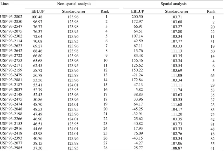
Table 4. Predictors (EBLUP) of individual genotypic effects of 28 soybean lines, respective standard errors and ranking of test

lines under two statistical analysis models(1)_.

(1)_{Grain yield data in kg ha}-1_{; variety trial with 110 lines and five checks, in augmented block design.}

Lines Non-spatial analysis Spatial analysis

EBLUP Standard error Rank EBLUP Standard error Rank

USP 93-2802 USP 93-2850 USP 93-2547 USP 93-2075 USP 93-2302 USP 93-2114 USP 93-2623 USP 93-2642 USP 93-2722 USP 93-2753 USP 93-2171 USP 93-2159 USP 93-2479 USP 93-2881 USP 93-2187 USP 93-2037 USP 93-2148 USP 93-2475 USP 93-2474 USP 93-2048 USP 93-2198 USP 93-2266 USP 93-2153 USP 93-2916 USP 93-2418 USP 93-2393 USP 93-2077 USP 93-2985 100.48 96.97 76.77 76.37 72.64 70.08 69.27 68.46 66.80 65.68 62.45 58.72 56.78 53.56 53.41 52.79 52.43 50.86 48.70 48.53 47.49 46.90 46.51 44.66 43.98 40.76 38.15 37.30 123.96 123.98 123.98 123.95 123.96 123.95 123.96 123.98 123.96 123.96 123.95 123.96 123.98 123.96 124.01 123.95 123.96 123.96 124.01 123.95 123.96 124.01 123.95 124.01 124.01 123.96 123.98 123.95 1 2 3 4 5 6 7 8 9 10 11 12 13 14 15 16 17 18 19 20 21 22 23 24 25 26 27 28 200.50 172.97 66.91 64.51 107.14 42.59 67.11 13.76 83.48 156.46 126.62 150.22 -21.24 172.84 47.13 5.82 38.83 33.96 64.17 -45.25 -32.91 25.62 -40.82 17.93 76.09 -43.15 -4.27 25.77 103.71 103.68 103.27 107.80 103.34 107.77 103.33 111.13 103.35 103.34 103.54 103.69 111.08 103.34 111.11 111.74 103.63 103.35 111.68 104.17 111.20 103.35 103.73 103.33 102.76 103.34 107.06 108.87 1 2 20 22 11 31 19 50 14 4 6 5 65 3 29 53 35 37 23 83 75 42 81 48 18 82 55 41 200 kg ha-1_{, in the spatial analysis the detected range}

was greater than 500 kg ha-1 _{(values between -337 and}

200.5). This represents an increase of more than 150% in the differentiation among the test lines, in favor of the spatial analysis. The smaller standard errors associated with EBLUP also confirm the better genotypic discrimination of this analytic model. Pontes (2002) has demonstrated a gain of 7% in the efficiency of these predictors when an iterative process to estimate the variogram and its parameters (a and σ2_{) was used.}

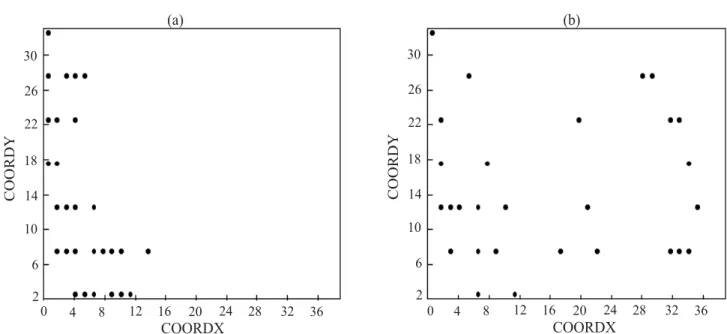
When a selection intensity of 25% of the most productive lines was assumed (28 in 110 genotypes), a coincidence of only 46% between the two statistical analysis models was observed (Table 4). In addition, among the genotypes selected by the more traditional analysis (non-spatial), at least 30% would occupy poor ranking positions in the spatial analysis (up to fiftieth position). Examples include the following lines:

USP 93-2048, USP 93-2393, USP 93-2153 and USP 93-2198. On the other hand, four lines classified in the spatial analysis as among the ten most productive would be discarded using the other analysis

(under R = I 2

e

σ ).

breeder’s preference in allocating genotypes of the same parent side by side. In any event, what is expected from experiments of this nature is an outcome as shown in part (b) of Figure 3 rather than one displayed in its part (a). Similar results are also reported by Besag & Kempton (1986), Cullis et al. (1989), and Kempton & Gleeson (1997).

Considering that the cause of the divergence in the two selections was the genotypic adjustment for position effects, which are of purely environmental nature, it can be concluded that, in similar conditions, the use of spatial analysis can assure greater efficiency to the breeding programs.

Conclusions

1. In variety trials with large numbers of treatments and limited availability of propagation material, experi-mental observations can not be spatially independent; in such conditions, spatial analysis allows better discrimination among genotypes, because it provides increased power in statistical tests, reduced standard errors of genotypic estimates, and greater amplitudes among predicted values.

2. The spatial analysis can be led to a different ranking of the genetic materials, in comparison with the non-spatial analysis, and a selection less influenced by local

variation; such differences may have important consequences for the final outcome of plant breeding programs.

Acknowledgements

To Dr. Natal Antônio Vello (Esalq, USP), who kindly provided the experimental data used in this study; to the Brazilian agencies Capes and CNPq, for the fellowships to first and second authors, respectively.

References

BESAG, J.; KEMPTON, R. Statistical analysis of field experiments using neighbouring plots. Biometrics, v.42, p.231-251, 1986. CULLIS, B.R.; LILL, W.J.; FISHER, J.A.; READ, B.J. A new procedure for the analysis of early generation variety trials. Applied Statistics, v.38, p.361-375, 1989.

DUARTE, J.B. Sobre o emprego e a análise estatística do delineamento em blocos aumentados no melhoramento vegetal. 2000. 293p. Tese (Doutorado) - Universidade de São Paulo, Piracicaba. <available on http://www.teses.usp.br>

ES, H.M. van; ES, C.L. van. Spatial nature of randomization and its effect on the outcome of field experiments. Agronomy Journal, v.85, p.420-428, 1993.

FEDERER, W.T. Augmented (or hoonuiaku) designs. Hawaiian Planter’s Records, v.55, p.191-208, 1956.

Figure 3. Location of plots with the most productive test lines (25%) among the 110 evaluated lines (unreplicated), using two

models of statistical analysis: with R = I σ2 _{(non-spatial) (a) and with R = Σ (spatial) (b) of a soybean variety trial, in augmented}

FEDERER, W.T. Recovery of interblock, intergradient, and intervarietal information in incomplete block and lattice rectangle designed experiments. Biometrics, v.54, p.471-481, 1998. GRONDONA, M.O.; CRESSIE, N. Using spatial considerations in the analysis of experiments. Technometrics, v.33, p.381-392, 1991. HENDERSON, C.R. Applications of linear models in animal breeding. Guelph: University of Guelph, 1984. 462p.

KEMPTON, R.A.; GLEESON, A.C. Unreplicated trials. In: KEMPTON, R.A.; FOX, P.N. (Ed.). Statistical methods for plant variety evaluation. London: Chapman & Hall, 1997. cap.6, p.86-100.

KEMPTON, R.A.; SERAPHIN, J.C.; SWORD, A.M. Statistical analysis of two-dimensional variation in variety yield trials. Journal of Agricultural Science, v.122, p.335-342, 1994.

LITTELL, R.C.; MILLIKEN, G.A.; STROUP, W.W.; WOLFINGER, R.D. SAS system for mixed models. Cary, NC: SAS Institute, 1996. 633p.

MARTÍNEZ, R. Control de la correlacion espacial en experimentos de campo en el sector agricola. Agronomia Colombiana, v.11, p.83-89, 1994.

PANNATIER, Y. Variowin: Software for spatial data analysis in 2D. Lausanne: Springer, 1996. 91p.

PONTES, J.M. A geoestatística: aplicações em experimentos de campo. 2002. 82p. Dissertação (Mestrado) - Universidade Federal de Lavras, Lavras.

SCOTT, R.A.; MILLIKEN, G.A. A SAS program for analyzing augmented randomized complete-block designs. Crop Science, v.33, p.865-867, 1993.

STROUP, W.W.; BAENZIGER, P.S.; MULITZE, D.K. Removing spatial variation from wheat yield trials: a comparison of methods. Crop Science, v.34, p.62-66, 1994.

VIEIRA, S.R. Uso de geoestatística em estudos de variabilidade espacial de propriedades do solo. In: NOVAIS, R.F. (Ed.). Tópicos em Ciência do Solo. Viçosa: SBCS, 2000. p.1-54.

WOLFINGER, R.D.; FEDERER, W.T.; CORDERO-BRANA, O. Recovering information in augmented designs, using SAS PROC GLM and PROC MIXED. Agronomy Journal, v.89, p.856-859, 1997.

ZIMMERMAN, D.I.; HARVILLE, D.A. A random field approach to the analysis of field-plot experiments and other spatial experiments. Biometrics, v.47, p.223-239, 1991.