Inflation Targeting did Make a Difference in Industrial Countries’ Inflation and Output Growth

Todos os direitos reservados.

É proibida a reprodução parcial ou integral do conteúdo

deste documento por qualquer meio de distribuição, digital ou

impresso, sem a expressa autorização do

REAP ou de seu autor.

Inflation Targeting did Make a Difference in

Industrial Countries’ I

nflation

and Output Growth

Ricardo Dias de Oliveira Brito

INFLATION TARGETING DID MAKE A DIFFERENCE

IN INDUSTRIAL COUNTRIES’ INFLATION

AND OUTPUT GROWTH

Ricardo Dias de Oliveira Brito

Ricardo Dias de Oliveira Brito Insper

Rua Quatá, nº300 Vila Olímpia

Inflation targeting did make a difference in industrial

countries

’ inflation and output growth

*

Ricardo D. Brito

Insper Institute of Education and Research

Associate Professor, Department of Economics E-mail address: RicardoDOB@insper.edu.br

Phone: 55-11-4504-2431; Fax: 55-11-4504-8415.

Postal address: Rua Quatá, 300, São Paulo, SP 04546-042, Brazil.

March 2012

Abstract

I evaluate the treatment effect of inflation targeting (IT) among industrial economies in the early 1990s, controlling for common time and country specific effects, to show that IT had significant enhancing effects on realized inflation and GDP growth. By additionally showing that IT lowered the long-term nominal interest rates, I indicate that IT worked through the expectation channel, meaning that IT was received as an improvement in monetary policy. This credibility bonus of pioneering IT regimes was economically important, significant and robust to sample and technique variations, providing support for policymakers’ optimism at the inception of the regime.

JEL classification: E31, E52; E58.

Keywords: Inflation targeting; Inflation; Inflation-output growth short-run tradeoff; Dynamic panel; Difference-in-difference; Propensity score matching

* _{For valuable discussion and help in understanding the data, I thank Eurilton Araujo, Rinaldo Artes, Cyntia}

Has inflation targeting (IT) made monetary policy more efficient in developed

economies? Have their pioneering IT systems, implemented in the early 1990s, resulted

in better realizations of inflation and output growth? Or, has IT subsequently spread

around the world just as a fad, without an initial track record of good performance?

Although the pioneering IT central banks seem happy with their choice, to the

point of having influenced the IMF recommendations and many other countries in a

subsequent wave of IT introductions after the mid 1990s, the existing evidence in terms

of realized inflation and output growth does not seem to support their optimism.1

Ball and Sheridan (2005) [denominated BS hereafter], for instance, put forth the

proposition that IT caused no significant improvement in realized rates of inflation and

output growth in a sample of major industrial economies. Although IT had a lowering

effect on inflation and a positive impact on GDP growth, they were not significant after

controlling these processes for mean-reversion in cross-section difference-in-difference

regressions. This view of IT irrelevance is shared by Lin and Ye (2007) [denominated LY

hereafter], who have found that IT had no significant effects on lowering inflation after

controlling for the self-selectivity bias of policy adoption in propensity score matches. 2, 3

In this paper, I demonstrate that IT did matter for realized inflation and output

growth. Through panel estimates of an adaptive Phillips curve that use data similar to LY

and BS, I show that the credibility bonus of IT policy amounted to a significant short-run

effect close to a 1 percentage point reduction in the annual mean inflation of inflation

1 _{King (2002) and Bank of Canada (2006) are two good examples of Central Bank(er)s optimism with IT.}

IMF (2006) is a document that pleads IT adoption.

2_{See Walsh (2009) for a survey of the IT literature. He concludes that ‘… macroeconomic experiences}

among both inflation targeting and non-targeting developed economies have been similar …’ (p. 195).

3 _{Studies like Geraats (1998), Roger and Stone (2005) and Crowe (2010) indicate that IT improved}

targeting countries (ITers), or a cumulative effect close to a 2 percentage point reduction

(in Tables 2 and 3). Although small compared to the worldwide inflation reduction

observed during the 1980s, it is relatively large and significant in comparison with

average inflation among industrial economies close to 2% per year in the late 1990s.

In these same samples, the impacts of IT on the volatilities of inflation and output

were negative, but mostly insignificant (in Table 4). Even so, given that inflation and

output growth rates had to undergo unavoidable volatility to converge to the new

long-run goals during the period studied, the fact that IT did not cause increases in volatilities

also shows IT effectiveness in improving macroeconomic performance at its inception.

To rule out the suspicion that this result spuriously reflects the role played by

supply shocks across the pre- and post-IT periods, and is in reality the consequence of a

more credible policy, I first show that similar results still hold when I allow for time and

cross-section heterogeneity in the inflation sensitivity to output growth (in Table 3,

columns (6) and (10)). Second, and more intuitively, I show that IT adoption significantly

lowered the long-term nominal interest rates, widely recognized as a proxy for long-run

inflation expectations (in Table 5).

What has caused this qualitative change in BS’s and LY’s IT irrelevance results,

distancing their results from my finding of IT enhancing effects?

In face of the generalized and sizable inflation reduction of the 1980s and early

1990s, IT’s absolute importance was second-order. However, once in the low inflation

regime of the 1990s, IT did play a significant role, which is not captured by BS, LY and

Instead of working with cross-section difference-in-differences or panel

propensity score matches – respectively used by BS and LY – which make it difficult to

model the short-run monetary tradeoffs and to control for common time variation and

countries’ non-observable specificities, I suggest a dynamic panel approach that exploits

the time and country dimensions to isolate the improvement in performance exclusively

due to the IT regime from other sources that might overlap in a cross-section. In

evaluating non-simultaneous IT treatment, it is particularly important to control for the

1980-90s’ worldwide trend of falling inflation and macroeconomic volatility.4 By

investigating the within-country variation, the control for country fixed-effects and for an

appropriate set of observable covariates addresses some of the omitted variable bias and

improves the inference about the causal effect of IT on economic performance. I choose

to model data at annual frequency and to identify the IT effects with a one-year lag,

together with other observable controls. The annual frequency is a simple solution to

minimize the autocorrelation of the residuals, while parsimoniously keeping the

estimated equations in the AR(1) family. The one-year lag of the explanatory variables

gives some time for the sluggish responses to monetary shocks of macro variables, in

accordance with Batini and Nelson (2002), and also weakens some endogeneity

suspicions of the IT policy.

Besides analyzing LY’s 1984-1999 annual balanced panel of 22 industrial

economies, combined with (i) BS’s calendar of IT adoptions or (ii) Mishkin and

Schmidt-Hebbel’s (2007) [denominated MSH hereafter] calendar of IT adoptions, I study: (iii) an

annual balanced panel that extends LY’s data back to 1971, (iv) an annual unbalanced

4 _{See Cecchetti et al. (2006) for a cross-country study about the worldwide trend in the 1980-90s of falling}

panel that covers BS’s sample of 20 industrial countries between 1985-2001, and (v)

another unbalanced panel with BS’s economies between 1980-2009. In all samples, I

have been able to show that the IT policy improved realized inflation and output growth.

Having overturned BS’s and LY’s conclusions of IT irrelevance, I then revisit

both studies. First, by subtracting the common time and country fixed effects from the

variables of interest, then running BS’s cross-section difference-in-difference regressions

with these mean-deviation transformed variables, I am able to show that IT significantly

lowered inflation, increased output and lowered long-term interest rates, in an example of

Ball’s (1994a) credible disinflation. Second, by reformulating LY’s propensity score

matching to fulfill the conditional independence assumptions (CIA) – of (i) one unit of

treatment per ITer and (ii) matching of observables before treatment, violated by LY –

once again, I reach the conclusion that the IT framework resulted in significant

improvements in the realizations of inflation and output growth among industrial

countries.

In sum, this paper reveals that the initial track record of IT was significantly

positive, in support of policymakers’ optimism, and thus justifying its spread around the

world after the mid-nineties.

The article is organized as follows. Section 1 compares the panel regression

methodology with the cross-section difference-in-difference regression and the PSM

techniques, showing that the linear dynamic panel procedure controlled for the right set

of covariates is a more suitable approach in contexts where short-run tradeoffs and

non-observables matter. Subsection 2.1 reports and discusses the main results. Ball and

2.3. The conclusions are in section 3, and the data sources and various samples used are

described in Appendix A.

1. Methodology

1.1. Linear Regression

I first work with a partial adjustment model:

y t n y n y t t n y IT

t n y t n y t

n y d X

y _,   _,1  _,1  _,1   _, , (1)

where: yn,t is some macroeconomic performance indicator of interest; subscript n = 1,

2, …, N is for country; and t = 1, 2, …, T is for period in years. For concreteness, I will

sometimes refer to yn,t as “inflation” of country n in year t , but similar reasoning can

be applied to other indicators of macroeconomic performance, such as real output growth,

inflation volatility or output growth volatility. The lagged value yn_,t₁ on the right-hand

side captures persistence and mean-reverting dynamics. Among the independent

variables, my focus is on the IT dummy variable IT t n

d _,1 , equal to 1 if country n is an

inflation targeter in period t-1 and 0 if it is not. Hence IT t n

d _, is the treatment variable.

The one year lag gives time for policy to transmit to the economy (for treatment to take

effect). The vector Xn_,t₁ accounts for other covariates. For example, when y refers to

inflation, Xn_,t₁ can include GDP growth, among others. The term

y t

effects that capture common shocks to all countries, y n

 allows for cross-country fixed

effects, and y t n,

 is the disturbance. The vector y



y y y



, ,

 of common

coefficients has y

as the main parameter of interest for evaluation of IT policy

effectiveness.

BS’s model can result from the time degeneration of equation (1), which sums up

all the data available into t = pre-IT, post-IT periods, thus turning the (T-1)-period

dynamic panel (1) into a cross-section:

n e

X d

y

y nypost

y pre n y IT

post n y pre n y post

n,   ,   ,   ,   ,  ,

where: yn,post is country’s n post-targeting average inflation value, yn,pre is its

pre-targeting value, and en,post



n n,post



. By subtracting yn,pre on both sides of the

above equation, BS estimate:

n e

X d

y y

y_n,post _n,prey' _n,prey _nIT_,posty _n,prey  _ny_,post  , (2)

with y'



y 1



.

In equation (2), it makes sense that the treatment variable IT post n

d _, is

contemporaneous with the dependent variable yn,post , given that IT

pre n

d _, is always zero.

The necessary time lag for treatment to transmit to the economy is not a concern in the

mean or the standard deviation) over many post-treatment years. However, equation (2)’s

parameter estimates may be biased because of the omission of the time-effect variation

y t

 and the impossibility of identifying the country-effect variation y n

 from y post n

e _, .

As Bertrand et al. (2004) point out, to ignore the time series information of the

datawould work well only if all targeters had adopted the regime at the same time. Then,

the periods covered by pre-IT and post-IT windows would be the same for every

country, incorporating exactly the same combination of time-effect variation, and

cancelling out in a between-country comparison. But since IT adoption happened at

different times for different economies, the pair of pre-IT and post-IT periods are not

the same for all ITers and have to be arbitrarily defined for non-ITers. This means that

the time-effect variation t cannot be ignored in the IT analysis.

Apart from the common time-variation problem, BS’s cross-section regression

would be useful to investigate the between-country variation, which is to ask whether

targeters have lower inflation. However, equation (2) also ignores unobserved

country-specific factors affecting both inflation dynamics and IT adoption, and may erroneously

suggest a causal relationship from IT to inflation. To investigate the “within-country”

variation, which is to ask whether a country is more likely to have a lower inflation in

case it adopts the IT framework, it is necessary to control for country-specific observed

and non-observed factors affecting both inflation and IT adoption. In addition to the

inclusion of appropriate covariates Xn_,t₁ in the regressions, this control can partially be

accomplished by the use of country-effects y n

 , like in equation (1). Although y n

 does

not control for the time variation of those country-specific non-observable factors, it

Regarding the estimation method of equation (1), the LSDV (least square dummy

variable) estimator may have a bias when T is small, as demonstrated by Nickell (1981).

With big N and small T, the Difference GMM of Arellano and Bond (1991) would be

advisable. However, Judson and Owen (1999) and Roodman (2008), among others,

indicate the weak instruments and over-fit risks of applying these techniques to panels

with small N relative to T. Judson and Owen (1998) additionally show that LSDV

performs well when N is small and T increases. Bruno (2005) develops a correction of the

LSDV estimator for panels, but that approach is only valid for strictly exogenous

regressors. Thus, in the absence of a best technique to handle this small N panel with

weakly exogenous regressors, I choose to present estimates from both the LSDV

estimator and Difference GMM.

The LSDV, or fixed-effect OLS estimator, is biased if the transformed

independent variables







,1 , 1



1 1

, *

1

, 1 ... 

 

  nt   n   nT t

n y T y y

y and







,1 , 1



1

1 , *

1

, 1 ... 

 

  n t   n   nT t

n Z T Z Z

Z , for _,1 



_{, 1}, n_,t_1



IT t n t

n d X

Z , are correlated with

the transformed error







y



T n y n y t n y t

n T ,2 ,

1 ,

*

,  1  ... 

      

. The correlation between

* 1 ,t n

y and y_,* t n

 has been shown by Nickell (1981) to be negative, resulting in a

downward biased estimator of y

, known as the dynamic panel bias problem, which

shrinks as T gets larger.

The biases in the



y y



, LSDV estimators of (1) depend on the covariances



y



j t n t n

Z _{, 1}, _{, }

cov  for all t 2 and j = 1, …, (t - 2). Specifically for the inflation-IT



,



0 cov _,₁ n_,tj 

IT t n

d , meaning IT

t n

d _,1 is predetermined. After all, IT adoption is

generally motivated as a way of “improving” the inflation process behavior. Less clear at

this point is the sign of



nt j



IT

t n

d _,1, _,

cov . While BS argue that countries with higher past

inflation tend to adopt IT, LY show (and I confirm in Table 7 below) that switches to the

IT regime are more probable when inflation is already low. This latter being the case, the



,



0 cov _,₁ n_,tj 

IT t n

d for t 2 and j = 2, …, (t - 2) would bias the  LSDV

estimates of (1) upwards, thus making it more difficult to find that IT decreases inflation.

Even so, to confirm the sign and significance of the IT effects, I additionally present

Difference GMM estimates that treat the Zn,t1 explanatory variables as strictly

exogenous, and also as predetermined ones.

Because serially correlated residuals might cause the standard error for the

estimated y

to severely understate the standard deviation of population y , as

Bertrand et al. (2004) have shown, I cluster the standard errors by country and report

tests of whether the error term y t n,

 is serially correlated. The assumption that the error

terms are not serially correlated is equivalent to their first-differences y t n,



 being

first-order correlated but not second-first-order correlated.

1.2. Propensity score matching

In the above equations (1) or (2), the estimated y

is intended to represent the

average direct causal effect of IT on y over all years and all ITers. However, this is only

exact if all confounding variables have been properly included in the model and if the

control units. In other words, regression-based causality tests assume a simple CIA to

assure that treated and non-treaded subjects in the sample become comparable and there

is no selection bias.

Because a regression-based conditional independence test relies on a model of the

process determining inflation (or other macroeconomic variable), it implies auxiliary

assumptions that may be hard to assess and interpret. Hence, alternative tests able to relax

those assumptions are worth considering. Assuming that assignment to treatment only

depends on observable variables – and does not depend on non-observables – the

propensity score matching (PSM) approach is an alternative that is more focused on the

estimation of the propensity score of policy adoption,



n pre n pre





n pre n pre



IT post

n y X p y X

d

E _, | _, , _,  _, , _, , where p



y_n,pre,X_n,pre



is the conditional

probability of IT adoption, instead of on the model for outcomes,



n pre n pre



IT post n post

n d y X

y

E _, | _, , _, , _, . According to Angrist and Pischke (2009), this is attractive

in applications where the former is easier to model or motivate, while by leaving the

model for outcomes unspecified, PSM should increase robustness.

LY and Vega and Winkelried (2005) follow this approach, emphasizing they

address the self-selection problem of IT policy adoption ignored by BS and others. Not

explicit in their argument, though, is that it is the control for X_n,pre , and not the PSM

framework itself, which minimizes the selection bias. Although PSM provides a robust

measure of the conditional expectation function (CEF), given that regression also

approximates the CEF, differences between the PSM average treatment effect on the

treated (ATT) and the regression y

unlikely to be of major empirical importance. As Angrist and Pischke (2009) show, in a

cross-section context both can be motivated as a weighted matching estimator:





_





_

_

_





_

_

                     pre n pre n pre n pre n post n pre n pre n IT post n pre n pre n X y p X y p y X y p d X y g E , , , , , , , , , , , 1 , , , ,

where g



y_n,pre,X_n,pre



is a known weighting function. For the PSM ATT ,



 

_

_



1 , , , , , ,

,  IT _

post n pre n pre n pre n pre n d p X y p X y

g , meaning that PSM weights are proportional to the

probability of treatment at each value for the covariates. For the y

regression,





_



_



_



_



_





_

_

_

_



_



_

_

pre n pre n d pre n pre n d pre n pre n pre n pre n pre n pre n pre n pre n pre n pre n X y E X y X y p X y p E X y p X y p X y g IT IT , , 2 , , 2 , , , , , , , , , , , , , 1 , , 1 , ,       

 , meaning

that regression weights are proportional to the variance of treatment at each value for the

covariates.5 Thus, it is BS’s and others’ lack of control for X_n,pre in the estimation of

equation (2) that may impair the results of the previous literature, rather than the linear

regression approach.

Further, as noted by Dehejia and Wahba (2002): “An important issue is whether

the assumption of selection on observable covariates is valid, or whether the selection

process depends on variables that are unobserved ... Only when the researcher is

comfortable with the former assumption do PSM methods come into play.” In the IT

literature, the propensity score of IT adoption is far from well understood and the

assumption that the political macroeconomic decision of IT adoption is not affected by

5 _{Note that for the average treatment effect (ATE),}



_,



₁ , ,pre n pre 

n X

y

common-time and country-fixed non-observables seems too strong, given the cluster of

IT adoption in the beginning of the 1990s, and that the inflation process that IT seeks to

control is affected by common-time and country-fixed effects. The above points make

clear that PSM has drawbacks in the IT context, and is thus best advised as a

complementary exam rather than a superior technique.

Ignoring the plausible common time-variable and country fixed effects, to better

understand LY’s results, it is enlightening to describe how the PSM would work well in a

panel context. However, this is complicated by the fact that potential outcomes are

determined not just by current policy actions but also by past policy actions and

covariates. Given that ITer ni adopts the IT treatment from the year kni on, i.e. for

T t

k_ni  ' , dIT_,' 1 t' t

ni   , to measure the average causal effect of IT on the outcome variable

n i

k h n

y _{, } after h years of treatment, the researcher would have to compute:



0 | _, 1



, 1

,  

 nihk nihk niIThk

h E y ni y ni d ni

ATT ,

where 1 ,h kn i

ni

y _ is the outcome in period



hkni



if country ni adopted IT and

0 ,h kn i

ni

y _

if not.

However, because the outcome that would have been observed if ITer ni had not

adopted IT policy 0 | _, 1

,   

IT k h ni k h

ni ni d ni

y is not observable, the researcher assumes that

potential outcomes are independent of treatment status, conditional on a scalar function

of covariates, i.e. the CIA





,



, 1 , 1



0 , 1

, n, n  n| nkn, nkn

IT k h n k h n k h

n y d p y X







, , 1 , 1



0

, ni | ni 1, nikni, nikni

IT k h ni k h

ni d p y X

y

E by observable



 





, , 1 , 1 , 1 , 1



0

, ni | ni 0, nkni, n kni  nikni, nikni

IT k h n k h

n d p y X p y X

y

E , and equivalently measures:







 



, , , , 0 | , , 1 | 1 , 1 , 1 , 1 , , 0 , 1 , 1 , , 1 ,                                ni ni ni ni ni ni ni ni ni ni k ni k ni k n k n IT k h n k h n k ni k ni IT k h ni k h ni h X y p X y p d y E X y p d y E ATT

or its sample analogue:



 













            IT ni ni ni ni ni ni ni N ni k ni k ni k n k n IT k h n k h n k h ni IT

h y E y d p y X p y X

N ATT 1 1 , 1 , 1 , 1 , , 0 , 1

, | 0, , ,

1

,

where N_IT is the number of ITers.

If, additionally, one assumes, as LY does, that common-time varying effects do

not affect the outcomes, or the common-time varying effects have been extracted from

the outcome series, there is no need for the treatment and controls outcomes to occur at

the same time, and for any 



Th



, the above equations can be rewritten as:







 



_                             1 , 1 , 1 , 1 , , 0 , 1 , 1 , , 1 , , , , 0 | , , 1 | ni ni ni ni ni ni k ni k ni n n IT h n h n k ni k ni IT k h ni k h ni h X y p X y p d y E X y p d y E ATT     , or



 













          

 NIT _{ni ni ni}

ni k ni k ni n n IT h n h n k h ni IT

h y E y d p y X p y X

N ATT 1 1 , 1 , 1 , 1 , , 0 , 1

, | 0, , ,

1

  

However, to measure the cumulative ATT over



H 1



years in a panel context,

one has to average the ATT_hs :









  H h h H ATT H ATT 0 1

1 ₍₄₎



1



1





| 0,



,

 

,







,

1 0 1 1 , 1 , 1 , 1 , , 0 , 1 ,





              H h N ni k ni k ni n n IT h n h n k h ni IT IT ni ni

ni Ey d p y X p y X

y N

H    

which, for the biggest H possible, approximates the cross-section ATT measure over all

post-treatment years, usually calculated in the PSM literature:6







 



_                   pre ni pre ni pre n pre n IT post n post n pre ni pre ni IT post ni post ni post X y p X y p d y E X y p d y E ATT , , , , , 0 , , , , 1 , , , , 0 | , , 1

| , (5)

that is the PSM analogue of the cross-section difference-in-difference y .

LY’s PSM results are flawed because, when attempting to compute (4), they

ignore that the year of IT adoption kni is a definite and fixed one for each country for

exogeneity to be preserved. Instead of conditioning on



_{, 1}, _{, 1}



ni ni nik

k

ni X

y

p for every

horizon h0 , LY condition on





ni ni nih k

k h

ni X

y

p _{,  1}, _{, } , and compute the measure:

6 _{Vega and Winkelried (2005) use equation (5) to evaluate the IT policy. However, although they analyze}

industrial ITers’ performance separately, they do it against a control group that includes both industrial and emerging economies, thus not restricting the comparison group to units that are similar to the exposed ones,







,

 

,



, , 0 | 1 1 1

0 1 , 1 , , 1 ,

, 0 , 1 ,







                              

 ni IT

ni ni ni k T h N

ni nh nh nih k nih k

IT h n h n k h ni IT

ni p y X p y X

d y E y N k T LYATT    

thus matching on observables that have already been influenced by previous h years of

treatment. Just taking into account the conditioning variables yn_,h₁ and yni,hkni1 , for

illustration, LY are matching the treated outcome after h years of treatment 1 ,h kni

ni

y _

with non-treated 0 ,h

n

y ’s, not because they were similar before treatment started (h+1)

years ago, y_{ni,k 1}y_n,1

ni , but because they were similar last year, after (h-1) years of

treatment, y_{ni,hk 1}y_{n,h1}

ni . This violates the exogeneity assumption for h>0 , and

clearly results in underestimation of the treatment effect through time.

2. Results

Next, in subsection 2.1, I present the linear regression results. As explained in

section 1, a dynamic panel that controls for observable covariates is as able to address the

IT causal effect on inflation as the PSM, with the advantage of taking relevant

non-observables into account and making explicit the roles of past policy actions and

observable covariates in the inflation determination (or in another macroeconomic

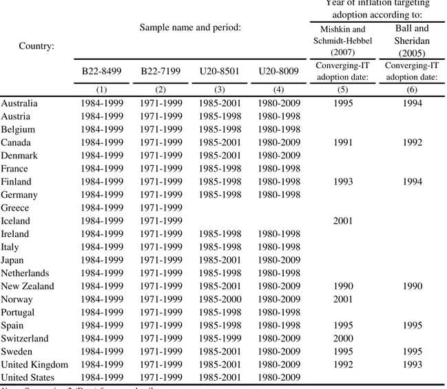
variable). The samples used are described in Table 1 and detailed in Appendix A.

To make sure that the main results I obtained in subsection 2.1 are not technique

sensitive, in subsections 2.2 and 2.3 I show that similar qualitative results could have

been obtained by cross-section difference-in-difference and PSM, had BS and LY

< Insert Table 1 around here >

2.1. Main Results

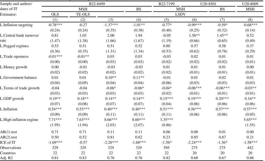
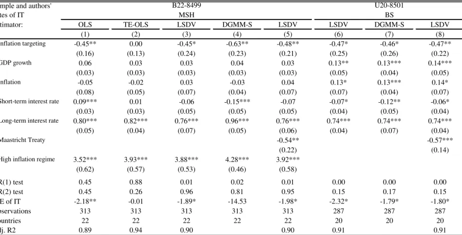
In Tables 2 to 5, I show estimates of variations of equation (1), presented in

section 1. Table 2 presents estimates of the following adaptive Phillips curve with a set of

controls: . ) 6 ( 5 , 1 , 1 , 1 , 1 , 1 , 1 , 1 , 1 , , 1 , ,                           t n n t t n ttg t n gdpg t n fix t n cggdp t n cbturn t n bmg t n open IT t n IT t n t n TTG GDPG FIX CGGDP CBTURN BMG OPEN d                              

Beyond the current and lagged inflations (n,t and n,t1), GDP growth

(GDPGn_,t_1), and terms of trade growth (TTGn,t1) – usual variables in an open economy

adaptive Phillips curve 7 – following Ghosh et al. (2002) and LY, I include other

potential determinants of inflation to certify that the IT effect shows up in a very

controlled model.

According to Romer (1993), greater trade openness (OPENn,t1) should imply

lower inflation, given the higher costs of a monetary expansion. Faster growth of the

money supply (BMGn,t1) should trivially be associated with higher inflation. Cukierman

(1992) argues that a higher turnover rate of the central bank governor (CBTURN5n_,t₁)

should be associated with higher inflation. By its importance in aggregate demand, higher

7 _{See Hutchison and Walsh (1998), Andersen and Walsher (1999), Mankiw (2001) or Mehra (2004) for}

government surplus (CGGDPn,t1) should alleviate pressures to raise prices. Ghosh et al.

(2002) also introduce a dummy for pegged exchange rate regimes (FIXn_,t_1) and find that

these regimes presented lower average inflation worldwide.

<Insert Table 2 around here>

The first 4 columns of Table 2 show estimates for sample B22-8499 (described in

Table 1, column (1)) with Mishkin and Schmidt-Hebbel’s (2007) [denominated MSH

hereafter] calendar of IT adoptions (described in Table 1, column (5)). This is the sample

that gets more attention in this paper, not only because it was the sample used by LY,

with whose results mine differ, but also because it is a balanced panel that covers the

inception of the IT system. After 1999, 11 of these 22 industrial countries unified their

monetary policy under the European Central Bank, making it debatable whether they

should be analyzed as independent countries from then on. MSH’s IT adoption dates are

the closest to Bernanke’s et al. (1999) country-case studies and the IMF’s (2006). They

also better represent the common central bank operating procedure of starting an IT

regime with explicit targets for the coming year on rather than for the current year, as

described in Johnson (2002).

I present pooled cross-sectional OLS estimates in column (1), including the

common time-variable effect in column (2), and the common-time-variable and

country-fixed-effects in column (3). From the changes in coefficient estimates among these 3

columns, it can be seen that the common-time-variable and country-fixed effects do

affect inflation. The IT impact is already significant in the simplest model in column (1).

Although IT becomes less important with the inclusion of the common-time effect, it

showing that non-observables play a role in the inflation process. Both the direct impact

of IT on inflation,  , and its cumulative effect, 



1



, which accounts for

subsequent decreases over-time lagged inflation on the right-hand side, are significant.

Columns (3) to (8) of Table 2 present panel estimates with time and fixed-effects

for the various samples and two calendars of IT adoption described in Table 1. From

column (3) to (4), I change from MSH’s to BS’s IT calendar – the one used by LY – to

check how important it is to vary the dates of IT adoption. The different calendars of IT

adoption make a quantitative difference, but not important enough to change the

qualitative result that IT mattered. BS’s IT adoption dates reduce the IT direct impact on

the average inflation level from -1.37 to -1.01 percentage points, or its implied

cumulative effect from -2.28 to -1.68 percentage points. Anyway, the IT effect is still

significantly important, different from LY’s irrelevance conclusion (in their Table 3,

Panel A), and differences between columns (3) and (4) mainly reflect that my

identification strategy of a one-year lag in policy effects matches better with MSH’s

calendar.

In column (5), the balanced panel B22-7199 extends B22-8499 back to 1971 to

reduce the dynamic panel bias problem suspicion and to check if the IT effect is still

important when observed in a longer retrospect. The direct effect of IT is -0.77

percentage point, lower than the -1.37 percentage points from column (3), but is still

significant at 6% significance.

The estimates in columns (6) to (8) are based on U20-8501 and U20-8009

(described in Table 1, columns (3) and (4)). They are unbalanced panels of the 20

al. (2002) (as described in Appendix A). The results in column (7) are comparable to

BS’s IT irrelevance findings (in their Table 6.3), given that BS’s IT adoption dates are

used in it. From the comparison of columns (6) and (7), again, it becomes clear that the

combination of the one-year lag in policy effects with BS’s calendar captures less of the

IT effect than MSH’s calendar, but it is still significant.

Although smaller than column’s (6) estimates for data until 2001, in column (8),

the IT coefficient presents significant enhancing effects on inflation until 2009, meaning

that the average disinflation gain of the IT policy is still noticeable many years after its

introduction. Among many, one possible explanation for the reduction in size of the IT

effect is that non-explicit IT central banks incorporated best IT practices during the

2000s, as indicated by Geraats (1998), among others.

Regarding the goodness of fit statistics, in accordance with the assumptions, there

is no evidence of first-order autocorrelation of the residuals in the equations tested in

levels (OLS and TE-OLS, in columns (1) and (2)), or of second-order autocorrelation in

the equations tested in differences (LSDV, in columns (3)-(8)), respectively represented

by the p-values of the AR(1) and AR(2) test statistics. Besides weakening suspicion that

the significances found are the spurious result of autocorrelated residuals, these tests

show that the one-year period frequency suits the AR(1) model parameterization well.

If one agrees that the set of variables controlled for by LY is just the right set of

covariates, their inclusion in regression (6) is enough to interpret the IT-inflation

regression relation as a causal one as well. In the inflation-output tradeoff context of the

Phillips curve, this IT effect is what monetary economists call the “credibility bonus”, or

turnover rate is only significant in the 1985-2001 unbalanced panels, but even there it

does not obviate the IT effect.8 If CBTURN5n,t1 is a good proxy for central bank

independence, the results in Table 2 allow the conclusion that IT was effective in

lowering inflation, and its impact was in addition to central bank independence.

Further, with respect to columns (3) to (8) of Table 2, it can be seen that besides

lagged inflation, output growth and terms of trade growth, the usual characters in an

adaptive open economy Phillips curve, the IT dummy is the only variable that is

significant in all seven samples. The variables for exchange rate regime, trade openness

and broad money growth were rarely significant. The government balance surplus

(CGGDPn_,t_1) is significant for the samples that cover the period 1984-1999, but with a

positive sign that is opposite to that expected, and it becomes insignificant in column (6),

which just extends the same vintage of data back to 1971.

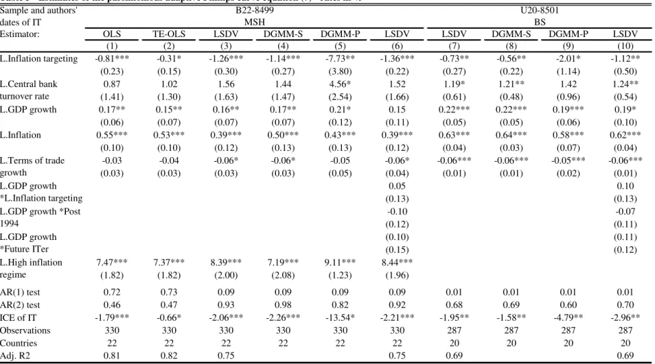
In Table 3, I exclude the variables that were not useful in explaining inflation in

Table 2, and return to a more parsimonious adaptive Phillips curve, where:

; 5 , 1 , 1 , 1 , 1 , , 1 , ,                   t n n t t n ttg t n gdpg t n cbturn IT t n IT t n t n TTG GDPG CBTURN d                   (7)

8 _{The significance of CBTURN5 in sample U20-8501 might be the consequence of two facts. First, as}

with the CBTURN5n,t1 kept in the equation to isolate the IT regime from other

observable differences of the central bank. 9

<Insert Table 3 around here>

The IT effects shown in Table 3 only change slightly from the pattern of Table 2,

generally becoming stronger and more significant. In columns (1) to (3), I again show

how non-observables affect the inflation process. Once again, different from LY’s

irrelevance conclusion, column (3) presents significant IT accomplishments, and the IT

effects are stronger in column (7), in contrast with BS’s irrelevance conclusion.

To analyze how serious the dynamic panel bias problem is, in columns (4) and (8)

I show Difference GMM estimates that treat the Zn,t1 covariates as strictly exogenous

(DGMM-S). Note that the autoregressive coefficients are not significantly different from

their LSDV pairs (respectively in columns (3) and (7)), and that the IT effect does not

change significantly either. Because it is reasonable to suspect that past inflation shocks

feed back into future realizations of the other explanatory variables, I also show

Difference GMM estimates with Zn_,t₁ predetermined explanatory variables (DGMM-P

in columns (5) and (9)). In spite of some loss of precision and unreasonably large

absolute sizes for the IT coefficients, caused by over-fitting (too many moments relative

to countries), the IT effect remains significant.

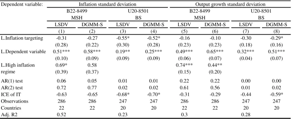
<Insert Table 4 around here>

9 _{I am aware that, in the intuitive case where successful IT adoption increases central bank independence}

In Table 4, I estimate the IT achievements on the inflation and output growth

volatilities, as in equation (1), obtaining results that are comparable to those of BS’s and

LY’s tests. The inflation and output growth standard deviations went down because of IT,

although not as much as the inflation levels. Given that most countries were going

through unavoidable volatility to lower their long-run mean inflation, the fact that IT

adoption did not cause an increase in volatility is actually evidence of IT’s improvement

in macroeconomic performance.

To rule out the suspicion that the results presented so far spuriously reflect a

relatively more important role played by supply shocks across the pre- and post-IT

periods, and to confirm it is truly the consequence of a more credible policy, I first show

that similar results hold when I allow for time and cross-section heterogeneity in the

inflation sensitivity to output growth. In columns (6) and (10) of Table 3, I make the

output growth interact with (i) the standard IT dummy, nt

IT t

n L.Inflationtargeting

d _{, 1}  _, ;

(ii) a dummy variable equal to 1 for all countries in every period t after the average

year of IT adoption, Post1994n,t ; and (iii) a dummy variable equal to 1 for all years in

every country n that adopts IT, FutureITersn,t. The fact the IT intercept is still

negative and significant when the inflation responses to output are allowed to be different

between ITers and non-ITers (L.GDP growth*Future ITers), to vary across pre- and

post-IT periods in general (L.GDP growth*Post 1994) and to change after IT adoption for the

ITers (L.GDP growth*L.Inflation targeting), excludes spurious effects of decreases in the

variance of supply shock that may have occurred at different times in the different

Second, and more intuitively, I study the impact of IT on the nominal long-term

interest rate process, believed to be a proxy for long-run inflation expectations. Because

the nominal long-term rate reflects not only expectations of future inflation, but also

future activity levels, monetary policy tightness and the risk premiums related to those

factors, I model it as:

; , 1 , 1 , 1 , 1 , , 1 , , L t n L n L t t n L t n L gdpg t n L short IT t n IT L t n L t n GDPG short d long long                             (8)

where: long is the nominal long-term interest rate and short is the nominal short-term

interest rate.10 In Table 5, as in the inflation case, the IT lowering impact on the long rate

is already significant by simple OLS in column (1) and, although it becomes unimportant

with common-time effects in column (2), it confirms its significance when the

country-fixed effects are also included. IT had a significant direct impact on the average

long-term interest level of around -0.5 percentage point in columns (1), (3) and (6), or an

implied cumulative effect close to -2.00 percentage points, in spite of the simultaneous

decrease in risk premiums happening among future Euro members.11 The results are

similar for Difference GMM, although the autoregressive coefficient seems

overestimated in column (4). When I additionally control for the Maastricht Treaty effect,

the IT effect becomes even more significant in columns (5) and (8).

<Insert Table 5 around here>

10 _{I thank Niamh Sheridan for providing the nominal long-term interest rate data used in BS.}

It is worth noting that the results presented so far are not incoherent with Brito

(2010), who, in a debate with Gonçalves and Carvalho (2010), shows that IT disinflations

were not less costly in the OECD. They discuss Ball’s (1994b) disinflations, i.e. events in

which the nine-quarter moving average of inflation went down by more than 2%, when it

is better to have a lower output-loss-to-inflation-reduction ratio, called output sacrifice

ratio. However, a lower output sacrifice ratio in Ball’s (1994b) context is not a necessary

or a sufficient condition for a policy to be considered more efficient in general, when not

only sizable disinflations but the whole business cycle has to be handled by monetary

policy. In other words, the fact that IT did not matter for “big” disinflations does not

imply that IT does not matter at all. And, indeed, the 2% cut-off used in these studies is

too coarse for the already low OECD inflation levels at the IT inception. Instead, given

the OECD economies adopted IT more as a regime to fine tune the whole business cycle

than a transient mean to disinflate, the current paper evaluates the average effect of the IT

treatment on inflation and output, conditional on their continuing tradeoffs and on other

covariates.

Nevertheless, the current paper’s findings are qualitatively different from those of

Brito and Bystedt (2010), who conclude that IT rendered no credibility bonus among

emerging economies. According to Brito and Bystedt (2010), the emerging ITers’ relative

inflation reduction was the compensation for their relatively lower output growth. Given

the early 1990s’ prevalent gap in credibility between industrial countries’ monetary

authorities and those of emerging economies, both papers’ results put together seem to

illustrate Ball’s (1995) imperfect credibility theory, where inflation control costs less for

(2005) and Mishkin’s (2000) suspicions that IT works better in already strong

institutional environments, and is thus not a panacea for emerging economies.

2.2. Ball and Sheridan (2005) Revisited

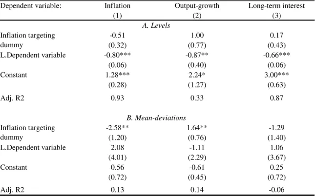
In Table 6, I revisit BS’s 20 country cross-section difference-in-difference

regressions. First, to show that their methods with my data also produce the irrelevance

result for IT, I present estimates by equation (2) for inflation, GDP growth and long-term

interest rates, respectively in columns (1) to (3) of panel 6.A, which are comparable to

columns (6) of BS’ Tables 6.3.B, 6.6.B and 6.8.B. In percentage points, the IT impacts

are close to -0.50 on inflation, 1.00 on output growth and 0.20 on the long-term interest

rate, all insignificant at 10% significance level, as in BS.12

<Insert Table 6 around here>

Second, in an attempt to control for common-time-variable and country-fixed

non-observables, I subtract these effects from the variables and re-estimate equation (2)

in panel 6.B. Even though the cross-section difference-in-difference set-up does not

permit accurate control of the processes’ short-run dynamics and tradeoffs with other

observable covariates, the IT effects become economically important. The IT

simultaneous enhancing effects to relative inflation and relative output growth confirm

the credibility bonus, suggesting additionally a context of relatively perfect credibility

close to Ball (1994a), where (relatively) credible disinflations can cause (relative)

economic booms.

12_{Although I used BS’ data for the nominal long-term interest rate, I do not get their result exactly (0.17}

2.3. Lin and Ye (2007) Revisited

As explained in section 1 (and detailed in Appendix C for the referee’s benefit),

LY’s PSM application to a panel is not standard. Instead of one unit of treatment per ITer

(7 countries), they consider every year-country under IT as an independent unit to be

treated (totaling 45 events). Next, they match these units by their contemporaneous year

observable characteristics, instead of by their pre-treatment characteristics, and base their

evaluation on that same year inflation,











,



, 1 ,

 

, '1 ,'





0 , '

, 1 ' , '

, 1

'

, | 1, , | 0, n , n nit , nit

IT n n t

ni t ni IT

t ni t

ni d p X E d p X p X

E   _   _{ }   _{ }   _ for all

ni

k

t' and  , including

 

t'1 k_ni . By violating the CIA, LY’s results are subject to

the selection bias they propose to solve. The fact that current ITers have (or do not have)

current lower inflation rates, as measured by LY, is not conditional on ITers and matched

controls being similar before IT adoption. In other words, for the purpose of inferring the

IT treatment effectiveness, it does not imply that a country is more (or less) likely to

lower its inflation if it becomes an ITer.

<Insert Table 7 around here>

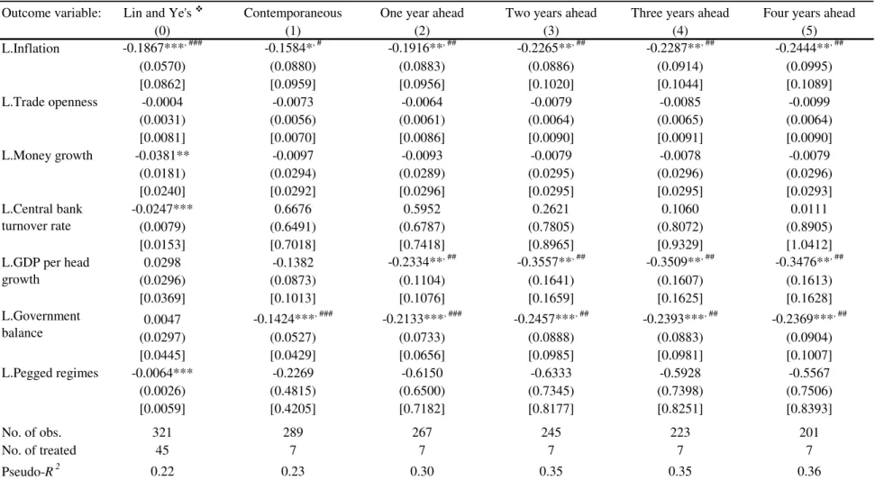
In Table 7, I reformulate LY’s Probit model of IT adoption (replicated in column

(0); or in Table C.1 for the referee’s benefit), fulfilling the requirements of: (i) one unit of

treatment per ITer and (ii) matching of observables before treatment, but keeping their

panel structure and the set of covariates. To calculate the probability of IT adoption,

instead of the probability of being an ITer calculated by LY, ITer observations are

included in the Probit estimation only if the country had not adopted IT previously, for

ni

k



 – i.e., ITers observations are not used in the Probit estimation after the first year

for by LY are lagged by one year, p



n_,₁,Xn_,₁



instead of p



n,1, Xn,



. Finally,

because I will match at horizon h , I need the outcome variable to exist at year



 h



and have to avoid ITers’ outcomes already under treatment from becoming controls for

themselves. I thus drop the observations of all countries dated  



T h



and the

observations of pre-treatment ITers’ years from which the term h ends up in their

treatment periods. These two latter precautions generate a different subsample and its

respective Probit for each horizon h .13

From sample B22-8499 combined with BS’s IT calendar (my equivalent of LY’s

sample), where the last IT adoptions happened in 1995, it is possible to compute the

h

ATT for h=0, 1, 2, 3, 4 . In Table 7, from columns (1) to (5), I present the IT adoption

Probit estimates,



_, |n_,₁, n_,₁







n_,₁, n_,₁



IT

n X p X

d

E , for each of these five

subsamples.14 In the Probits, the explanatory variable last-year inflation has a negative

and significant impact on IT adoption, meaning that countries with lower inflation are

more likely to adopt IT. This is in accordance with LY, but runs counter to BS’

assumption that IT adopters had higher inflation, at least on the eve of IT adoption.

Among the seven observables studied by LY, inflation was the only one they lagged and

is the only one that has preserved its sign and significance. Compared to LY’s Table 2,

broad money growth, central bank turnover and pegged exchange rate regimes are now

13 _{For illustrative purposes, take as examples the sample B22-8499, the inflation difference two years after}

IT adoption ₂ 



1_, ₂| _, 1,



 _, ₁, _, ₁









0_,₂| _, 0,



n_,₁, n_,₁





IT n n k

n k n IT

k n k

n d p X E d p X

E

ATT , and

Sweden’s IT adoption in year kni=1995 . Because _n,2| p



_n,1,X_n,1



does not exist in the sample

for =1998 and 1999, all countries observations for those years are dropped. Given Sweden’s just -before-treatment observables in (kni-1)=1994 are similar to Sweden’s observables in (-1)=1993 and 1992 , the

latter two Sweden’s years are good control matches for the former. However, (+2)=1996 and 1995 are already treatment years for Sweden, and should not be used as controls.

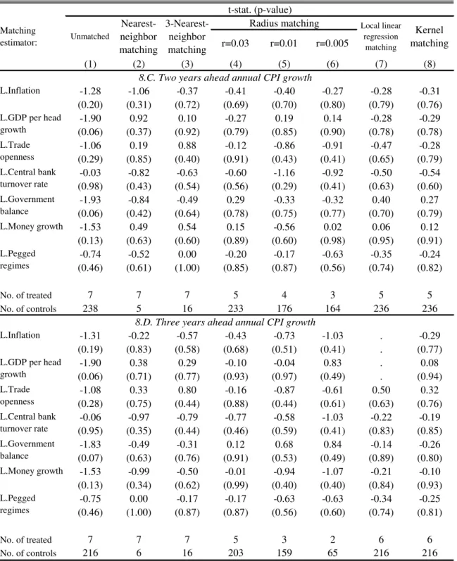
14 _{To check for the balancing of the covariates, in Appendix B, Table B, I present t-tests of differences}

insignificant. Government balance surplus becomes negative and significant, with the

non-intuitive implication that IT adopters have looser fiscal policies.15 A greater

difference, and with an important implication, is that sensitivity to per capita GDP growth

changes to negative and significant in most of the subsamples, meaning that countries

with weaker output growth are also more probable to adopt IT in the sample. Although

PSM protocols would suggest the exclusion of observables that do not influence IT

adoption or inflation, since my objective in this subsection is just to review LY’s results,

I keep all of them to the end. 16

As stated before, another criticism to LY is that in trying to make sense of the

short-run effects of monetary policy, there is an inflation-output tradeoff to be chosen by

the central banker. For ITers already on their inflation targets, or below the targets – and

such cases happened according to Johnson (2002) – the IT confidence bonus can translate

into loose demand policies and higher short-term output growth. With this perspective of

monetary policy tradeoffs, I present estimates of the IT policy effects for inflation and

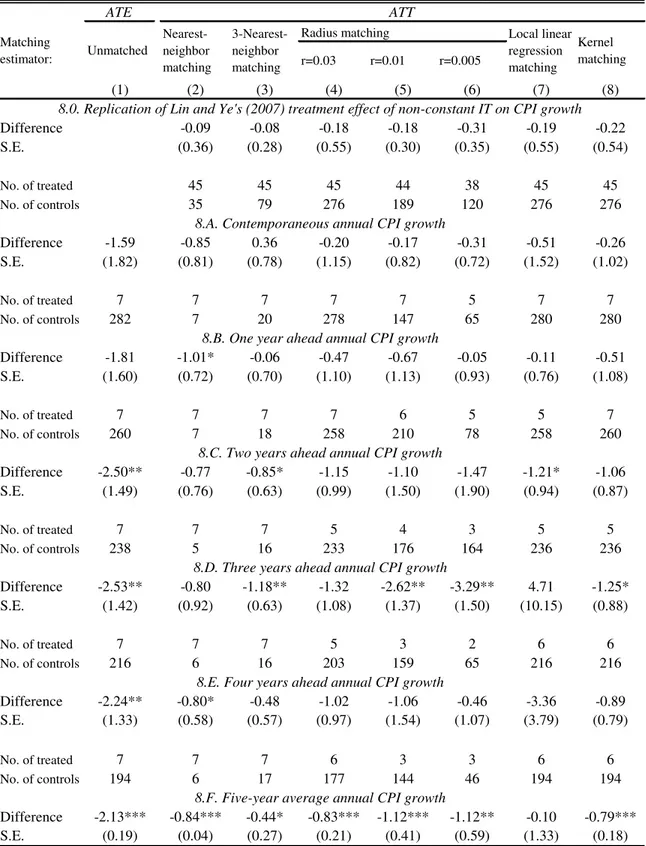
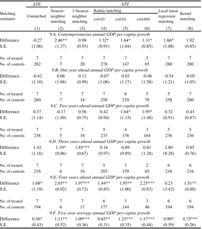
output growth in Tables 8 and 9. Panels A to E show the average treatment effect, ATEh

, in column (1), and the average treatment effect on treated, ATT_h , for h=0, 1, 2, 3, 4 in

columns (2)-(8), calculated according to equation (3). Panel 0 in Table 8 replicates LY’s

approach (also reproduced in Appendix C, Table C.2 for the referee’s benefit) and panel

F presents the five-year average ATE5 and ATT5 values, calculated according to

equation (4).

<Insert Tables 8 and 9 around here>

15 _{The negative coefficient for L.CGGDP is basically driven by Finland and Sweden, which ran central}

government deficits above 10% of the GDP in the year before their IT adoptions.

16 _{See also Vega and Winkelried (2005) and Mishkin and Schmidt-Hebbel (2002) for different propensity}

From Tables 8 and 9, in panels A to E, columns (2) to (8), the fact that the point

estimates of inflation and output growth differences are almost always favorable to ITers

against non-ITers is convincing. Overall, the ITers performed somewhat better than the

non-ITers in most of the cases, and significantly better in some cases. The ATTs for

inflation are negative in 33 out of 35 matches in Table 8, and the ATTs for output

growth are positive in 30 out of 35 matches in Table 9. If one looks at the five-year

average ATT5 , calculated from equation (4) in panels F, to infer the effects of monetary

policy on the inflation-output tradeoff, all inflation-output growth pairs of differences

have a negative-positive sign, respectively meaning that lower inflation was achieved

with higher growth. As in subsection 2.2, this is an unexpected result from the

perspective of an inexorable short-run positive inflation-output growth tradeoff, and

closer to Ball’s (1994a) credible disinflation. Except for the “local linear regression”,

ITers presented an average inflation around 1 percentage point lower and/or an average

output growth one percentage point higher in the first five-years of IT treatment, with

one, if not both, of the outcome differences significant at the 99% confidence level.

3. Conclusion

In a comprehensive survey on the empirical evidence on IT, Walsh (2009, p. 195)

concludes that “… macroeconomic experiences among both inflation targeting and

non-targeting developed economies have been similar,” a puzzling contrast with

policymakers’ enthusiasm for the system. If it is possible that recent IT adoptions by