Comparing the Performance of Ground Filtering Algorithms for Terrain Modeling in a Forest Environment Using Airborne LiDAR Data

ISSN 2179-8087 (online)

Original Article

Silviculture

Creative Commons License. All the contents of this journal, except where otherwise noted, is licensed under a Creative Commons Attribution License.

Comparing the Performance of Ground Filtering

Algorithms for Terrain Modeling in a Forest Environment

Using Airborne LiDAR Data

Carlos Alberto Silva

_{, Carine Klauberg}

_{, Ângela Maria Klein Hentz}

_,

Ana Paula Dalla Corte

_{, Uelison Ribeiro}

_{, Veraldo Liesenberg}

1_{Department of Natural Resources and Society, College of Natural Resources, University of Idaho – UI,} Moscow/ID, United States of America

2_{Rocky Mountain Research Station – RMRS, US Forest Service, Moscow/ID, United States of America} 3_{Department of Forest Science, Universidade Federal do Paraná – UFPR, Curitiba/PR, Brazil} 4_{Department of Silviculture, Universidade Federal Rural do Rio de Janeiro – UFRRJ, Seropédica/RJ, Brazil}

5_{Department of Forest Engineering, Universidade Estadual de Santa Catarina – UDESC, Lages/SC, Brazil}

ABSTRACT

The aim of this study was to evaluate the performance of four ground filtering algorithms to generate digital terrain models (DTMs) from airborne light detection and ranging (LiDAR) data. The study area is a forest environment located in Washington state, USA with distinct classes of land use and land cover (e.g., shrubland, grassland, bare soil, and three forest types according to tree density and silvicultural interventions: closed-canopy forest, intermediate-canopy forest, and open-canopy forest). The following four ground filtering algorithms were assessed: Weighted Linear Least Squares (WLS), Multi-scale Curvature Classification (MCC), Progressive Morphological Filter (PMF), and Progressive Triangulated Irregular Network (PTIN). The four algorithms performed well across the land cover, with the PMF yielding the least number of points classified as ground. Statistical differences between the pairs of DTMs were small, except for the PMF due to the highest errors. Because the forestry sector requires constant updating of topographical maps, open-source ground filtering algorithms, such as WLS and MCC, performed very well on planted forest environments. However, the performance of such filters should also be evaluated over complex native forest environments.

(Montealegre et al., 2015).

The Digital Terrain Model (DTM) derived from airborne LiDAR data is a representation of the bare surface, in other words, a surface free of any manmade and/or natural objects. DTMs are very useful for the delineation of watersheds and stream network extraction and are also a good source of data to perform geological and morphological analyses, as well as road planning (Sulaiman et al., 2010). However, the main challenge to obtain an accurate representation of a bare terrain is the efficiency of correctly classifying the ground returns out of the entire LiDAR dataset. According to Susaki (2012), the main errors that occur during the filtering of ground returns in a LiDAR dataset can be classified into two categories: i) type I or omission error, when the returns belonging to the ground are classified as other objects, such as vegetation or buildings; and (ii) type II or commission error, when small objects are erroneously classified as ground points. In addition, the accuracy of digital terrain modeling also depends on several other factors: a) sensor parameters and flight characteristics, such as the LiDAR pulse density (pulses∙m-2_{), which is}

a consequence of factors such as elevation and flight speed (Ruiz et al., 2014); b) characteristics of the land surface, such as topography and presence of dense and complex vegetation coverage (Sithole & Vosselman, 2004); and c) the processing techniques used to generate the DTM, such as the ground filtering algorithm and subsequently the interpolation method, as well as the spatial resolution of the DTM (Liu, 2008).

Currently, there are many algorithms available for filtering ground returns from airborne LiDAR data; some of them can be found in Montealegre et al. (2015), Julge et al. (2014), and Tinkham et al. (2011). The most well-known algorithms are those based on triangulated irregular networks - TIN (implemented in LAStools, Isenburg, 2015), weighted linear least squares - WLS (Kraus & Pfeifer, 1997, 1998), multi-scale curvature

cover commonly found in planted forest environments. Considering this theme, the main objective of this study was to evaluate the performance of four ground filtering algorithms used to generate DTMs.

2. MATERIAL AND METHODS

2.1. Study area

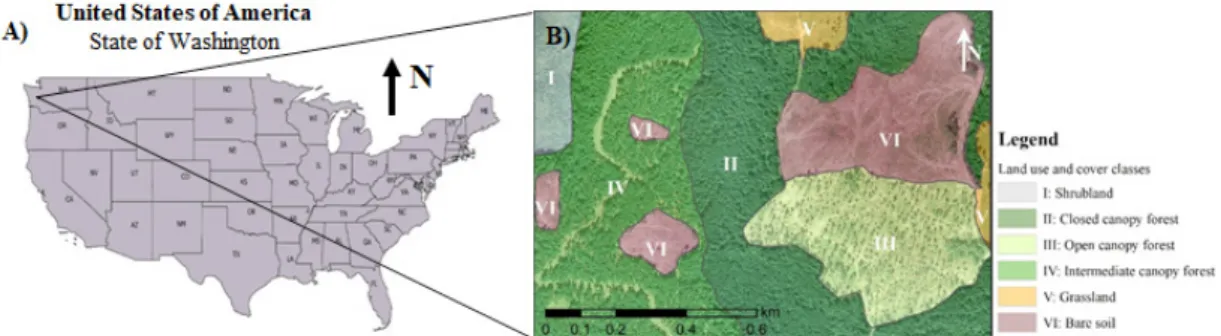
The study was conducted in a forest area belonging to Capitol State Forest located in western Washington state, USA. The study area covers approximately 122 hectares (Figure 1) and, according to Andersen et al. (2005), the forest is composed of species of conifers, such as douglas-fir (Pseudotsuga menziesii (Mirb.) Franco), western hemlock (Tsuga heterophylla (Raf.) Sarg.), and western red cedar (Thuja plicata Don.).

2.2. LiDAR data acquisition and processing

The LiDAR data are available at the Pacific Northwest Research Station (PNRS) portal of the US Forest Service (USFS). The LiDAR dataset is freely available for educational purposes. The LiDAR point cloud was downloaded from the official site of the LiDAR FUSION/LDV data processing and visualization program (McGaughey, 2015). The Saab TopEye system was shipped on a helicopter that flew over the entire study area (Figure 1). According to the data description, the LiDAR survey was performed in 1999 using a discrete feedback sensor. LiDAR data collection was performed with the following specifications: flying height of 200 m; flying speed of 25 m·s-1_{; swath width of}

70 m, forward tilt of ± 8 degrees; laser pulse density of 3.5 points·m-2_{; laser footprint of 40 cm, and laser pulse}

2.3. Land Use and Land Cover description

Concomitant with the LiDAR survey, aerial photographs were also acquired. These images were orthorectified by the USFS and resampled to spatial resolution of 30cm. Aiming to evaluate the performance of four ground filtering algorithms in different classes of land use and land cover, a visual classification was performed (Figure  1). The following classes were considered: Class I: Shrubland (4.72ha); Class II: Closed canopy forest (canopy cover ≥ 70%; 35.85ha); Class III: Open canopy forest (canopy cover ≤ 40%; 19.75ha); Class IV: Intermediate canopy forest (40% ≥ canopy cover ≤ 70%; 35.57ha); Class V: Grassland (3.89ha); and Class VI: Bare soil (21.93ha). Shrubland is a vegetation community characterized by shrubs, also including small sparse trees. The open, intermediate and closed canopy forest classes are related to tree density and canopy coverage after silvicultural interventions. Grassland is a class in which the vegetation is dominated by grasses rather than shrubs or small trees, although they may occur sparsely in some locations. Bare soil corresponds to areas with exposed terrain. In general, this class consists of areas in which clear cutting or harvesting of the trees occurs.

2.4. Ground filtering algorithms for the

filtering procedures and classifying ground

returns

Four different ground filtering algorithms were selected to generate DTMs. The four ground filtering algorithms used in this study are described ahead:

i)Weighted L inear L east Squares (WLS). The  WLS algorithm is available in GroundFilter

t o o l i m p l e m e n t e d i n F U S I O N / L D V.

The  FUSION  v.3.30  (McGaughey, 2015) is free software developed and maintained by the US Forest Service and used for LiDAR data processing and visualization. The WLS algorithm was first proposed by Kraus & Pfeifer (1997), and it combines both filtering and interpolation procedures. The chosen window size (cell size) for WLS was seven meters;

ii) Multi-scale Curvature Classification (MCC). The MCC algorithm is available in the MCC-LiDAR software. The MCC was also developed and maintained by the USFS. The MCC was first proposed by Evans & Hudak (2007), and it aims to generate DTMs from LiDAR data. The MCC algorithm operates through the elimination of points exceeding a given curvature threshold calculated over an interpolated surface known as spline (Evans & Hudak, 2007). Adjustment is performed with scale and curvature parameters. After testing several parameters, we chose the parameters of scale and curvature of 1.5 and 0.3, respectively;

algorithm selects the lowest points in each block in order to start the filtering procedure. After that, a triangulated irregular network (TIN) is built with these selected points. Next, an imaginary point is added to the point cloud, making a TIN densification. Finally, the TIN is progressively densified until all points are classified as ground or objects on this ground (Montealegre et al., 2015). In this study, the LASground tool was executed using a window size (step size) of 5m.

2.5. Generating and comparing digital terrain

models – DTMs

GridSufaceCreate, a tool implemented in FUSION/LDV, was used to create DTMs after the point cloud classification. This tool uses random points to create a grid surface on which the value of each cell is the mean elevation of all points within it (McGaughey, 2015). DTMs were generated with 1m resolution, compatible with the point density from the collected LiDAR data. The workflow to generate the DTMs is presented in Figure 2.

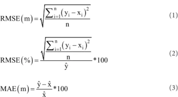
For comparison purposes, elevation values from 20,000 points randomly selected in the study area were extracted from the DTMs generated by each

( )

( )

n 2

i i i 1y x

n

RMSE % *100

ˆy

= −

=

∑

(2)

( ) y x MAE m ˆ ˆ 00

ˆ *1 x −

= (3)

where x_i is the elevation value from DTM 1, y_i is the elevation value from DTM 2, xˆ is the mean elevation from DTM 1, and yˆ is the mean elevation from DTM 2. The elevation values for each land cover class generated by the algorithms were also compared with each other by the Kolmogorov–Smirnov test using the ks.test function from the R software (R Development Core Team, 2016).

3. RESULTS AND DISCUSSION

The WLS, MCC, and PTIN ground filtering algorithms returned a similar classification of terrain points, whereas the PMF showed a distinct pattern in relation to the others (Figure 3). The PMF filtering generated a homogeneous density of points throughout the area, whereas the filtering output from the other algorithms resulted in regions with higher density of points on roads or open spaces and areas with lower

density of points, such as the regions of closed canopy forest. From the 4,859,996 original points, the WLS, MCC, PTIN and PMF algorithms classified as ground 1,910,755 (39.31%), 1,716,276 (35.31%), 1,327,550 (27.31%) and 121,071 (2.50%) points, respectively. The PMF algorithm classified a smaller number of points as ground than the other algorithms, corroborating the findings by Sulaiman et al. (2010).

The WLS and MCC filtered point clouds presented high density of points, mainly in the eastern region of the study area, where the classes of exposed soil and low density forest land use are predominant. In this

of 5%. Therefore, the differences between the DTMs are considered punctual.

Difference maps were generated by subtracting the different DTMs to highlight the similarities and divergences between the algorithms (Figure 5). The DTM generated by the PMF is the most distinct from the others, mainly in relation to those generated by the WLS and MCC algorithms. The differences in elevation between the DTMs generated by the PMF and the other algorithms are usually positive; this means that the PMF tended to underestimate the DTM elevation values. In contrast, the MCC algorithm presented results very similar to those of the WLS and PTIN algorithms, and the WLS presented only small differences compared with the PTIN. It is also possible to highlight that most differences between WLS and

MCC are negative. In other words, the MCC algorithm presents higher elevation values, contrasting with the results generated by the PMF.

Regarding the land use and land cover classes, greater difference was observed in the DTMs from class I (Shrubland), followed by classes V (Grassland), VI (Bare Soil), and III (Open canopy forest). We observed that the differences in DTMs vary between classes and algorithms, according to the results of RMSE and MAE (Table 1).

these differences, the smallest one occurred in relation to the PTIN algorithm.

The PMF algorithm tends to underestimate terrain elevation, as observed for the relation with the other DMTs. In addition, some authors have observed that one of the main problems of the PMF algorithm is that it assumes a constant slope on the area (Hui et al., 2016), a very difficult condition to be observed in forest environments, whether native forest or commercial plantations. The same assumption is valid for the study area, which presents flat regions in the center and abrupt inclinations in the outermost areas. We observed that

II – Closed-canopy

forest 5924

0.27 0.08 0.01

13° 14’ 7° 19’ WLS vs. PTIN 0.17 0.05 -0.01

WLS vs. PMF 0.23 0.07 -0.02 MCC vs. PTIN 0.26 0.08 -0.02 MCC vs. PMF 0.30 0.09 -0.02 PTIN vs. PMF 0.20 0.06 -0.01 WLS vs. MCC

III – Open-canopy

forest 3249

0.19 0.05 0.00

9° 24’ 5° 33’ WLS vs. PTIN 0.16 0.05 -0.01

WLS vs. PMF 0.22 0.06 -0.03 MCC vs. PTIN 0.18 0.05 -0.01 MCC vs. PMF 0.25 0.07 -0.03 PTIN vs. PMF 0.18 0.05 -0.02 WLS vs. MCC

IV – Intermediate

canopy forest 6508

0.19 0.05 0.00

12° 07’ 7° 27’ WLS vs. PTIN 0.16 0.05 -0.01

WLS vs. PMF 0.22 0.06 -0.03 MCC vs. PTIN 0.18 0.05 -0.01 MCC vs. PMF 0.25 0.07 -0.03 PTIN vs. PMF 0.18 0.05 -0.02 WLS vs. MCC

V - Grassland 613

0.13 0.04 0.00

16° 17’ 8° 06’ WLS vs. PTIN 0.16 0.05 -0.02

WLS vs. PMF 0.27 0.09 -0.06 MCC vs. PTIN 0.13 0.04 -0.02 MCC vs. PMF 0.28 0.09 -0.06 PTIN vs. PMF 0.25 0.08 -0.04 WLS vs. MCC

VI – Bare soil 3568

0.10 0.03 0.00

11° 23’ 6° 10’ WLS vs. PTIN 0.15 0.05 -0.02

WLS vs. PMF 0.25 0.08 -0.06 MCC vs. PTIN 0.12 0.04 -0.02 MCC vs. PMF 0.26 0.08 -0.06 PTIN vs. PMF 0.21 0.06 -0.04

N = number of observations; RMSE = Root mean square error; MAE = Mean absolute error; SD = Standard deviation.

first two land use and land cover classes, whereas for the other classes, the values were null. The differences between the other algorithms for all other classes were negative in all cases, which means that MCC and WLS estimate elevation values slightly higher than the other algorithms. Although there are variations between the DTMs, the results are very similar, with a maximum 0.06% MAE and; therefore, the algorithms present only punctual differences.

4. CONCLUSIONS AND

RECOMMENDATIONS

that the selected open-source algorithms, such as WLS and MCC, can be used to process airborne LiDAR data and provide accurate DTMs.

Despite the similarity between the four selected ground filtering algorithms, the PMF algorithm generated the most different results. This was due to underestimation of the DTM elevation, particularly in open canopy forest areas. The PMF algorithm tends to eliminate ground points excessively and, therefore, generates less consistent DTMs. In this study, regardless of the land use and land cover class, the greatest differences between the DTMs occurred in the areas with the highest slopes.

We suggest evaluating the potential of these algorithms in tropical native forest environments. Usually, the remaining forests are in areas with complex topography. We also suggest evaluation of the impact of algorithm selection in the estimation of individual tree heights for forest inventory purposes.

SUBMISSION STATUS

Received: 11 apr., 2016 Accepted: 8 apr., 2017

CORRESPONDENCE TO

Carlos Alberto Silva

Department of Natural Resources and Society, College of Natural Resources, University of Idaho – UI 875 Perimeter Drive 83843, Moscow, I ID, United States of America

e-mail: carlos_engflorestal@outlook.com

REFERENCES

Andersen H-E, McGaughey RJ, Reutebuch SE. Forest measurement and monitoring using high-resolution airborne LiDAR. In: Harrington CA, Schoenholtz SH, editors. Productivity of western forests: a forest products

focus. Portland: USDA/Forest Service; 2005.

Axelsson P. DEM generation from laser scanner data using adaptive TIN models. International Archives of

Photogrammetry and Remote Sensing 2000; 33(B4/1):

110-117.

Carter J, Schmid K, Waters K, Betzhold L, Hardley B, Mataosky R et al. Lidar 101: an introduction to LiDAR Technology, Data, and Applications. Charleston: National Oceanic and Atmospheric Administration (NOAA) Costal Services Center; 2012; 76 p.

Evans JS, Hudak AT. A multiscale curvature algorithm for classifying discrete return LiDAR in forested environments.

IEEE Transactions on Geoscience and Remote Sensing

2007; 45(4): 1029-1038. http://dx.doi.org/10.1109/ TGRS.2006.890412.

Hui Z, Hu Y, Yevenyo YZ, Yu X. An improved FMPological algorithm for filtering airborne LiDAR point cloud based on multi-level kriging interpolation. Remote Sensing

2016; 8(35): 1-16.

Isenburg M. LAStools – efficient tools for LiDAR processing, version 150304. 2015 [cited 2016 Jan 5]. Available from: http://lastools.org

Julge K, Ellmann A, Gruno A. Performance analysis of freeware filtering algorithms for determining ground surface from airborne laser scanning data. Journal of Applied Remote Sensing 2014; 8(1): 083573-1, 083573-15. http://dx.doi.org/10.1117/1.JRS.8.083573.

Kraus K, Pfeifer N. A new method for surface reconstruction from laser scanner data. International

Archives of Photogrammetry and Remote Sensing 1997;

32(3/2W4): 80-86.

Kraus K, Pfeifer N. Determination of terrain models in wooded areas with airborne laser scanner data. ISPRS Journal of Photogrammetry and Remote Sensing 1998; 53(4): 193-203. http://dx.doi.org/10.1016/S0924-2716(98)00009-4. Liu X. Airborne LiDAR for DEM generation: some critical issues. Progress in Physical Geography 2008; 32(1): 31-49. http://dx.doi.org/10.1177/0309133308089496.

McGaughey RJ. FUSION/LDV: software for LIDAR data analysis and visualization.  v.3.3. Washington: USDA/ Forest Service; 2015.

Montealegre AL, Lamelas MT, Riva J. A comparison of open-source LiDAR filtering algorithms in a Mediterranean forest environment. IEEE Journal of Selected Topics in Applied Earth Observations and Remote Sensing 2015; 8(8): 4072-4085. http://dx.doi.org/10.1109/JSTARS.2015.2436974. R Development Core Team. R: A language and environment for statistical computing. Vienna, Austria: R Foundation for Statistical Computing; 2016 [cited 2016 Jan 10]. Available from: http://www.R-project.org

Ruiz LA, Hermosilla T, Mauro F, Godino M. Analysis of the influence of plot size and LiDAR density on forest structure attribute estimates. Forests 2014; 5(5): 936-951. http://dx.doi.org/10.3390/f5050936.

Sithole G, Vosselman G. Experimental comparison of filter algorithms for bare-Earth extraction from airborne laser scanning point clouds. ISPRS Journal of Photogrammetry and Remote Sensing 2004; 59(1-2): 85-101. http://dx.doi. org/10.1016/j.isprsjprs.2004.05.004.