Channel Estimation using Adaptive Filtering for
LTE-Advanced
Saqib Saleem1, Qamar-ul-Islam
Department of Communication System Engineering Institute of Space Technology
Islamabad, Pakistan
Abstract
For demand of high data rates, enhanced system capacity and coverage, ITU made proposal for the standardization of next generation wireless communication systems, known as IMT-Advanced. To achieve these targets, a priori knowledge of the channel is required at the transmitter side. In this paper, three adaptive channel estimation techniques: Least Mean Square (LMS), Recursive Least Square (RLS) and Kalman-Filtering Based, are compared in terms of performance and complexity. For performance, Mean Square Error (MSE) and Symbol Error Rate (SER) while for complexity, computational time is measured for variable channel impulse response (CIR) lengths and channel taps. MATLAB Monte-Carlo Simulations are used to evaluate these techniques.
Keywords: LTE-A, Kalman Filtering, LMS, LSE, RLS,
LMMSE, DFT-based, DCT-Based, Windowed DFT-Based
1. Introduction
3GPP’s proposed LTE-A system is aimed at fulfilling the requirements of IMT-Advanced [1]. To meet the specification made by IMT-A, the following enhancements are proposed for LTE-A, in Release-10: Support for wider bandwidth, Co-ordinated multi-point transmission and reception (CoMP), relaying, support for Self-Organizing Networks (SON) and mobility enhancements of Home enhanced-Node-B (HeNB) etc [2].
A hybrid form of OFDMA and SC-FDMA is used for OFDM system implementation at radio bearer of LTE-Advanced. The minimum proposed sector throughput in Release-10 is 1.2 for UL and 2.4 for DL and maximum cell-edge throughput is 0.07 for , UL and 0.12 for , and DL .The peak data rate requirement of 1Gbps, as proposed in IMT-Advanced, can be achieved in LTE-A using MIMO and wider transmission bandwidth of 70 MHz which can be achieved through carrier aggregation [3].The peak spectral efficiency of 30 bps/Hz for DL and 15 bps/Hz for UL can be achieved by using beam-forming and Multi-User MIMO techniques. The channel can be made known at the transmitter by either sounding reference signals, user specific demodulation reference signals (DM-RS) or cell-specific reference signals. For reliable communication in attenuated time-dispersive multi-path fading channels adaptive modulation and coding (AMC) technique with
adaptive equalization has been proposed in [4]. For these adaptive techniques, used in 4G wireless communication systems, iterative receivers employing joint detection and decoding are proposed in [5]. The channel can also estimated by using adaptive filtering techniques such as RLS, LMS [6]. We can make use of second order channel and noise statistics for these algorithms. The state of the art channel estimation techniques such as LSE and LMMSE are optimized in [7] and [8]. While in [9] and [10], the transform based channel estimation techniques such as DFT-based, DCT-based and Windowed DFT-based are discussed. In this paper the performance and complexity evaluation of RLS, LMS and well-known Kalman-Filtering channel estimation algorithms are carried out based on the different channel length and multipath channel taps, while depending on the second order channel and noise statistics
In Section II, system description according to Rel-10 of LTE-A is given and proposed channel estimation algorithms are explained in Section III with their simulation results discussed in Section IV and conclusions are drawn in Section V.
2. System Description
2.1
Frame Structure for LTE-A
In LTE-A, according to Rel-10, Generic radio frame is used for TDD and FDD while alternative radio frame is transmitted only for TDD mode. First one contains 20 sub-frames, each of length and second radio frame can be divided into 2 sub-frames, each of same length as for the first one sub-frame. The number of sub-carriers used for OFDM for each sub-frame are
[1]. The number of OFDM symbols per sub-frame can be 6 or 7 for Generic frame and for alternative frame can be 8 or 9.
For channel estimation, the 2-Dimensional transmitted DL reference signals from each antenna are given by the following relation [2]
, , ,
Where , shows 2-dimensional orthogonal sequence and
structure is shown in Figure 1.
Fig. 1 Mapping of Reference Signals for Generic Frame Structure [2]
According to Rel-9, these reference signals can be used either for PDSCH demodulation or for channel estimation, for which these reference signals can be made cell-specific and can be transmitted as the data sequence.
2.2 System Model
The transmitting OFDM signal over the Rayleigh fading channel can be generated by
Where . is the OFDM Symbol time and is the cyclic prefix length for sub-carrier, which can be 144,160 or 512 for Generic frame and 224 or 512 for alternative radio frame.
The necessary steps carried out in an OFDM system are shown in Figure.2.In OFDM, a signal of wider bandwidth is divided in smaller bandwidth signals to have flat fading effect to avoid Inter-Symbol Interference (ISI). Then IFFT is applied to these sub-carriers and CP is added to each sub-carrier to avoid ICI. After receiving the signal, before applying FFT operation, first CP is removed and then we have the following received symbols over sub-carrier [11]
Where is ICI component occurring between different sub-carriers, occurring in high mobility situations, and is given by [11]
For a wireless channel having multipaths.
shows zero mean AWGN noise with variance for sub-carrier.
The channel impulse response (CIR) of the wireless channel is given by [11]
,
where is the multipath gain having Rayleigh Distribution and is given by [10]
| |
denotes the corresponding multipath delay and is the power delay constant.
Channel Frequency Response (CFR) for Eq.5 can be written as [11]
, ∆
∆ is the sub-carrier’s spacing to avoid ICI.
3. Channel Estimation
3.1 RLS Channel Estimation
At each iteration, the transmitted data sequence and the desired output sequence is required to make LSE as adaptive channel estimation technique, which is not possible to get in real-time processing. In RLS algorithm, we need only new data values at each iteration and it is based on initially LSE estimated co-efficients at iteration [6].
At iteration , we require to minimize the following function
,
Where , is the weighting factor, having the following exponential form
,
Where should be close to 1.
In RLS channel estimation following steps are carried out
1- The up-dation of correlation matrix is given by
2- Adaptation gain becomes
3- The value of a priori error is
4- The conversion factor at iteration
5- The updated value of co-efficients becomes
The estimated channel after iteration becomes
Where is RLS filter length.
The value of gain vector at iteration is given by
And
At start of RLS algorithm, the initialization parameters are taken as
.
where
.
3.2 LMS Channel Estimation
For less complex LSE and LMMSE [7] requiring no matrix inversion, LMS algorithm is proposed for the solution of Wiener-Holf equation, for which statistical information of the channel and data may be required for better performance. The necessary steps carried out in LMS channel estimation are given below
1- Initially the channel is estimated by using LSE technique, giving .
2- After finding the co-efficients, the estimation of the channel becomes
Where
…
Where is LMS filter length.
3- Error at iteration is given by
4- Co-efficient are updated according to
Where is the adjustable step-size parameter.
5- Error given by weight vector is
Mean Square Error (MSE) given by the LMS algorithm is defined as
Where
. shows the expectation operator.
For real-time wireless communication, the value of the step-size parameter is taken very small. In order to make LMS algorithm more stable, the optimal value of adaptation constant is given by
,
Where
Where denotes doppler spread of channel tap, P is total number of reference signals used in radio frame and
is the operating SNR value.
For slow co-efficient updating with better performance
is used but for less computational time is used, giving .
3.3 Leaky-LMS Channel Estimation
In order to avoid the unstabilization of the LMS algorithm under no convergence conditions, a leakage co-efficient is used in conventional LMS which gives the following co-efficient up-dation relation [13]
Where .
3.4 Normalized LMS Channel Estimation
For minimum disturbance and fast convergence, NLMS technique is proposed [13]
Where is a small-value constant. This algorithm is equivalent to time-varying step-size LMS algorithms, showing fast convergence rate than conventional LMS.
3.5
LMS Channel Estimation
function can also be used in LMS to make hardware implementation less costly and is given by [13]
3.6 Linearly Constrained LMS Channel Estimation
For better performance, some channel constraints can be taken into account, resulting in the following adaptation rule [13]
′
Where
′
3.7 Self-Correcting LMS Channel Estimation
In this approach the estimated channel is compared with the ideal channel to make channel estimation. At iteration , the estimation is channel is given by[13]
3.8 Kalman-Filtering based Channel Estimation
According to [14], the channel estimation problem can be formulated by the following state space vector
Where … , is channel matrix showing the state transition of and
is the complex white Gaussian noise. The received signal is represented by [15]
Considering the noise and the channel statistics, the following recursive Kalman-Filtering equations are performed for channel estimation [16].
/ /
/ /
,
/
/
/ / / (40)
/ /
The parameters at initialization are
/ /
is the Kalman filter gain.
is the covariance matrix of the noise .
/ / /
(44)
4. Simulation Results
Monte-Carlo Simulations for QPSK modulation for a generic radio frame having CAZAC sequence as reference signals are performed for a bandwidth of 70 MHz and carrier frequency of 2 GHz. FFT size is 2048 and Jake’s model over 64-tap Rayleigh fading channel described by EVA power delay profile, is simulated.
Table 1: Comparison of LS, LMS and RLS 5000 Simulations
(mSec)
1 OFDM Symbol
(nSec)
1 Bit (nSec)
LS 0.34 5.24 2.62
LMS 1.9 29.68 14.84
RLS 1.8 28.12 14.06
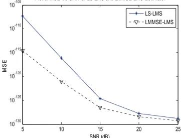
For LMS technique, initially the channel can be estimated by LS or LMMSE approach. The performance comparison of these two approaches is shown in Figure 3. There is a difference in performance at low SNR values and LMMSE-LMS is preferred but it results in more complexity as it depends on the channel statistics. But as we go increasing the SNR value, both techniques show same performance behavior. So for high SNR conditions LSE-LMS is proposed as it has less complexity than LMMSE-LMS. The computational time of LMS and RLS as compared to simple LSE is given in Table 1. LMS has almost 6% more complexity than RLS and both LMS and RLS have approximate 400 % more computation time than LSE. The complexity of different variants of LMS is given in Table 2.
Fig. 3 MSE v/s SNR for LS-LMS and LMMSE-LMS Estimators
5 10 15 20 25
10-130
10-125
10-120
10-115
10-110
10-105
SNR (dB)
MS
E
Plot of MSE v/s SNR for LS-LMS and LMMSE-LMS Estimator
Table 2: Computational Time for different LMS Algorithms =0.1
(mSec)
=0.5 (mSec)
=0.9 (mSec)
LMS 9.8 9.7 9.6
Leaky-LMS 10.5 9.8 9.6
-LMS 10.5 9.8 9.8
NLMS 19.1 19.2 19.2
Norm-sign-LMS 19 19 19.1
Constrained-LMS 13.2 13.2 13.2
Self-correcting LMS 11.3 10.2 10.1
Normalized-LMS and Norm-sign-LMS have more complexity than all others approaches. The effect of varying the step-size parameter is more prominent for Leaky-LMS, where for 400% increment of step-size results only in 7% reduction in complexity. The step-size value does not change the complexity in case of Norm-sign-LMS and constrained-LMS.
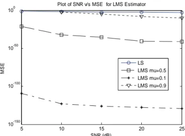
The effect of step-size values on MSE for LMS channel estimation is given in Figure 4. For any value of step-size, LMS performs better than LSE. By increasing step-size from 0.1 to 0.5, the performance degrades significalty but furhter increment of step-size does not have soo much impact on performance. The performance of LMS for different values of step-sizes in terms of Symbol Error Rate (SER) is shown in Figure 5. Here again performance is better for small values of step-size and increment in value of step-size degrades the performance for all SNR values.
Fig. 4 MSE v/s SNR for LMS for different Step-Size Values
Fig. 5 SER v/s SNR for LMS for different Step-Size values
Fig. 6 MSE v/s SNR for LMS for different Channel Taps
The performance for different channel taps for LMS is given in Figure 6. By decreasing the channel taps from 20 to 10, there is a significant effect on performance but further reduction on number of channel taps does not degrade the performance too much, especially at low SNR the performance remains same and advantage comes in form of reduced complexity.
The performance for different Leakage Co-efficients for Leaky-LMS is demonstrated in Figure 7. We come to know that by increasing the leakage co-efficient values, the performance degrades, especially at low SNR values but this change in value of leakage co-efficient does not effect performance at high SNR values.
5 10 15 20 25
10-150 10-100 10-50 100
SNR (dB)
MSE
Plot of SNR v/s MSE for LMS Estimator
LS LMS mu=0.5 LMS mu=0.1 LMS mu=0.9
5 10 15 20 25 30
0.46 0.47 0.48 0.49 0.5 0.51 0.52
SNR (dB)
S
y
m
b
o
l E
rro
r R
a
te
Plot of SER vs SNR of LMS Estimator for different mu
mu=0.5 mu=0.1 mu=0.9
5 10 15 20 25
10-170
10-160
10-150
10-140
10-130
10-120
10-110
SNR (dB)
MS
E
MSE v/s SNR for different Channel Taps for LMS Estimator
Fig. 7 MSE v/s SNR for Leaky-LMS for different Leakage Co-efficients
The performance of NLMS improves by increasing the value of from 0.15 to 1. This improvement is seen only at low SNR values as shown in Figure 8. But by increasing this value further to 2 the performance degrades for all SNR values so this constant term is normally preferred less than 1.
Fig. 8 MSE v/s SNR for NLMS for different values of
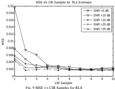
Fig. 9 MSE v/s CIR Samples for RLS
The performance for different Channel impulse response samples for RLS is shown Figure 9 for different SNR operating conditions.CIR samples more than 5 or 6 does not improve performance and only results in increased complexity. But for CIR samples less than 5, the performance goes on improving as SNR value is increased. The effect of channel taps on performance of RLS is also given in Figure 10. Here we observe that for all SNR values we have same performance. Performance improves up-to 10 channel taps after that only complexity increases and there is no effect on performance.
Fig. 10 MSE v/s Channel Taps for RLS Estimator
10 12 14 16 18 20 22 24
10105
10110
10115
SNR (dB)
MS
E
Plot of MSE vs SNR of Leaky-LMS Estimator for different Leakage Co-efficient
Leakge Coefficient=0.1 Leakge Coefficient=0.9 Leakge Coefficient=0.5
6 8 10 12 14 16 18 20 22 24
10-5
SNR (dB)
MS
E
Plot of MSE vs SNR of NLMS for different Constant Term Values
Constant Term=1 Constant Term=0.5 Constant Term=0.15 Constant Term=2
1 2 3 4 5 6 7 8 9 10
0 0.002 0.004 0.006 0.008 0.01 0.012 0.014 0.016 0.018 0.02
MSE v/s CIR Samples for RLS Estimator
CIR Samples
MS
E
SNR =5 dB SNR =10 dB SNR =15 dB SNR =20 dB SNR =25 dB
0 10 20 30 40 50 60 70
0.01 0.02 0.03 0.04 0.05 0.06 0.07 0.08
MSE v/s Channel Taps for RLS Estimator
Channel Taps
MSE
Fig. 11 MSE vs SNR for LMS, RLS and Kalman-Based CE
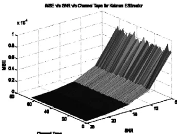
A comparison of Kalman-Based channel estimation with RLS and LMS is shown in Figure 11. Kalman Filtering shows better performance than both RLS and LMS at all SNR values. Its performance is significantly better than LMS as compared to RLS. The MSE vs Channel Taps is given in Figure 12. For all channel taps, high value of SNR is preferred. And we also observe that for a specific SNR value, there is no effect of changing the number of channel taps on the performance and we have to only pay for more complexity. That is why for Kalman channel estimation, less number of channel taps are preferred. The combined effect of channel taps and SNR on performance is given in Figure 13.
The performance of Kalman-Based channel estimation technique for different values of CIR samples is shown in Figure 14. The performance remains same for CIR samples more than 4 but at the cost of more complexity. For high SNR values, different values of CIR samples does not affect the performance so for high SNR operating conditions we prefer less number of CIR samples to be considered. The effect of CIR Samples and SNR on MSE for Kalman Filtering is given in Figure 15.
Fig. 12 MSE vs Channel Taps for Kalman Filtering
Fig. 13 MSE vs SNR vs Channel Taps for Kalman Filtering
Fig. 14 MSE vs CIR Samples for Kalman Filtering
Fig. 15 MSE vs SNR vs CIR Samples for Kalman Filtering
5 10 15 20 25
10-4 10-3 10-2 10
SNR (dB)
MSE
Kalman Filtering LMS RLS
0 10 20 30 40 50 60 70
0 0.1 0.2 0.3 0.4 0.5 0.6 0.7 0.8 0.9
1x 10
-4
MSE v/s Channel Taps for Kalman Estimator
Channel Taps
MSE
SNR =5 dB SNR =10 dB SNR =15 dB SNR =20 dB SNR =25 dB
1 1.5 2 2.5 3 3.5 4 4.5 5
0 0.01 0.02 0.03 0.04 0.05 0.06 0.07
MSE v/s CIR Samples for Kalman-based CE
CIR Samples
MS
E
SNR =5 dB SNR =10 dB
SNR =15 dB SNR =20 dB
5. Conclusion
In this paper, three adaptive channel estimation algorithms, RLS, LMS and Kalman-Filtering based, are compared in terms of performance, MSE and SER, and complexity. The performance is measured for different filter lengths and multipath channel taps. Leaky-LMS shows better performance among all LMS techniques with less computation time. Kalman-Filtering shows better performance as compared to both LMS and RLS. For optimized channel estimator employing Kalman Filtering in wireless communication system, 4-5 CIR samples and any number of channel taps can be used. But for less complexity, channel taps should be less than 10.
References
[1] 3GPP TS 36.211 v.8.5.0, “Physical Channels and Modulation”, 2008
[2] 3GPP TS 36.814 v.9.0.0, “Further Advancements for E-UTRA Physical Layer Aspects”, 2009 [3] 3GPP Release 10 v.0.0.6, “Overview of Release
10”, 2010
[4] Lars Lindbom,”Simplified Kalman Estimation of Fading Mobile Radio Channels: High Performance at LMS Computational Load”,
0-7803-0946-4, IEEE 1993
[5] Jongsoo Choi, Martin Bouchard and Ter Hin Yeap,”Adaptive Filtering-Based Iterative Channel Estimation for MIMO Wireless Communication”,
0-7803-8834-8, IEEE 2005
[6] Saqib Saleem, Qamar-ul-Islam, ” LMS and RLS Channel Estimation Algorithms for LTE-Advanced”, Journal of Computing Vol. 3
Issue.04, pp-155-163, April 2011
[7] Saqib Saleem, Qamar-ul-Islam, ” Optimization of LSE and LMMSE Channel Estimation Algorithms based on CIR Samples and Channel Taps”, IJCSI
International Journal of Computer Science Issues Vol. 8 Issue.01,pp-437-443,January 2011
[8] Saqib Saleem, Qamar-ul-Islam, ” Performance and Complexity Comparison of Channel Estimation Algorithms for OFDM System”,
IJECS International Journal of Electrical and Computer Sciences , Vol. 11, No.02,pp-6-12,April 2011
[9] Saqib Saleem, Qamar-ul-Islam, ” On Comparison of DFT-based and DCT-based Channel Estimation for OFDM System ”, Accepted for publication in IJCSI International Journal of
Computer Science Issues Vol. 8 Issue.03,May 2011
[10] Saqib Saleem, Qamar-ul-Islam, ” Transform-Based Channel Estimation Techniques for
LTE-Advanced”, Journal of Computing Vol. 3
Issue.04, pp-164-169, April 2011
[11] Yongming Liang, Hanwen Luo, Jianguo Huan,”Adaptive RLS Channel Estimation in MIMO OFDM Systems”, 0-7803-9538, IEEE
2005
[12] Soeg Geun Kang, Min Ha and Eon Kyeong Joo, “A comparative Investigation on Channel Estimation Algorithms for OFDM in Mobile Communication”, IEEE Transactions on Broadcasting, Vol. 49, No. 2, June 2003.
[13] Alexandar D.Poularikas, “Adaptive Filtering
Primer with MATLAB” Taylor & Francis.
[14] Valery Ramon, Cedric Herzet, Xavier Wautelet and Luc vandendrope,”Soft Estimation of time-varying frequency selective channels using Kalman smoothing”, IEEE ,1-4244-0353-7
[15] Hala mahmoud, Allam Mousa, Rashid Saleem, “ Kalman Filter Channel Estimation Based on Comb-Type Pilots for OFDM System in Time and Frequency-Selective Fading Environments”, IEEE
MIC-CCA 2008
![Fig. 1 Mapping of Reference Signals for Generic Frame Structure [2]](https://thumb-eu.123doks.com/thumbv2/123dok_br/16364748.190545/2.918.84.439.162.445/fig-mapping-reference-signals-generic-frame-structure.webp)