STABILIZABILITY OF NONMINIMUM PHASE UNSTABLE PLANTS WITH
ARBITRARY MULTIPLICITY OVER AWGN CHANNELS
Alejandro J. ROJAS
∗ [email protected]∗Departamento de Ingeniería Eléctrica Universidad de Concepción
Concepción, Chile
RESUMO
Estabilizabilidade de plantas instáveis de fase não mí-nima com multiplicidade arbitrária através de canais AWGN
Neste artigo, obtemos a relação sinal-ruído ínfimo (SNR) necessário para a estabilizabilidade de um laço linear saída de realimentação ao longo de um canal de Gaussian aditivo branco ruído (AWGN) em forma fechada. O foco em canais AWGN nos permitirá, então, definir a capacidade do canal mínima exigida para estabilizabilidade. Finalmente, o SNR ínfimo para estabilizabilidade também nos permitem identi-ficar em closed-formar o relacionado estabilização solução positiva Hermitiana semidefinida para a equação de Riccati de tempo contínuo algébrica de controle LQ com desaparecer o peso do Estado e autovalores repetidos.
PALAVRAS-CHAVE: Controle sobre redes; sinal-ruído
ín-fimo; Canal de ruído gaussiano aditivo branco ; pólos instá-veis repetidos ; zeros de fase não minimos repetidos; Tempo de atraso; capacidade de canal; equação algébrica de Riccati contínua no tempo
.
ABSTRACT
In the present paper we obtain the infimal signal-to-noise ratio (SNR) required for the stabilizability of a linear
out-Artigo submetido em 11/01/2011 (Id.: 1247) Revisado em 05/05/2011, 05/11/2011, 01/12/2011
Aceito sob recomendação do Editor Associado Prof. Daniel Coutinho
put feedback loop over an additive white Gaussian noise (AWGN) channel in closed-form. The focus on AWGN channels allow us to then define the minimal channel capac-ity required for stabilizabilcapac-ity. Finally, the infimal SNR for stabilizability also allow us to identify in closed-form the re-lated stabilizing Hermitian positive semidefinite solution to the continuous-time algebraic Riccati equation of LQ control with vanishing state weight and repeated eigenvalues.
KEYWORDS: Control over networks; Infimal signal-to noise
ratio; Additive white Gaussian noise channel; Repeated un-stable poles; Repeated nonminimum phase zeros; Time de-lay; Channel capacity; Continuous-time algebraic Riccati equation.
1
INTRODUCTION
The main objective of control design is to direct the output of a system to a given desired target. It is well known that if the system, or plant model, is stable then a simple open loop configuration can potentially suffice. However, in practice, the use of feedback control is advised since it allow us to reject disturbances, deal with plant model uncertainties, and to include the case of unstable plant models.
linear time invariant (LTI) case it is thus well understood that the cause of such limitations resides on the presence and in-teraction of unstable poles, nonminimum phase (NMP) zeros and time-delay (see for example (Seron et al., 1997) and ref-erences therein).
In the last decade, the study of fundamental limitations has been extended to design problems of control over commu-nication networks. The authors of (Braslavsky et al., 2007) and (Braslavsky et al., 2005) obtained the expression for the infimal SNR required to stabilize a finite dimensional un-stable LTI plant over a memoryless additive white Gaus-sian noise (AWGN) channel when considering unstable plant poles, NMP zeros and plant time-delay. On the other hand, the additive colored Gaussian noise channel with memory has been studied for example in (Rojas, 2011), whilst perfor-mance limitations have also been considered for example in (Rojas, 2009c), (Silva et al., 2010) and (Wang et al., 2011). Here, motivated by the potential insights that can be gained, we retake the AWGN channel approach focusing on output feedback stabilizability of plant models with repeated NMP zeros.
Our first contribution in this paper is to present the infimal SNR required for output feedback stabilizability of a plant with time delay, repeated unstable poles and NMP zeros over an AWGN channel. This result differs from (Rojas, 2009b, Theorem 4) in that we explicitly solve the Laplace variable derivative left stated in (Rojas, 2009b). This simple fact al-low us to investigate in more depth the implications stem-ming from the closed-form infimal SNR solution as shown by our other results reported here. Our second contribution, based on the known fact that the capacity of an AWGN chan-nel does not increase with feedback, is to restate the infimal SNR result into a necessary and sufficient condition on the channel capacity.
Riccati equations (Lancaster e Rodman, 1995; Abou-Kandil et al., 2003), in particular algebraic Riccati equations (AREs), are a recurrent and important feature in many the-oretical control design results, (Goodwin et al., 2001). The infimal SNR problem, here solved in closed-form, can also be addressed numerically as an LQ control problem by solv-ing a continuous-time algebraic Riccati equation with van-ishing state weight, see for example (Rojas, 2009a). It is then perhaps not entirely surprising that our third contribution, based on the equivalence of the infimal SNR result developed here with the result presented in (Braslavsky et al., 2005), is a closed-form characterization of the stabilizing Hermitian positive semidefinite solution to the continuous-time alge-braic Riccati equation with vanishing state weight that lays behind the infimal SNR problem. To the best knowledge of the author such closed-form solution is novel and differs
from (Rojas, 2010a) in that repeated unstable poles are ex-plicitly considered.
The paper is organized as follows: In Section 2 we introduce the assumptions for the present work. In Section 3 we present the infimal SNR for stabilizability result. In Section 4 we discuss the implications in terms of the channel capacity and connect the infimal SNR for stabilizability result to the sta-bilizing Hermitian positive semidefinite solution in closed-form of a related class of continuous-time algebraic Riccati equations with vanishing state weight. Finally, in Section 5, we give concluding remarks for the present work. A prelimi-nary version of the present results has been communicated in (Rojas, 2010d).
Terminology: letCdenote the complex plane. LetC−,C¯−, C+andC¯+ denote respectively the open left-plane, closed left-plane, open right-plane and closed right-plane ofC. Let Rdenote the set of real numbers,R+the set of positive real numbers,R+
o the set of non-negative real numbers andR
− the set of real negative numbers. Let Z+ denote the set of positive integers. A continuous-time signal is denoted byx(t), and its Laplace transform byX(s),s ∈ C. The expectation operator is denoted by E. A rational transfer function of a continuous-time system is minimum phase if all its zeros lie inC¯−, and is nonminimum phase if it has zeros in C+. The RH
∞ space consists of all proper and real rational stable transfer functions. The norm of a system
P(s)inH∞is given by ∥P∥∞ = supω∈R|P(jω)|, where
j=√−1. DefineL2as the space of functionsf :jR→C such that∥f∥2
2 = 21π
∫∞
−∞|f(jω)|
2dω < ∞. DefineH2
as the space of functionsf : C+ → Csuch that ∥f∥2 2 =
supσ>021π
∫∞
−∞|f(σ+jω)|
2dω <
∞. TheH2 space is a
(closed) subspace ofL2with functionsf(s)analytic inC+. Finally define alsoH⊥
2 as the space of functionsf :C−→C
such that∥f∥2
2= supσ<021π
∫∞
−∞|f(σ+jω)|
2dω <∞. The
H⊥
2 space is the orthogonal complement ofH2inL2, that is
the (closed) subspace of functions inL2that are analytic in
C−.
2
PRELIMINARIES
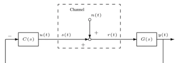
The assumptions for the closed loop system shown in Fig-ure 1 are for the continuous-time plant with time-delay to be defined as
G(s) =Go(s)e−sτ,
whereGo(s)is a nonminimum phase, rational transfer
func-tion with relative degreeng ≥1, containingmdistinct
un-stable polespi ∈ C+, i = 1,· · ·, meach with multiplicity
ni andqdistinct NMP zeros ζj ∈ C+, j = 1,· · · , q each
with multiplicityoj, also distinct of each and every
can be alternatively represented by a state-space description (A,B,C,0)that satisfies:
(1) (A, B, C, 0)is a minimal realization ofGo(s)such
that
A=
[
Au 0
0 As
]
, B=
[
Bu
Bs
]
, C=[Cu Cs
]
,
(1) whereA ∈ Cn×n, B ∈ Rn×1, C ∈ R1×n, Au ∈
Cnu×nu with n
u = ∑mi=1ni, Bu ∈ Rnu×1, Cu ∈
R1×nu.
(2) The eigenvalues ofAuare all inC+.
(3) Auis block-diagonal,
Au= diag{Ai},∀i= 1,· · ·, m,
with
Ai =
pi 1 0 · · · 0 0
0 pi 1 · · · 0 0
0 0 pi · · · 0 0
..
. ... ... ... ... ... 0 0 0 · · · pi 1
0 0 0 · · · 0 pi
∈Cni×ni,
andBu =
B1
.. .
Bm
withBTi = [0| {z }· · ·1 ni
]T for alli =
1,· · ·, m.
(4) The eigenvalues ofAsare all inC−.
Assumption (1) implies that the pair (Au, Bu)is
control-lable, (Kailath, 1980). Also notice that, in order to sat-isfy Assumption (3) forAu, we are implicitly assuming for
any original real coefficients system to be transformed into the equivalent system with A diagonal, (potentially)
con-taining complex conjugate coefficients. This can always be achieved by means of the transformation matrix collecting all the eigenvectors as explained in, for example, (Strang, 1988). As depicted in Figure 1 the channel model is a memoryless AWGN channel with the additive noise processn(t)assumed to be an i.i.d. zero-mean Gaussian white noise process with power spectral densityΦ.
3
INFIMAL SNR FOR STABILIZABILITY
We further considerC(s)such that the closed loop system is stable in the sense that, for any distribution of initial condi-tions, the distribution of all signals in the loop will converge exponentially fast to a stationary distribution.
Channel
❜
✲ ✲
✲ ✲❄
−
C(s)
n(t)
+ +
G(s)
r(t) y(t)
s(t)
u(t)
❜
Figure 1: LTI continuous-time control system with control ac-tion over a memoryless AWGN channel.
The channel input power∥u∥2
P ow, under reasonable
station-arity assumptions (Åström, 1970, §4.4), can be computed by means of its spectral densitySu(ω)as follows
∥u∥2
P ow=
1 2π
∫ ∞ −∞
Su(ω)dω.
In turn the power spectral densitySu(ω)can be obtained as
Su(ω) = |Tun(jω)|2Φ, where the transfer functionTun(s)
maps the closed-loop from the channel noisen(t)to channel inputu(t)and is equal to
Tun(s) =−
C(s)G(s)
1 +C(s)G(s). (2)
If the feedback system is stable, then the power of the chan-nel input signal is thus given by∥u∥2P ow =∥Tun∥
2 2Φ. The
channel input power P is then lower bounded by∥u∥2P ow.
This fact can then be restated as a constraint imposed on the transfer function (2) by the admissible channel SNR
P
Φ >∥Tun∥
2 2.
Denote the Blaschke products containing the unstable poles and NMP zeros ofG(s)(that is the poles and zeros inC+)
by
Bp(s) = m
∏
i=1
(
s−pi
s+ ¯pi
)ni
, Bζ(s) = q
∏
j=1
(
s−ζj
s+ ¯ζj
)oj
.
We follow-up next with what is the first contribution of the present work.
Proposition 1 (Continuous-time Infimal SNR for Stabi-lizability) Consider the output LTI feedback presented in
Figure 1 with G(s)a nonminimum phase, rational transfer function with relative degreeng ≥1, containingmdistinct
unstable polespi ∈C+, i= 1,· · · , meach with
multiplic-ityni, and containingqdistinct NMP zerosζj ∈ C+, j =
1,· · ·, q each with multiplicity oj, also distinct from each
and every unstable pole. The necessary and sufficient memo-ryless AWGN channel SNR P
for the closed loop satisfies P Φ > m ∑ i=1 ni ∑ l=1
ni−l+1
∑ k=1 ri,l,k m ∑ j=1 nj ∑ z=1
nj−z+1
∑
w=1
(
z+l−2
z−1
)
¯
rj,z,w(−1)z+l−2
(pi+ ¯pj)z+l−1
τ(k+w−2) (k−1)!(w−1)!e
(pi+ ¯pj)τ, (3)
where
ri,l,k=
1 (ni−l−k+ 1)!
dni−l−k+1
dsni−l−k+1
(
(s−pi)niB
−1
p (s)B
−1
ζ (s)
)
s=pi
. (4)
Proof: From (Rojas, 2009b, Theorem 4) we have that
P Φ > m ∑ i=1 ni ∑ l=1 ri,l
(l−1)!
m ∑ j=1 nj ∑ z=1 dl−1 dsl−1
(
(−1)z−1r¯
j,ze(pi+ ¯pj)τ
(s+ ¯pj)z
)
s=pi
,
(5)
with
ri,l=
1 (ni−l)!
ni
∑
˜
k=l
ni−l
˜
k−l
τ˜k−l·
· d
ni−˜k
dsni−˜k
(
(s−pi)niBp−1(s)B
−1
z (s)
)
s=pi.
Notice first thatri,lcan be rewritten as
ri,l= ni
∑
˜
k=l
1 (˜k−l)!(ni−˜k)!
τk˜−l
·
· d
ni−˜k
dsni−˜k
(
(s−pi)niBp−1(s)B
−1
z (s)
)
s=pi.
Introduce now a change of variable such thatk= ˜k−l+ 1 so that we have
ri,l= ni−l+1
∑
k=1
1
(k−1)!(ni−k−l+ 1)!
τk−1·
· d
ni−l−k+1
dsni−l−k+1
(
(s−pi)niB
−1
p (s)B
−1
z (s)
)
s=pi,
which can again be rewritten as
ri,l= ni−l+1
∑
k=1 ri,l,k
τk−1
(k−1)!, (6)
withri,l,kas in (4). Similar steps can be applied torj,z to
observe that
rj,z= nj−z+1
∑
w=1 rj,z,w
τw−1
(w−1)!. (7)
We now focus on the term
1 (l−1)!
dl−1 dsl−1
((
−1)z−1¯r
j,ze(pi+ ¯pj)τ
(s+ ¯pj)z
)
s=pi =
(−1)z−1r¯
j,ze(pi+ ¯pj)τ
(l−1)!
dl−1 dsl−1
(
1 (s+ ¯pj)z
)
s=pi
.
We explicitly develop the differentiation onsto obtain
(−1)z−1r¯
j,ze(pi+ ¯pj)τ
(l−1)!
dl−1 dsl−1
( 1
(s+ ¯pj)z
)
s=pi =
(−1)z−1¯r
j,ze(pi+ ¯pj)τ
(l−1)!
(−1)l−1(z+l−2)· · ·(z)
(pi+ ¯pj)z+l−1
.
Now we complete the factorial in the numerator and observe the resulting combinatorial number
(−1)z+l−2r¯
j,ze(pi+ ¯pj)τ
(l−1)!
(z+l−2)! (pi+ ¯pj)z+l−1(z−1)!
=
(
z+l−2
z−1
)(
−1)z+l−2r¯
j,ze(pi+ ¯pj)τ
(pi+ ¯pj)z+l−1
. (8)
We finally conclude by replacing (6), (7) and (8) into (5) and obtain as a result (3), which concludes the proof. ✷
The expression in (3) extends the result in (Rojas, 2009b, Theorem 4) for a memoryless AWGN channel (see (Rojas, 2009b) for more details) in two directions: first it explicitly develops the derivative left implicit in (Rojas, 2009b) and second it clarifies the impact of the plant time delayτon the
infimal SNR, this time through the residue factorsri,l.
Example 1 : Consider here the case of three unstable poles
p1 ∈ [0,4]with multiplicity n1 = 2 andp2 = √2 with multiplicityn2= 1. The residue coefficientsri,l,kpredicted
by (4) (withi= 1,2,l= 1,2andk= 1,2) are
r1,1,1= 2
(p1+ ¯p1)(p1+ ¯p2) (p1−p2) −
(p1+ ¯p1)2(p2+ ¯p2)
(p1−p2)2 ,
r1,1,2= (
p1+ ¯p1)2(p1+ ¯p2)
(p1−p2) =r1,2,1,
r2,1,1=
(p2+ ¯p1)2(p2+ ¯p2)
The channel SNR sufficient for stabilizability is then lower bounded by the quantity
P
Φ >
2
∑
i=1
ni
∑
l=1
ni−l+1
∑
k=1 ri,l,k
2
∑
j=1
nj
∑
z=1
nj−z+1
∑
w=1
(
z+l−2
z−1
)
¯
rj,z,w(−1)z+l−2
(pi+ ¯pj)z+l−1
τ(k+w−2) (k−1)!(w−1)! e
(pi+ ¯pj)τ,
which can be further specified as
P
Φ > r1,1,1
2
∑
j=1
nj
∑
z=1
nj−z+1
∑
w=1
¯
rj,z,w(−1)z−1
(p1+ ¯pj)z
τ(w−1) (w−1)! e
(p1+ ¯pj)τ
+r1,1,2 2
∑
j=1
nj
∑
z=1
nj−z+1
∑
w=1
¯
rj,z,w(−1)z−1
(p1+ ¯pj)z
τ(w) (w−1)! e
(p1+ ¯pj)τ
+r1,2,1 2
∑
j=1
nj
∑
z=1
nj−z+1
∑
w=1
zr¯j,z,w(−1)z (p1+ ¯pj)z+1
τ(w−1) (w−1)! e
(p1+ ¯pj)τ
+r2,1,1 2
∑
j=1
nj
∑
z=1
nj−z+1
∑
w=1
¯
rj,z,w(−1)z−1
(p2+ ¯pj)z
τ(w−1) (w−1)! e
(p2+ ¯pj)τ.
Notice that ifτ = 0then the residue factorr1,1,2 will not
play a role on the infimal SNR required for stabilizability.
4
IMPLICATIONS OF THE INFIMAL SNR
RESULT
The result from Proposition 1 gives insight into the funda-mental limitations in a control over networks setting by es-tablishing the presence of a lower bound on the channel SNR. The choice of AWGN channel model can be criticized as highly idealized, however it is useful in clarifying what are the causes of the SNR limitation, namely the plant unstable poles, nonminimum phase zeros and time delay. The inter-play between these elements allow us, for example, to ob-serve that
1) As the real part of the unstable poles tends to zero, the value of the infimal SNR for stabilizability will tend to zero.
2) As the value of any unstable pole, independent of its multiplicity, approaches the value of any given nonmin-imum phase zero the infimal SNR required for stabiliz-ability will tend to infinity. This can be interpreted as the onset of instability.
3) The presence of the time-delay increases the infimal SNR required for stabilizability, and its effect is wors-ened by the multiplicity of the unstable poles.
The above observations are in line with classical results, such as (Freudenberg e Looze, 1985), (Looze e Freuden-berg, 1991), (Middleton, 1991). However Proposition 1 is novel in that it characterizes the fundamental limitation in terms of a communication channel feature, the SNR, instead of a closed-loop relationship like the sensitivity function.
Another option is to quantify the fundamental limitation im-posed by the presence of the AWGN channel in terms of its channel capacity. The channel capacity for a memory-less AWGN channel in continuous time is given by C = (log2e)2ΦP (see (Cover e Thomas, 1991, §10) or (Braslavsky
et al., 2007)). Direct substitution of infimal SNR result into this definition gives
ˆ
C=(log2
√
e)
m
∑
i=1
ni
∑
l=1
ni−l+1
∑
k=1 ri,l,k
m
∑
j=1
nj
∑
z=1
nj−z+1
∑
w=1
(
z+l−2
z−1
)
¯
rj,z,w(−1)z+l−2
(pi+ ¯pj)z+l−1
τ(k+w−2) (k−1)!(w−1)!e
(pi+ ¯pj)τ,
where Cˆ is the channel infimal capacity for stabilizabil-ity. Observe that, of course, the SNR limitation is directly “mapped” into a channel capacity limitation, whilst the dif-ference from one to another is given by only the constant factor(log2sqrte).
For the very simple case of one unstable polep1 ∈ R+we then have
n1 Cˆ
1 (log2√e)p1e2p1τ
2 (log2
√
e)p1e2p1τ(2 + 4p1τ+ 4p2τ2)
3 (log2
√
e)p1e2p1τ (
3 + 12p1τ+ 24p2
1τ2+ 16p31τ3+ 4p41τ4
)
From the above results and Proposition 1 we have that the ef-fect of the time delay is a polynomial inp1τof order2n1−2,
whilst for the very simple case of τ = 0 we obtain (see (Rojas, 2010c) for the details on the simplifying argument) C> p1n1(log2
√
e), thus the channel capacity limitation (as
the SNR limitation) grows linearly with the value of the un-stable pole and its multiplicity, as observed in (Braslavsky et al., 2007).
4.1
Continuous-time
Algebraic
Riccati
Equation
Another rather unexpected implication that we derive from the main result developed in the previous section is the char-acterization in closed-form of the related continuous-time al-gebraic Riccati equation (Kailath, 1980)
PA+ ¯ATP+Q=PBR−1BTP, (9)
with vanishing state weight, that isQ = ε2Iwithε → 0.
Under the assumptions for A and B, with R ≥ 0, there
is a unique Hermitian positive semidefinite solution to (9), such thatA−R−1BTPhas all its eigenvalues in the open
left half-plane. The unique stabilizing Hermitian positive semidefinite solution of (9) satisfies the following lemma.
Lemma 2 (Adapted from (Braslavsky et al., 1999, Lemma 2)) Under the proposed assumptions the variance of the state satisfies the unique stabilizing Hermitian positive semidefinite solution of (9)satisfies
P=
[
Pu 0
0 0
]
,
wherePu is the stabilizing Hermitian positive semidefinite
solution to the algebraic Riccati equation
PuAu+ ¯ATuPu=PuBuR−1BTuPu. (10)
We now present the closed-form characterization of the non-trivial solutionPu to the continuous-time algebraic Riccati
equation with vanishing state weight in (10).
Proposition 3 (Closed-Form Solution for R = 1) The
closed-form Pˆu matrix that solves the continuous-time al-gebraic Riccati equation with vanishing state weight in (10) is given by thei-row,j-column block matrixPij
ˆ
Pu= [Pij],∀i, j= 1,· · ·, m. (11)
In turn, each block matrix Pij is defined by theε-row, η
-column element
Pij=
[ ε ∑
l=1
¯
ri,l,ni+1−ε
η
∑
z=1
(
z+l−2
z−1
)
rj,z,nj+1−η(−1) z+l−2
(¯pi+pj)z+l−1
]
,
∀ε= 1,· · ·ni
∀η= 1· · ·nj, (12)
andri,l,k as in (4) under a minimum phase assumption for
the plant model, that is withBζ(s) = 1.
Proof: We begin this proof by evaluating the expression
BTueA¯T uτPˆ
ue
Auτ
Bu.
Upon replacingPˆ
u as in (11), together withAuandBu as
in Assumption (3), we obtain
BTueA¯TuτPˆ
ue
Auτ
Bu= [BT1 · · · BTm]
eA¯T1τ
· · · 0 ..
. ... ... 0 · · · eA¯T
mτ [ Pij ]
eA1τ
· · · 0 ..
. ... ... 0 · · · eAmτ
B1 .. . Bm .
We now replacePijas in (12) to obtain
BTueA¯TuτPˆ
ue
Auτ
Bu=
[
τn1−1
(n1−1)!e
¯
p1τ ··· ep¯1τ ··· τnm
−1
(nm−1)!e
¯
pmτ ··· ep¯mτ
] [ ∑ε l=1 ∑η z=1 (
z+l−2
z−1
)
¯
ri,l,ni+1−εrj,z,nj+1−η(−1)z+l
−2
( ¯pi+pj)z+l−1
]
[
τn1−1
(n1−1)!e
p1τ ··· ep1τ ··· τnm
−1
(nm−1)!e
pmτ ··· epmτ
]T
,
and perform explicitly the matrix multiplication between the last two matrices on the RHS. By replacingη=nj+ 1−w
and noticing that the sum∑nj−w+1
z=1
∑nj
w=1 can be equally
expressed as∑nj
z=1
∑nj−z+1
w=1 , we obtain
BTueA¯TuτPˆ
ue
Auτ
Bu=
[
τn1−1
(n1−1)!e
¯
p1τ ··· ep¯1τ ··· τnm
−1
(nm−1)!e
¯
pmτ ··· ep¯mτ
] [ ∑ε l=1 ∑m j=1
∑nj
z=1
∑nj−z+1
w=1
(
z+l−2
z−1
)
¯
ri,l,ni+1−εrj,z,w(−1)z+l
−2
( ¯pi+pj)z+l−1
τw−1
(w−1)! e
piτ
]
. (13)
We now perform the matrix multiplication between the two remaining matrices on the RHS of (13). We simultaneously substituteε withk, such thatk = ni+ 1−ε, and notice
that the sum∑ni−k+1
l=1
∑ni
k=1can be equivalently expressed
as∑ni
l=1
∑ni−l+1
k=1 . As a result we then obtain
BTueA¯TuτPˆ
ue
Auτ
Bu=
m ∑ i=1 ni ∑ l=1
ni−l+1
∑ k=1 m ∑ j=1 nj ∑ z=1
nj−z+1
∑
w=1
(
z+l−2
z−1
)
¯
ri,l,krj,z,w(−1)z+l−2
(¯pi+pj)z+l−1
τw+k−2 (k−1)!(w−1)!e
( ¯pi+pj)τ,
number). For any arbitrary vectorw∈Cnu we have
¯
wTBTueA¯TuτPˆ
ue
Auτ
Buw=
¯ wT
m
∑
i=1
ni
∑
l=1
ni−l+1
∑
k=1
m
∑
j=1
nj
∑
z=1
nj−z+1
∑
w=1
(
z+l−2
z−1
)
¯
ri,l,krj,z,w(−1)z+l−2
(¯pi+pj)z+l−1
τw+k−2 (k−1)!(w−1)!e
( ¯pi+pj)τ
)
w.
Observe that the RHS of the above expression is positive since the sum is a squaredH2norm andwT
wis a quadratic
expression. Let us introduce the notationv = eAuτ
Buw
and notice that sincew is an arbitrary vector inCnu, then alsovis an arbitrary vector inCnu. As a result we have that
ˆ
Pusatisfies
¯
vTPˆuv≥0,
and thus proved thatPˆ
uis a positive semidefinite matrix.
Let us consider now the lower bound to the channel SNR for LTI stabilizability stated in (Braslavsky et al., 2005), which is under the plant minimum phase assumption a result equiv-alent to the one presented in equation (3), and is given by
P Φ >
m
∑
i=1
2Re{pi}ni+δ, (14)
with δ = ∫0τBTPeAtBBTeA¯TtPBdt and P
the stabilizing Hermitian positive semidefinite so-lution of (9). From Lemma 2 we have that
δ = ∫0τBTuPue
Aut
BuBTue
¯
AT utP
uBudt. Also we
no-tice from (Rugh, 1995, Exercise 7.12, p.217) that
δ=BTueA¯TuτP
ue
Auτ
Bu−BuPuBu,
whilst from (Braslavsky et al., 2007, Proof of Theorem 2.1) we have that
BuPuBu= m
∑
i=1
2Re{pi}ni.
Thus the RHS of (14) reduces to BTueA¯T uτP
ue
Auτ
Bu. In
summary we have that:
- The results in (3) and in (14) are equivalent under the plant minimum phase assumption.
- The result in (14) can be restated as
BTueA¯T uτP
ue
Auτ
Bu where Pu is the stabilizing
Hermitian positive semidefinite solution of (10).
- Pˆ
usatisfies the restated form of (14), it is an Hermitian
matrix by its definition and it is also a positive semidef-inite matrix.
0 1 2 3 4
−350 −300 −250 −200 −150 −100 −50 0 50
p1
e p
(dB)
Matlab Closed−form
Figure 2: Numerical error for the solution of the continuous-time algebraic Riccati equation with vanishing state weight computed by MATLAB(Version 7.0.0.19920 (R14)), solid line, and by use of Proposition 3, dashed line.
- The stabilizing Hermitian positive semidefinite solu-tion of a continuous-time algebraic Riccati equasolu-tion is unique, (Lancaster e Rodman, 1995).
As a result of the above facts we conclude thatPˆ
u = Pu,
that is, the proposed closed-form solution Pˆ
u is indeed the
unique stabilizing Hermitian positive semidefinite solution to the continuous-time algebraic Riccati equation with vanish-ing state weight, which concludes the proof. ✷
Example 2 : Let us consider the same case as in Example 1.
The overall closed-form solution forPuis then given by
ˆ
Pu=
¯
r1,1,2r1,1,2
( ¯p1+p1)
¯
r1,1,1r1,1,2
( ¯p1+p1) −
¯
r1,2,1r1,1,2
( ¯p1+p1)2
¯
r2,1,1r1,1,2
( ¯p2+p1)
¯
r1,1,2r1,1,1
( ¯p1+p1) −
¯
r1,1,2r1,2,1
( ¯p1+p1)2
¯
r1,1,1r1,1,1
( ¯p1+p1) −
¯
r1,1,1r1,2,1
( ¯p1+p1)2 −
r1,1,1r¯1,2,1
( ¯p1+p1)2 +
2¯r1,2,1r1,2,1
( ¯p1+p1)3
¯
r2,1,1r1,1,1
( ¯p2+p1) −
¯
r2,1,1r1,2,1
( ¯p2+p1)2
¯
r1,1,2r2,1,1
( ¯p1+p2)
¯
r1,1,1r2,1,1
( ¯p1+p2) −
¯
r1,2,1r2,1,1
( ¯p1+p2)2
¯
r2,1,1r2,1,1
( ¯p2+p2)
.
In Figure 2 we observe a comparison between the above closed-form solution and the solution obtained with the Mat-lab commandcare. For matters of comparison we introduce the following error function
eP =
∑
i,j
(
PuAu+ ¯ATuPu−PuBuBTuPu
)2 ,
where the sum is over each row and column element quanti-fying the numerical mismatch between the LHS and RHS of (10). In Figure 2 we show the plot of10log10(eP)as a
func-tion ofp1for both the closed-form solution and the
algorith-mic solution implemented by the commandcare. We observe that the closed-form solution, for this example, is slightly su-perior in terms of numerical precision to the one obtained with Matlab. Notice also that asp1 approaches√2we ap-proach a loss of controllability in the system under study. This can be directly verified since theAandBmatrices in
this example are
A=
p1 1 0
0 p1 0 0 0 p2
, B=
0 1 1
,
and the controllability matrix results in
[
B AB A2B]=
0 1 2p1
1 p1 p21
1 p2 p22
.
Thus we observe that asp1→p2the above matrix loses full
rank, controllability is lost and the terms in the closed-form solution tend to infinity due to the definition of the residue factorsri,l,k(see Example 1).
4.1.1 Transformed Solution
The result from Proposition 3 can readily be extended in many directions. Consider, for example, the closed-form so-lutionP¯ for R = 1subject to a state-space transformation
T = [T1T2
T3T4
]
. The transformed closed-form solution can then be obtained as
¯
P=
[
TT
1 TT
2
]
ˆ
Pu[T1 T2]. (15)
We make use of the above result to show how the closed-form continuous-time algebraic Riccati equation solution presented in (Rojas, 2010a) links to Proposition 3.
4.1.2 Rapprochement to Previous
Continuous-Time Algebraic Riccati Equation Results
The result in (Rojas, 2010a) does not account for multiplic-ities greater than one for the unstable eigenvalues. To better frame the present discussion we introduce the closed-form solution as stated in (Rojas, 2010a) for two different unsta-ble eigenvaluesp1andp2, both with multiplicity1and both inR+
ˆ
P=
(
p1+p2 p1−p2
)2[
2p1 −4p1p2
p1+p2
−4p1p2
p1+p2 2p2 ]
.
Notice that asp1 →p2, or viceversa, the above solution
di-verges due to the factorp1−p2in the denominator of each
term. Observe that, under the assumption thatp1 ̸= p2 the
same result is obtained from Proposition 3. However, we can also use anϵargument to obtain a solution arbitrarily close in
value to the one for repeated eigenvalues. More so, to avoid the explicit problem imposed by the factorp1−p2, and as
suggested by the result in (15), we can make use of the trans-formation
T=
[
p1−p2 1 0 1
]
,
which gives, in turn, the following transformed closed-form solution
¯
P=
[
2p1(p1+p2)2 2p1(p1+p2)
2p1(p1+p2) 2p1+ 2p2
]
.
Now, asp1→p2, the above solution converges to the value
[8p3 24p22
4p224p2 ]
, which is the result predicted by Proposition 3 for an unstable pole with multiplicity2. We thus have shown that the result in Proposition 3 and (Rojas, 2010a) agree under both scenarios that isp1 ̸=p2andp1 =p2, for example by
invoking a particular non-singular transformationT.
4.1.3 Extension to the Multivariable Case
illustrate the point by using the simple case of one real un-stable pole with multiplicity2
G(s) =C(sI−A)−1B
=[c1 c2]
[ 1
s−p
1 (s−p)2
0 1 (s−p)
] [
0 1
]
= c1
s−p+ c2
(s−p)2,
where we have dropped theu-subindex for clarity. Notice
that the choice of BT = [0 1] is without loss of gen-erality since we can always chooseC = [c1
b2
c2
b2 ]. The
same applies to the case of a single-input multiple-output (SIMO) system. The situation for a multiple-input single-output (MISO) system is different. Let us consider again the simple case of one real unstable pole with multiplicity2, such a system would then be described by
G(s) =C(sI−A)−1B
=[c1 c2]
[ 1
s−p
1 (s−p)2
0 (s−1p)
] [
0 0
b2 b4
]
=[c1b2
s−p + c2b2
(s−p)2 cs−1bp4 +(sc−2bp4)2 ]
.
Given the dimensions ofB we can extend our focus to the
multiple-input multiple-output (MIMO) case
G(s) =C(sI−A)−1B
=
[
c1 c2
c3 c4
] [ 1
s−p
1 (s−p)2
0 1 (s−p)
] [
b1 b3
b2 b4
]
=
[c 1b1+c2b2
s−p + c1b2
(s−p)2 c1b3
+c2b4
s−p + c1b4
(s−p)2
c3b1+c4b2
s−p + c3b2
(s−p)2 c3b3
+c4b4
s−p + c3b4
(s−p)2 ]
.
For both the MISO and MIMO case the change in dimen-sions ofBrenders the approach of Proposition 3 unsuitable.
More so, the amount of residue coefficients does not allow any element ofB to be 1 without loss of generality as in the SISO and SIMO cases. The question is thus, can we deal with aBmatrix with dimensionsn×rwithr >1?. A partial
answer can be found by observing the continuous-time alge-braic Riccati equation with vanishing state weight in (10). Let us define
P−u1,Y, BuR−1BTu ,V.
If we multiply (10) byYfrom the left and right we obtain
AY+YA¯T =V, (16)
where again we have dropped theu-subindex for clarity.
No-tice that equation (16) is a Lyapunov equation which can be solved in closed-form since eachi−j component ofYis
given by
Yi,j =
Vi,j−Yi+1,j−Yi,j+1
2p ,
withYi+1,j = 0ifi =nandYi,j+1 = 0ifj =n. For the
simple case of one real unstable pole with multiplicity2the closed-form solutionYˆ to the Lyapunov equation is then
ˆ
Y =
V1,1
2p − V1,2
2p2 +
V2,2
4p3
V1,2
2p − V2,2
4p2
V1,2
2p − V2,2
4p2
V2,2
2p
.
We then have, for the limited2×2case that the inverse ofY
is given by
ˆ P=
8p3 V2,2
V22,2 +4p2(V1,1V2,2−V12,2)
4p2
(
V2,2−2pV1,2
V22,2 +4p2(V1,1V2,2−V12,2)
)
4p2
(
V2,2−2pV1,2
V2
2,2 +4p2(V1,1V2,2−V2 1,2)
)
4p
(
2p2V1,1−2pV1,2 +V2,2
V22,2+4p2(V1,1V2,2−V12,2)
)
.
Thus, applying the above result to the MIMO case withB=
[b1b3
b2b4 ]with
R=[λ1 0
0 λ2 ]gives
ˆ P=
8p3λ1λ2(λ1b24+λ2b22)
(λ1b24 +λ2b22)2 +4p2λ1λ2 (b1b4−b2b3 )2
4p2λ1λ2(λ1b4 (b4−2pb3 )+λ2b2 (b2−2pb1 ))
(λ1b2 4 +λ2b2
2)2 +4p2λ1λ2 (b1b4−b2b3 )2
4p2λ1λ2(λ1b4 (b4−2pb3 )+λ2b2 (b2−2pb1 ))
(λ1b24 +λ2b22)2 +4p2λ1λ2 (b1b4−b2b3 )2
4pλ1λ2(λ1(p2b23+(pb3−b4 )2)+λ2(p2b21+(pb1−b2 )2))
(λ1b24 +λ2b22)2 +4p2λ1λ2 (b1b4−b2b3 )2
.
We then have that the answer to the question “can we deal with aBmatrix with dimensionsn×rwithr >1?” is in the
positive and a closed-form solution to the continuous-time algebraic Riccati equation can still be found. At the same time we notice that the closed-form solution for such a B
matrix is not a direct implication of the result in Proposition 1 and thus it is outside the scope of the present work.
4.2
Beyond Stabilization
as in (9). Notice that performance subject to constrained SNR is also the focus, in a slightly different setting, of (Silva et al., 2010).
5
CONCLUSION
In this paper we have presented the infimal SNR for LTI stabilizability in closed-form when the plant LTI model has repeated unstable poles, repeated nonminimum phase zeros and time-delay. We then followed by presenting the solu-tion in closed-form to the related class of continuous-time algebraic Riccati equations with vanishing state weight and repeated unstable eigenvalues. This result extends on the previously reported result for distinct unstable eigenvalues, (Rojas, 2010a). Future research should consider recent de-velopments in the study of SNR limitations for MIMO sys-tems (Shu e Middleton, 2011), as well as extending the class of continuous-time algebraic Riccati equations to the case of non vanishing state weight (as suggested by the preliminary results developed in (Rojas, 2010b)).
ACKNOWLEDGMENTS
The author thankfully acknowledges the support from CON-ICYT, through project grant FONDECYT 11100080.
REFERENCES
Abou-Kandil, H., Freiling, G., Ionescu, V. e Jank, G. (2003). Matrix Riccati Equations, Birkhäuser.
Åström, K. (1970). Introduction to Stochastic Control The-ory, Academic Press.
Bode, H. (1945). Network Analysis and Feedback Amplifier Design, Princeton, NJ: Von Nostrand.
Braslavsky, J. H., Middleton, R. H. e Freudenberg, J. S. (2005). Effects of Time Delay on Feedback Stabiliza-tion over Signal-to-Noise Ratio Constrained Channels, Proceedings of the 16th IFAC World Congress, Prague, Czech Republic.
Braslavsky, J. H., Middleton, R. H. e Freudenberg, J. S. (2007). Feedback Stabilisation over Signal-to-Noise Ratio Constrained Channels,IEEE Transactions on Au-tomatic Control52(8): 1391–1403.
Braslavsky, J. H., Seron, M., Mayne, D. Q. e Kokotovic, P. V. (1999). Limiting performance of optimal filters, Auto-matica35(2): pp. 189–199.
Cover, T. e Thomas, J. (1991).Elements of Information The-ory, John Wiley & Sons.
Elia, N. (2005). Remote stabilization over fading channels, Systems & Control Letters54(3): 237–249.
Freudenberg, J. S. e Looze, J. (1985). Right-half plane zeros and poles and design trade-offs in feedback systems, IEEE Transactions on Automatic Control30(6): 555–
565.
Goodwin, G. C., Graebe, S. F. e Salgado, M. E. (2001). Con-trol System Design, Prentice Hall.
Horowitz, I. M. (1963).Synthesis of Feedback Systems, Aca-demic Press.
Kailath, T. (1980).Linear Systems, Prentice Hall.
Lancaster, P. e Rodman, L. (1995). Algebraic Riccati Equa-tions, Oxford University Press.
Looze, J. e Freudenberg, J. S. (1991). Limitations of Feed-back Properties Imposed by Open-Loop Right Half Plane Poles,IEEE Transactions on Automatic Control
36(6): 736–739.
Middleton, R. H. (1991). Trade-offs in Linear Control Sys-tem Design,Automatica27(2): 281–292.
Rojas, A. J. (2009a). Linear Quadratic Gaussian Optimiza-tion Approach for Signal-to-Noise Ratio Constrained Control over Network, International Journal of Con-trol, Automation and Systems7(6): 971–981.
Rojas, A. J. (2009b). Signal-to-Noise Ratio Fundamental Limitations in Continuous-Time Linear Output Feed-back Control,IEEE Transactions on Automatic Control
54(8): 1902–1907.
Rojas, A. J. (2009c). Signal-to-noise ratio perfor-mance limitations for input disturbance rejection in output-feedback control, Systems & Control Letters
58(5): 353–358.
Rojas, A. J. (2010a). Closed-form solution for a class of continuous-time algebraic Riccati equations, Automat-ica46(1): 230–233.
Rojas, A. J. (2010b). On the Continuous-Time Algebraic Riccati Equation and its Closed-Form Solution, Pro-ceedings of the 49th IEEE Conference on Decision and Control, Atlanta, Georgia, USA.
Rojas, A. J. (2010c). On the Equivalence of Two Recent Control over Network Results,Proceedings of the 49th IEEE Conference on Decision and Control, Atlanta, Georgia, USA.
Rojas, A. J. (2011). Signal-to-noise ratio fundamental con-straints in discrete-time linear output feedback control, Automatica47(2): 376–380.
Rugh, J. (1995).Linear System Theory, Prentice Hall. Seron, M. M., Braslavsky, J. H. e Goodwin, G. C. (1997).
Fundamental Limitations in Filtering and Control, Springer.
Shu, Z. e Middleton, R. H. (2011). Stabilization Over Power-Constrained Parallel Gaussian Channels, IEEE Trans-actions on Automatic Control56(7): 1718–1724.
Silva, E. I., Goodwin, G. C. e Quevedo, D. E. (2010). Control system design subject to SNR constraints,Automatica
46(2): 428–436.
Strang, G. (1988).Linear Algebra and its Applications, third edn, Brooks/Cole.