Electromagnetic Field Simulation and Crack Analysis of Electromagnetic Forming of Magnesium Alloy Tube
J. of the Braz. Soc. of Mech. Sci. & Eng. Copyright © 2011 by ABCM January-March 2011, Vol. XXXIII, No. 1 / 41
Z. F. Wang and F. X. Piao
[email protected] Shenyang Aerospace University Shenyang, China. 86-24-89723748
Z. Y. Wang
[email protected] Shenyang University of Technology, Shenyang, China.J. Z. Cui and M. X. Ma
[email protected] Northeastern University,Shenyang, China.
Electromagnetic Field Simulation
and Crack Analysis of
Electromagnetic Forming of
Magnesium Alloy Tube
The AZ31 magnesium alloy tube was used for electromagnetic forming experiment of three kinds of input voltages. The stress-strain state of tube forming was analyzed. It was shown that the cause of oblique crack of tube was σr of axial inhomogeneous
distribution and σz, and the cause of longitudinal crack was σr and σθ of
inhomogeneous distribution in circumferential direction. Moreover, the electromagnetic field and force field during electromagnetic forming was simulated by ANSYS software. The experiment proved the simulation result.
Keywords: magnesium alloy tube, electromagnetic forming, numerical simulation, crack
Introduction
1Lightweight structure is very useful in aviation, aerospace, automotive, transportation and other fields. Magnesium alloy has an obvious advantage in these fields because of its low density and high specific strength (Le, 2002; Chen, 2008). However, the application and development of magnesium alloy is constrained by forming methods. Electromagnetic forming technology is a high-energy rate forming technology that can effectively improve material formability (Svendsen, 2005). Forming magnesium alloy in this way has the advantage of high speed and good controllability. P. Jimbert (2007), A. Revuelta (2007) and Liu P. (2008) carried out electromagnetic forming experiment study for the AZ31 magnesium alloy plate. Jimbert and Revuelta simulated electromagnetic forming process of magnesium alloy plate. At present, aluminum alloy and copper alloy are main materials as to electromagnetic forming of tube (Karch, 2005). In this paper, electromagnetic forming experiment for AZ31 magnesium alloy tube, and the distribution of electromagnetic field and force field during electromagnetic forming were presented.
Nomenclature
A = Magnetic vector potential
B = Magnetic flux density, T
E = Electrical field intensity, V/m
F = Electromagnetic force, N
H = Magnetic field intensity, A/m
J = Induced current, A/m2
Js = Known source currents in induction coil, A/m2
n = Unit normal vector
t = Time, s
V = Electric scalar potential
(
1)
ν = μ = Magnetic reluctivity, A2/N
μ = Magnetic permeability, N/A2
σ
= Electrical conductivity, (1/Ωm)Experiment and Numerical simulation
Experiment
The experimental device consists of capping, chassis, supporting wall, insulation and inductor, shown in Fig. 1. The inductor is of 16
Paper accepted June, 2010. Technical Editor: Anselmo Eduardo Diniz
turns solenoid, its inner diameter is 32 mm, its outer diameter 52 mm, its length 75 mm, and its resistivity 1.67 × 10⁻⁸Ωm. The
experimental material is φ31 mm × 1 mm AZ31B magnesium alloy tube. Its length is 100 mm, its resistivity is 9.2 × 10⁻⁸Ωm, and its
compositions (mass fraction wt, %) are Al(2.5 3.5), Mn(0.2 0.35), Zn(0.7 1.3), Cu(0.05), Fe(0.005), Ni(0.005), Si(0.1) and Mg(the rest). Relative permeability of the experimental device and material is 1. The experimental procedure is as following: adjusting the electromagnetic forming machine (20 kJ, 400μF), connecting the electromagnetic forming machine and the experimental device, putting in AZ31B magnesium alloy tube, and conducting the experiment according to the plan.
Figure 1. Schematic of electromagnetic forming experimental device.
Numerical Simulation
A typical eddy current problem is depicted in Fig. 2. Where Ω1
is eddy current region full of the conducting media, and it contains magnesium alloy tube. Where Ω2 is a surrounding region free of
eddy current, and it contains the given source currents, air dielectric, induction coil. The union of Ω1 and Ω2 consists of the entire
problem region. Electromagnetic field is depicted by the magnetic vector potentialA as well as the electric scalar potential V, the field vectors are obtained from the potentials as the following (Biro, 1988 Oszkár, 1989):
A
B=∇× , V
t
∂
= − − ∇
∂
A
E
(1)
inΩ1:
Capping
Supporting wall
Chassis
Magnesium alloy tube
Z. F. Wang and F. X. Piao et al.
42
/
Vol. XXXIII, No. 1, January-March 2011 ABCM0
V t
ν ν σ ∂ σ
∇ × ∇ × − ∇ ∇ ⋅ + + ∇ =
∂
A
A A
⎟=0
⎠ ⎞ ⎜
⎝
⎛ −σ∇
∂ ∂ σ − ⋅
∇ V
t A
(2)
inΩ2:
ν ν
∇ × ∇ × − ∇ ∇ ⋅ =A A Js (3)
Figure 2. Regions and boundary conditions in typical eddy current problem.
The boundary of Ω2 and, hence, of Ω is divided into two parts in
accordance with the two types of boundary conditions of practical importance: on
B
Γ
, the normal component of flux density is prescribed, whereas onH
Γ
, the tangential component of magnetic field intensity is given (Biro,1988).On boundary
B Γ :
0 × =
n A
ν
∇⋅ =A 0 (4)On boundary
Γ
H:0
ν∇× × =A n n A⋅ =0 (5)
The boundary conditions on
Γ
12 betweenΩ1 andΩ2 are asfollows:
2 1 A A =
1 1 1 2 2 2 0
ν
∇× × + ∇× × =A nν
A n1 1 2 2 0
ν
∇⋅ − ∇⋅Aν
A =V
0
t
σ
∂
σ
⎛
⎞
⋅ −
⎜
− ∇
⎟
=
∂
⎝
⎠
A
n
(6)where n is outer normal on the corresponding surface, and the subscripts 1 and 2 refer to quantities in the regions Ω1 and Ω2
respectively;
ν
1and
ν
2are the magnetic reluctivity of Ω1 and Ω2respectively;
σ
is electrical conductivity, 1/Ωm; Js is the givensource currents in induction coil, A/m2; and tis time, s. Equations and boundary conditions satisfy Coulomb's gauge.
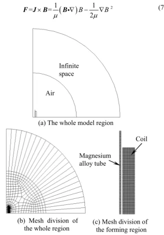
The model region and the mesh division of electromagnetic forming are given in Fig. 3. The PLANE53 elements are applied to magnesium alloy tube, air and induction coil. In order to reduce computational load and to ensure accuracy, INFIN110 element is applied to the outside of air element. The computational region is 1/4 of experimental region with symmetry. The parallel and vertical boundary conditions of magnetic lines of force satisfy Eq. (4) and Eq. (5) on computational region boundary. Electromagnetic force acting on magnesium alloy tube is obtained from Eq. (7).
(
)
21 1
= =
2
B B
μ μ
× i∇ − ∇
F J B B
(7)
Figure 3. Model region and mesh division of electromagnetic forming.
Results and Discussions
The electromagnetic forming process of magnesium alloy tube is essentially the instantaneous discharge forming process of the pulse capacitor. When 2
4
R L C the frequency of current through the induction coil is ω=1 LCand the current reaches the maximum at tmax=π LC 2 (He, 1990). L = 0.0075 mH is a
measured value, and tmax=0.08ms is a calculated value. Transient analysis is applied to numerical simulation. The simulated result is given in Fig. 4. Strong induced magnetic field and electromagnetic force are generated between magnesium alloy tube and induction coil at the moment of electromagnetic forming in Fig. 4.
: 0
B B n
Γ ⋅ =
1 Interface Γ
0 J=
2
Ω J=0
1 Ω
: 0
H H n
Γ × =
(b) Mesh division of the whole region
Air
Infinite space
(a) The whole model region
Coil
Magnesium alloy tube
(c) Mesh division of the forming region
F,
1kN
(b) 4.4kV
B, T
(a) 4.4kV
B, T
Electromagnetic Field Simulation and Crack Analysis of Electromagnetic Forming of Magnesium Alloy Tube
J. of the Braz. Soc. of Mech. Sci. & Eng. Copyright © 2011 by ABCM January-March 2011, Vol. XXXIII, No. 1 / 43
Figure 4. Magnetic flux density and electromagnetic force during electromagnetic forming.
The interaction between the magnesium alloy tube and induction coil is strengthened with the input voltage increase. However, the distribution of induced magnetic field and electromagnetic force are basically unchanged. The stress acting on the wall of magnesium alloy tube exceeds the fracture strength of magnesium alloy at input voltage of 5.2 kV and 4.8 kV by computing. The stress exceeds yield strength of magnesium alloy, and do not reach the fracture strength at input voltage of 4.4 kV.
Figure 5. Magnesium alloy tube of electromagnetic forming.
Figure 6. Stress-strain state of magnesium alloy tube.
The results of electromagnetic forming at input voltage of 5.2 kV, 4.8 kV and 4.4 kV are shown in Fig. 5. Test tube at input voltage of 5.2 kV produced a larger deformation. The crack in the middle of the deformation zone is mainly longitudinal and the crack at two ends of the deformation zone is oblique, shown in Fig. 5(a).The crack of test tube at input voltage of 4.8 kV is oblique at one end of the deformation zone, which is comparatively small, and longitudinal at the other end of the deformation zone, shown in Fig. 5(b). The following results are obtained by the analysis of the above two sets of experiments: 1) Diameter shrinkage of tube is large. It is shown that strong radial pressure and the circumferential stress σθact on the test tube. 2) The crack is mainly longitudinal. It is shown that the distributions of σr and σθare inhomogeneous along circumferential
direction. The test tube showed longitudinal crack with brittleness of magnesium alloy at room temperature. 3) The test tube presents oblique crack at the end of deformation zone. It is shown that the test tube presented a longitudinal crack, and, at the same time, σr of
inhomogeneous axial distribution and σzact on the end of deformation
zone.
The qualified tube is obtained with electromagnetic forming at input voltage of 4.4 kV, shown in Fig. 5(c). The deformation of tube is homogeneous, with no cracks. The maximal diameter shrinkage is 10%. Deformation is inhomogeneous at two ends of the deformation zone. The stress state at the wall of tube is three-dimensional. Its stress-strain state is shown in Fig. 6(a,b). The deformation in the middle of the deformation zone is homogeneous. Its stress state is the plane stress with σθand σr , and its stress-strain state is shown in
Fig. 6(c,d). Under the condition of homogeneous deformation, the relationship between σθ and σr
is given by the equation:
2 rD t θ
σ = σ
(8)
where, D is the outer diameter of tube and t is the wall thickness of tube. According to the corresponding rules of the stress and strain, the sequence of strain increment is consistent with the sequence of stress increment. During electromagnetic forming of tube, axial strain increment
z
dε is expressed:
( )
2
z r
d
dε = − σε σθ+σ
(9)
where, σ
is the equivalent stress,
dεis the equivalent strain
increment. Both σθ and σr in electromagnetic forming of tube are
less than zero, i.e. σθ +σr <0 , dεz > 0 , εz > 0 , and
r
θ
σ σ
.
We have εθ<0, εr>0, namely, tube length increases,tube diameter reduces, and tube wall thickness increases (Lu, 2006).
Figure 7. Coordinate system of strain measurement.
σ
zσ
θσ
r(a) Stress at two ends
ε
zε
rε
θ(b) Strain at two ends
σ
θσ
r(c) Stress in the middle
ε
zε
rε
θ(d) Strain in the middle (a) 5.2kV (b) 4.8kV (c) 4.4kV
0
B, T
(e) 5.2kV
F,
1.3kN
(d) 4.8kV
F,
1.9kN
Z. F. Wang and F. X. Piao et al.
44
/
Vol. XXXIII, No. 1, January-March 2011 ABCMFigure 8. Strain distribution of tube.
Conclusions
1) The electromagnetic field and force field during electromagnetic forming were simulated by ANSYS software. The simulation result is consistent with the electromagnetic forming experiment of the AZ31 magnesium alloy tube. The distributions of electromagnetic field and force field are very similar on the condition of three kinds of input voltages.
2) Stress-strain state of tube forming was analyzed. It is shown that the cause of oblique crack of tube is σr of axial inhomogeneous
distribution and σz, and the cause of longitudinal crack is σr
and
σθof inhomogeneous distribution in circumferential direction.
Acknowledgement
The authors would like to thank the referees for their helpful comments.
References
Le, Q.C., Zhang, J.X., Cui, J.ZH., 2002, “Magnesium Alloys: Current
Status of Their Forming Processes and Applications”, Materials Review,
Vol. 16(12), pp. 12-15.
Chen, ZH.H., Liu, J.W., Chen, D., Yan, H.Ge., 2008, “Deformation mechanisms, current status and development direction of superplastic
magnesium alloys”, The Chinese Journal of Nonferrous Metals, Vol. 18(2),
pp. 193-200.
Svendsen, B., Chanda, T., 2005, “Continuum thermodynamic formulation of models for electromagnetic thermoinelastic solids with
application in electromagnetic metal forming”, Continuum Mechanics and
Thermodynamics, Vol. 17(1), pp. 1-16
Jimbert, P., Ulacia, I., Fernandez, J.I., Eguia, I., Gutierrez, M., Hurtado, I., 2007, “New Forming Limits For Light Alloys By Means Of Electromagnetic Forming And Numerical Simulation Of The Process”,
CP907, 10th ESAFORM Conference on Material Forming, pp. 1295-1300.
Revuelta, A., Larkiola, J., Korhonen, A.S., Kanervo, K., 2007, “High Velocity Forming of Magnesium and Titanium Sheets”, CP907, 10th ESAFORM Conference on Material Forming, pp. 157-162.
Liu, P., 2008, “The Experimental Research on Electromagnetic Forming of Magnesium Alloy Sheet”, WUHAN University of Technology, School of Materials Science and Engineering, Master’s Thesis, 1-54.
Karch, C., Roll, K., 2005, “Transient simulation of electromagnetic forming of aluminium tubes”, Sheet Metal 2005 – Proceedings of the 11th International Conference, SheMet'05, pp. 639-646.
Oszkár, B., Preis, K., 1989, “On the Use of the Magnetic Vector
Potential in the Finite Element Analysis of Three-Dimensional Eddy Currents”, IEEE Transactions on Magnetics, Vol. 25(7), pp. 3145-3159.
Biro, O., 1988, “Use of A Two-Component Vector Potential for 3-D
Eddy Current Calculations”, IEEE Transactions on Magnetics, Vol. 24(1),
pp. 102-105.
He, X.CH., Hu, Q.P., Zhang, Y.J., 1990, “Discussion on Some Problems of Pulsed Magnetic Fields for Metal Forming”, China Metal Forming Equipment & Manufacturing Technology, Vol. 6, pp. 8-12.
Lu, Y.J., 2006, “Research on Uniformity of Tube Electromagnetic Forming”, HARBIN Institute of Technology, School of Materials Science and Engineering, Master’s Thesis, pp. 47-52.
-50 -40 -30 -20 -10 0 10 20 30 40 50
0.00 0.01 0.02 0.03 0.04 0.05 0.06 0.07 0.08
距中心距离 /mm
应变
e
St
ra
in
Distance from the center /mm (b) Axial strain (a) Circumferential strain
-50 -40 -30 -20 -10 0 10 20 30 40 50
-0.10 -0.09 -0.08 -0.07 -0.06 -0.05 -0.04 -0.03 -0.02 -0.01 0.00
应变
e
距中心距离 /mm
St
ra
in