Maria de Lourdes C. Barros
[email protected] University Federal of Pará Mechanical Engineering Post-Graduation Program PPGEM/ITEC/UFPA 66075-110 Belém, Pará, BrazilManoel José dos Santos Sena
[email protected]Amazon High Studies Institute 66055-260 Belém, Pará, Brazil
André Luiz Amarante Mesquita
[email protected] University Federal of Pará School of Mechanical Engineering FEM/ITEC/UFPA 66075-110 Belém, Pará, BrazilClaudio José C. Blanco
[email protected] University Federal of Pará School of Sanitary and Environmental Engineering FAESA/ITEC/UFPA 66075-110 Belém, Pará, BrazilYves Secretan
[email protected] INRS-ETE – Institut National de la RechercheScientifique G1K 9A9 Québec (Qc), CANADA
A
Water Flow Pattern Analysis of
Guajará Bay – Amazon Estuary –
Brazil
This work describes the steps required to construct a hydrodynamic model of the Guajará Bay, using Geographic Information Systems and the Finite Element Method. An overview of the problem that motivates this modelling procedure, i.e., the pollutant dispersion, is presented. The computer software used is then discussed, stressing the links between the data model entities. The calibration procedure is described. The methods used to obtain field data and the results obtained are presented, alongside the main flow patterns of the water. The simulations and applications of the model are discussed at the end of the paper. Keywords: Guajará Bay, hydrodynamic model, Geographic Information Systems, Finite Element Method, pollutant dispersion
Introduction
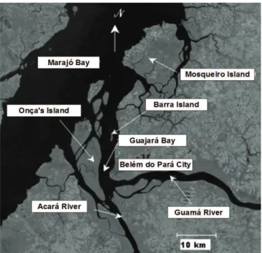
1The Guajará Bay delimits the city of Belém, capital of the Pará State, in the Amazon Region, as shown in Fig. 1. It is located, approximately, between the parallels 1°22’S and 1°30’S and the meridians 48°25’W and 48°35’W. Its distance to the Atlantic Ocean is about 120 km. The formation takes place in the confluence between the rivers Guamá and Acará. It extends towards the North up to the island of Mosqueiro. Finally, it merges to the Marajó Bay, which is connected to the Atlantic Ocean.
Belém was founded in 1616, and it is the city from which the occupation of the Amazon Region has begun. From its privileged location, it is a very important point of distribution of products to and from all the Amazon Region and has a growing industrial capacity.
There is very little knowledge about the flow patterns in this system, despite the fact that the city of Belém has the biggest population density in all the Amazon Region. The total population of the city is about 1,500,000 peoples. This leads to difficulties in the city water and sewer management. It must be outlined that there is no sewer treatment station in the city. All the used waters are rejected to Guajará Bay or to the Guamá River.
A growing level of pollution has been observed in the beaches situated by the islands near the city of Belém. This fact has been influencing negatively the tourism in the region. The origin of this pollution is supposed to be the city of Belém. But to discover the origin of the problem, it is necessary to dispose of a tool able to analyze the trajectory followed by the pollutant masses in the Guajará Bay.
Paper accepted July, 2010. Technical Editor: Demétrio Bastos Neto
Figure 1. Satellite image showing the location of the Guajará Bay.
This text describes the methodology that used to implement the hydrodynamic modeling of the Guajará Bay, including its calibration.
Nomenclature
D = deformation tensor component, N/m2
F = volume force, N
g = acceleration of gravity, m/s2
H = depth of the water column, m
h = water level, m
L = mixing length, m
n = Manning coefficient, dimensionless
q = flow rate, m3/s
qG = modulus of the specific flow rate,
t = time, s
x = direction x of the Cartesian Coordinate System
y = direction y of the Cartesian Coordinate System
Greek Symbols
∂ = relative to partial derived
ρ = water density, kg/m3
τ = Reynolds stress tensor, N/m2
υ = viscosity
Subscripts
cx relative to coriolis force in x cy relative to coriolis force in y
i relative to plan of τ and to plan of D, and relative to direction of partial derived
j relative to plan of τ and to plan of D, and relative to direction of partial derived
m relative to mixing t relative to turbulent x relative to direction x y relative to direction y wx relative to wind force in x wy relative to wind force in y
Hydrodynamic Modeling in Environmental Studies
The characterization of the sensibility of areas subject to environmental damages can be carried out through the integration of hydrodynamic information with geographical information systems. The work of Castro et al. (2003) shows the application of this type of technique in the coast of Rio Grande do Norte – Brazil. The determination of the flow patterns, specially the current direction, is one of the most important aspects taken into account in the determination of environmental sensibility, besides the geomorphology and the vegetation of the site. So, the better is the definition of the flow, the better is the environmental sensibility definition.
The knowledge of the hydrodynamic behavior of the water bodies is a basic aspect to the environmental management to be correctly fulfilled. This can be exemplified by the work of Wang et al. (2003). In this case, a hydrodynamic model coupled to a salinity model of the Biscayne Bay, in Florida, United States, is used to analyze the time and spatial distributions of larvae of aquatic species. The distribution of the larvae is proportional to the salinity, which is directly linked to the water flow.
Hydrodynamic Model
The first step of a water quality modeling is to know the time variation of the flow in each point of the water body. To accomplish
this task, a hydrodynamic model is necessary. In this study, the adopted model is two-dimensional depth integrated type. In this case, the mass conservation and momentum equations are discretized in the longitudinal – transversal plane and integrated in the depth, or vertical direction. The problem then becomes two-dimensional and the values obtained for velocities and elevations of water are means in the vertical direction. These models are also called Saint Venant models. The conditions to be filled so that they provide good results are (Heniche et al., 2000):
- The water column is mixed in the vertical direction and the depth is small compared to the width and the length of the water volume;
- The waves are of small amplitude and long period (tide waves). The acceleration’s vertical component is negligible, allowing the hydrostatic pressure approximation.
The adaptation of these models to the study of the hydrodynamic behavior of the Guajará Bay must be analyzed by stressing its main characteristics (Pinheiro, 1987): absence of thermal stratification; small salinity variations; small velocity components in the vertical direction; circulation dominated tidal currents (with tidal amplitudes between 3.0 m and 2.5 m). These characteristics allow us to say that a Saint-Venant model is able to supply satisfactory results for the flow patterns in the Guajará Bay.
The equations (1) to (3) are the conservative form of the Saint-Venant equations. The first one is the mass conservations equation while the two others are the momentum for the fluid:
0 = ∂ ∂ + ∂ ∂ + ∂ ∂ y q x q t
h x y (1)
∑
= ∂ ∂ + ∂ ∂ + ∂ ∂ x y x x x x F y H q q x H q q tq (2)
∑
= ∂ ∂ + ∂ ∂ + ∂ ∂ y y y x y y F y H q q x H q q tq (3)
x and y are the directions of the Cartesian Coordinate System used,
qx and qy are the flow rate in the x and y directions, respectively, t is
the time, h is the water level, H is the depth of the water column and
Fx and Fy are the volume forces in the x and y directions,
respectively.
Fx and Fy are calculated by equations (4) and (5):
(
)
(
)
wx cx xy xx x x F F y H x H H q q g n x h gH F + + ⎟⎟ ⎠ ⎞ ⎜⎜ ⎝ ⎛ ∂ ∂ + ⎟ ⎠ ⎞ ⎜ ⎝ ⎛ ∂ ∂ + − ∂ ∂ − =∑
ρ1 τ ρ1 τ3 / 1 2 G (4)
(
)
(
)
wy cy yy yx y y F F y H x H H q q g n y h gH F + + ⎟⎟ ⎠ ⎞ ⎜⎜ ⎝ ⎛ ∂ ∂ + ⎟⎟ ⎠ ⎞ ⎜⎜ ⎝ ⎛ ∂ ∂ + − ∂ ∂ − =∑
ρ1 τ ρ1 τ3 / 1 2 G (5) where g is the acceleration of gravity, n is the Manning coefficient,
qG is the modulus of the specific flow rate, ρ is the density of the water, τijis the Reynolds stress tensor, Fcx and Fcy are the Coriolis
forces in x and y directions, respectively, and Fwx and Fwy are the
wind forces in the x e y directions, respectively.
obtained from the geomorphological aspects of the bottom of the Guajará Bay (Pinheiro, 1987).
P01
P05
P03
P04 P12
P14 P06
The following boundary conditions were adopted:
- In the solid frontiers – there was no flow in or out by the solid boundaries;
- In the liquid frontiers – there was imposed tide elevation, obtained through field measurements.
The turbulence model used was the mixing length. This approach considers the distance from the wall, where the size of the turbulent structures is not influenced by the wall itself. This model assumes a balance between the energy creation and dissipation. In this case, the turbulent viscosity is given by:
ij ij m
t L 2DD
2
=
υ
(6)
υt is the turbulent viscosity; Lm is the mixing length; Dij are the ij
components of the deformation tensor, given by:
⎟ ⎟ ⎠ ⎞ ⎜
⎜ ⎝ ⎛
∂ ∂ + ∂ ∂ =
i j
j i ij
x U x U D
2
1 (7)
Figure 2. Scale positions in Guajará Bay.
i
U is the mean velocity in the i direction.
A detailed treatment of the different methods used in this study can be obtained in the works of Padilla et al. (1997); Morin et al. (2000); Secretan and Leclerc (1998) and Heniche et al. (2000).
Applications to the Guajará Bay
As a initial step in the modeling process, an assembly of bathymetry data from nautical maps of the Marinha do Brasil and field measurements carried out by the Administração das Hidrovias da Amazônia Oriental, AHIMOR, were used to build up a terrain numerical model.
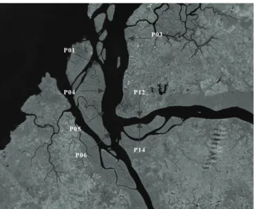
To measure the tide levels, six stations were used. Figure 2 plots their positions. There were used fixed immersed scales.
Figure 3 shows one of these stations. The measures were taken in September 2004. The hypothesis, stating that the water mean level was the same within the domain, was assumed for the vertical positioning of the scales. As the water level differences between the limits of the model, due to the tides, are up to 60 cm, the flow inertial effects are much greater than the differences in the water mean level.
The mean level used was those considered by the Marinha do Brasil for the Belém’s Port, 1.81 m. All the measured levels were reduced to it. The measures were obtained in periods of 13 hours, each 30 minutes. Figure 4 shows the water levels measured.
Figure 3. Mounted scale on point 05.
2.0m 1.0m 2.5m 0.8m 2.9m 1.81m 1.81m 1.81m 1.81m 1.81m
The analysis of Fig. 5 allows some observations about the tide wave displacement in Guajará Bay. For example, the delay between the levels measured in points 3 and 12 is about 50 minutes. In the high and low tide, the water level is approximately the same in the entire domain. Meanwhile, the level difference between points 3 and 12 reaches 60 cm when tide growth rate is highest. As the distance between the points is about 20 km, indicating a declivity of 3 cm per km. This illustrates how strong the dynamic tide effects are in the flow in this estuary.
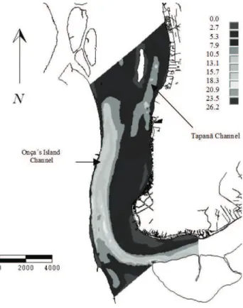
Figure 6. Depths in Guajará Bay (meters).
The tidal curve is more inclined in the flood than in the ebb. This is due to the tidal wave speed, which depends on the water depth. The tidal wave crest is traveling faster than the tidal wave through. It is also possible to verify the little damping in the region. The waves measured in the different stations have quite the same amplitude.
To calibrate the model, the points 1, 3, 6 and 14 were used to fix the boundary conditions. The points 4 and 5 were used as calibration control points.
Figure 6 shows the depths in the Guajará Bay. It can be observed that there are two main channels. The Ilha das Onças Channel follows the contour of the island of same name. The Tapanã Channel is at the east side of Da Barra Island (Fig. 1). The area surrounding Belém is, on the other hand, very sandy.
The methodology to obtain the numerical solution was split into two steps. A stationary simulation was conducted, in order to obtain an initialization condition for the instationary calculation. For the stationary simulation, the water levels, at the north frontier, and flow rates, at the Guamá and Acará rivers, were imposed as boundary conditions. At this point, the mesh density was adjusted. The chosen mesh is showed in Fig. 7. It is composed of 13,809 nodes and 6,685 triangular elements. The isotropic frontal algorithm was used to generate this mesh. The distance parameter was set to 140 m.
Figure 7. Finite element mesh.
To perform the instationary simulation, the converged solution for the stationary one was considered as initial solution. From this moment, the boundary conditions specified were the measured water levels. They were repeated over each tidal cycle. A time step of five minutes was used. Two tidal cycles were let to develop before the results began to be stored. This was necessary to damp the fluctuations due to the new imposed boundary conditions. The Manning coefficient was the calibration parameter of the model. The initial values for them were obtained by the analysis of the work of Pinheiro (1987).
Results and Discussions
Figures 8 and 9 show the comparison between the calculated and measured water levels. A good correlation can be observed, considering the amplitudes, period and phase change of the tide wave.
Figure 5. Measured water levels. 0
0.5 1 1.5 2 2.5 3 3.5
7:
00
8:
00
9:
00
10:
00
11:
00
12:
00
13:
00
14:
00
15:
00
16:
00
17:
00
18:
00
19:
00
hours
w
a
ter l
evel
[m]
0 0.5 1 1.5 2 2.5 3 3.5
14:24 16:48 19:12 21:36 0:00 2:24 t(h) h( m) 0 0.5 1 1.5 2 2.5 3 3.5
14:24 16:48 19:12 21:36 0:00 2:24 t(h)
h(
m)
Figure 8. Comparison between the measured (•) data and simulated (o) results in point 4.
Figure 9. Comparison between the measured (•) data and simulated (o) results in point 5.
-2 -1.5 -1 -0.5 0 0.5 1 1.5 2 14 :42 15 :32 16 :22 17 :12 18 :02 18 :52 19 :42 20 :32 21 :22 22 :12 23 :02 23 :52 0: 4 2 1: 3 2 2: 2 2 Time (hours) E b b V e lo c ity ( m/s ) F lo o
d Point 1
Point 3 Point 5 Low Tide High Tide -2 -1.5 -1 -0.5 0 0.5 1 1.5 2 14: 42 15: 32 16: 22 17: 12 18: 02 18: 52 19: 42 20: 32 21: 22 22: 12 23: 02 23: 52 0: 42 1: 32 2: 22 Time (hours) E b b V e lo c it y ( m /s ) F lo o
d Point 1
Point 3 Point 5 Low Tide High Tide -2 -1.5 -1 -0.5 0 0.5 1 1.5 2 14 :4 2 15 :3 2 16 :2 2 17 :1 2 18 :0 2 18 :5 2 19 :4 2 20 :3 2 21 :2 2 22 :1 2 23 :0 2 23 :5 2 0: 42 1: 32 2: 22 Time (hours) E b b V e lo c it y ( m /s ) F lo o
d Point 7
Point 8 Low Tide High Tide -2 -1.5 -1 -0.5 0 0.5 1 1.5 2 14: 42 15: 32 16: 22 17: 12 18: 02 18: 52 19: 42 20: 32 21: 22 22: 12 23: 02 23: 52 0: 42 1: 32 2: 22 Time (hours) E b b V e lo c ity ( m /s ) F lo o d Point 7 Point 8 Low Tide High Tide
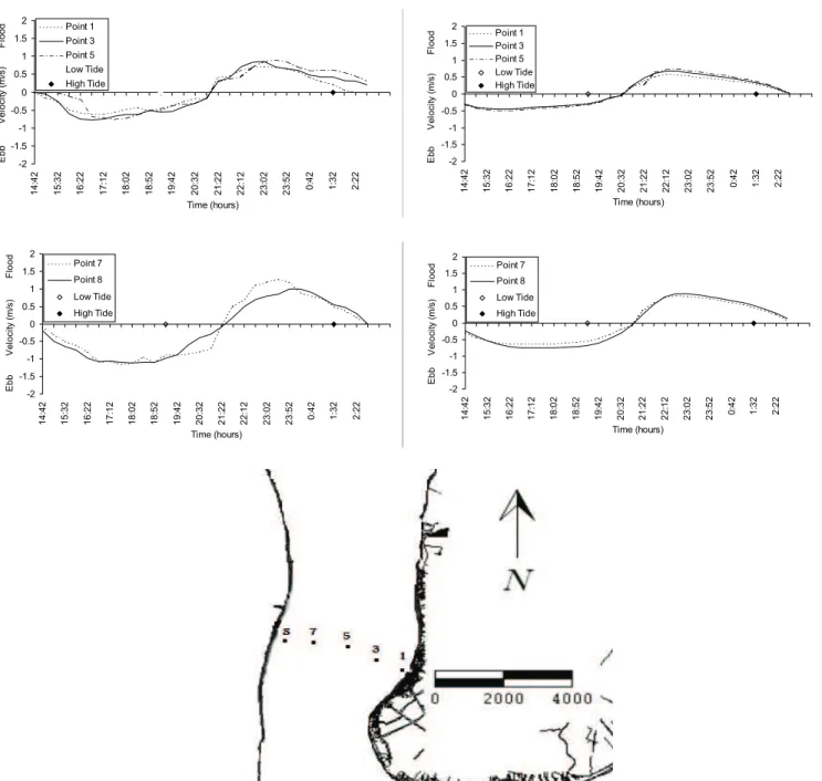
Figure 10. Comparison between the velocities measured at one meter d at t e right. In the bottom center, the location of the measuring points.
To perform a comparison of the velocity field, a measurement procedure described by Pinheiro (1987) and conducted by the Belém’s Port was considered. The water levels and velocity measures were taken in the same month of the year, but the latter took place in 1983. These were the only data available and were considered here for a qualitative comparison. Figure 10 shows the spatial location of the probes and the measured and simulated values of the velocity modulus. The probes were located far from the boundary conditions, so that the flow is completely developed when it reaches this region. It can be also observed that there are strong velocity gradients in this location.
In the analysis of Fig. 10, it must be considered that the measured velocities were taken at one meter depth and the simulated ones are integrated in the vertical direction. Indeed, the measured velocities shall be greater in modulus than the simulated. We can observe this behavior in Fig. 10. Also, the relative positions of highest and lowest water levels in the considered section present a good agreement between the two sets of data. This indicates that the model represents adequately the global mass transfers in the domain.
It is possible to notice that the velocity behavior is more symmetric in the region of points 1, 3 and 5, near the Belém Harbor. In points 7 and 8, the velocities during the ebb last longer at high modulus than in the flow. It indicates that the liquid flow rate in the region of points 7 and 8 lets the water of Guamá and Acará Rivers flow towards the Marajó Bay. On the other hand, the region near points 1, 3 and 5 tends to have a small liquid flow rate. This shows that the site of Belém Harbor is not adequate to receive sediments from the drainage channels or pollutants, because they will tend to rest confined in this domain for a longer time than if they were released in the region near points 7 and 8.
The higher velocity modulus in points 7 and 8 can be explained by the fact that the Ilha das Onças Channel provides continuity for the Guamá River Main Channel. The bathymetry of these channels forms a preferable way for the flow.
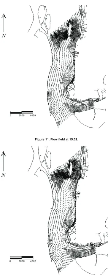
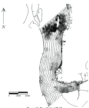
The sequence of figures from 11 to 14 shows the vector field representing the velocity directions at a few points of the finite element mesh used to perform the simulations.
At 15:32, in Fig. 11, the flow shows an ebb tide configuration, with the velocity vectors directly towards the north. In this case, a relatively low velocity zone is noted by the Belém Harbor.
At 20:32, according to Fig. 12, the tide begins to change from ebb to flow. At this moment, the velocities are very low in almost all the domain. It is interesting to note that the tide is not at its lowest level. This can be explained by the inertial effects of the flow, which causes a time lag between the lowest level of the tide and the flow reversion. This reversion begins in the Belém side of the Guajará Bay, creating two vortices’ regions near the Belém Harbor and just in the confluence between the Guamá River and the Guajará Bay. These flow features are known from the locals of Belém and are present in the drawn arrows of Fig. 10. Their presence in the simulated results shows that the model reproduces the main characteristics of the flow when this state is reached.
Twenty-five minutes later, as shown in Fig. 13, the vortices are translated to the east, towards the Ilha das Onças channel. Finally, at Fig. 14, the flow is fully developed.
Figure 11. Flow field at 15:32.
Conclusions
The hydrodynamic model of the Guajará Bay developed in this work showed a good agreement when compared with measured water levels and flow velocities.
Using the results obtained from the model, different studies such as sediment transport, water quality and pollutant transport can be conducted. The model can also be extended to cover a greater area to consider more global phenomena.
Despite the fact that the main sewer drainage channels pour their waters at the Belém's shoreline, the low intensity vector field in these places is not convenient to pollutant dispersion. The effects of the turbulent diffusion are weakened, as they are proportional to the velocity field complexity and intensity. One of the applications of this hydrodynamic model as a basis for pollutant dispersion studies is to evaluate the best moments to open the channels to let the flow pass.
Acknowledgements
The authors wish to thank CNPq – “Conselho Nacional de Desenvolvimento Científico e Tecnológico”, of the Brazilian Ministery for Science and Technology, through the dossier n. 550461/01-9 (PNOPG/2002); and SECTAM – “Secretaria de Ciência e Tecnologia”, of the State of Pará, through the dossier 078/01-SECTAM/FUNTEC/IESAM for the financial support provided.
Figure 13. Flow field at 20:57.
Figure 14. Flow field at 22:12.
References
Castro, A.F., Amaro. V.E. and Vital, H., 2003, “Desenvolvimento de um banco de dados geográficos em um ambiente SIG e sua aplicação na elaboração de mapas de sensibilidade ambiental ao derramamento de óleo em áreas costeiras do Estado do Rio Grande do Norte”, Proceedings of the XI SBSR, Belo Horizonte, Brazil, pp. 1533-1540.
Heniche, M.A., Secretan Y., Boudreau P. and Leclerc, M., 2000, “A two-dimensional finite element drying-wetting shallow water model for rivers and estuaries”, Advances in Water Resources, Vol. 23, pp. 359-372.
Morin, J., Leclerc, M., Secretan, Y. and Boudreau, P., 2000, “Integrated two-dimensional macrophytes-hydrodynamic modeling”, Journal of Hydraulic Research, Vol. 38, No. 3, pp. 163-172.
Padilla F., Secretan, Y. and Leclerc, M., 1997, “On open boundaries in the finite element approximation of two-dimensional advection-diffusion flows”,
International Journal for Numerical Methods in Engineering, Vol. 40, No. 13, pp. 2493-2516.
Pinheiro, R.V.L., 1987, “Estudo Hidrodinâmico e Sedimentológico do Estuário Guajará”, Master Thesis, Universidade Federal do Pará, Belém, Brazil.
Secretan, Y. and Leclerc, M., 1998, “Modeleur: a 2D hydrodynamic GIS and simulation software”, Proceedings of the Hydroinformatics-98, Copenhagen, Denmark, pp.1-18.