Liquidity, Business Cycles and Monetary Policy: a Simulation

Liquidity, Business Cycles and Monetary

Policy: a Simulation

Pedro Castro Henriques

January 2010

Abstract

In Kiyotaki and Moore (2008) the authors develop a model in which di¤erences in the liquidity of distinct assets create a link between asset prices and macroeconomic aggregates. Their goal is to build a work-horse model that incorporates liquidity as the cause for the circulation of money, in a dynamic stochastic general equilibrium (DSGE) environ-ment, close enough to the real business cycle (RBC) framework, and thus, suitable for studying monetary policy. In this article, I am interested in studying how this framework can be used to understand the e¤ects of liquidity and technology shocks in the U.S. economy. I calibrate their model and study the impact of adding up liquidity constraints on its RBC performance. I …nd that liquidity constraints have a remarkable impact on the volatility of investment and consumption. Moreover, I conclude that, in this context, asset prices’ volatility is explained as a natural feature of a monetary economy when hit by liquidity shocks.

Acknowledgements: I thank Professor Nobuhiro Kiyotaki for his insightful comments on the results obtained; my orienteer and co-orienteer, respectively Professor Pedro Teles and Professor Francesco Franco, for their support throughout the elaboration of this article; and Professor Wouter Den Hann for teaching me how to use Dynare and Matlab, the simulation package adopted in this article.

1 Introduction:

In Kiyotaki and Moore (2008) - henceforth, KM - the authors develop a model

in which di¤erences in the liquidity of distinct assets create a link between

asset prices and macroeconomic aggregates. Their ultimate goal is to build

a workhorse model that incorporates liquidity as the central cause for the

existence of money, in a Dynamic Stochastic General Equilibrium (DSGE)

environment, close enough to the Real Business Cycle (RBC) framework, and

thus, suitable for studying monetary policy.

KM di¤ers from the usual monetary models in the sense that money is

neither de…ned in a reduced-form way, as conventionally done in

Cash-in-Advance and Money-in-Utility models, nor assumed to result from a search

environment, as in the prevailing matching models1. The problem with the

…rst type of models, is that they impose the usage of money rather than explain

the causes that justify its circulation. This is not the case with matching

models, in which money arises endogenously. However, this type of models is

usually not suitable for doing monetary policy, given that tractability is often

lost when too rigid assumptions are relaxed2.

In KM instead, money circulation is not imposed (meaning that money,

as an asset, plays no particularly di¤erent role in the economy) and markets

are competitive. However, in this model the economy is subject to liquidity

constraints, which ultimately de…ne whether money is used or not.

In the model of KM there are two types of agents - workers and

entre-preneurs. Two types of assets are transacted: money (in …xed supply) and

capital or equity claims of capital (which supply depends on investment and

depreciation). While workers play a passive role in this economy, either

con-1_{See Lucas and Stokey (1987) and Christiano et al.(1997) for examples of Cash-in-Advance}

models. Kiyotaki and Wright (1989) and Kocherlakota (1998) illustrate the nature of match-ing models.

2_{Lagos and Wright (2005), Aruoba, Waller and Wright (2009) and Huang and Wright}

suming or saving their income (in the form of money or equity), entrepreneurs

have access to a production technology and are subject to an iid investment

opportunity shock. The fraction of entrepreneurs hit by the shock, have the

opportunity to invest in a technology that transforms one unit of output in

t into one unit of capital in t+ 1. Given that, only a percentage of entre-preneurs face these investment opportunities, there is a need for transferring

resources from those who do not have been hit by the shock (savers), to those

who have (investors). In practice, investors sell equity claims on the output

return, resulting from the newly produced capital, at market price qt, in

or-der to …nance their investment. Crucially, investors are needed to employ

the newly produced capital and provide the return on equity to its creditors.

However, they are not necessarily able to commit to do so. Hence, this limited

commitment constraint implies that investors can only pledge a given fraction

2(0;1)of the newly issued capital. This constitutes a borrowing constraint, in the sense that investors cannot completely leverage the investment

oppor-tunity. In other words, funds are not fully transferred from savers to investors

and these face the need to …nance the investment with their own funds. At

this point, liquidity plays its decisive role: in fact, while money holdings are

fully convertible into output goods at market price pt, equity (either in the

form of own capital stock or equity claims on others’ capital stock) is only

convertible into output goods up to a fraction '_t2(0;1), at market price q_t, each period.

Whether money plays a role in this economy is de…ned by how stringent

and '_t are. The reason for this lies on the fact that entrepreneurs face a trade-o¤ between holding money and equity: money pays a low return but

is completely liquid, whereas equity pays a high return but is only partially

signi…cant ( and'_tare close enough to one), then the economy is su¢ciently liquid and there is no need to hold the lowest return asset (money). Hence,

in this context money serves the sole purpose of lubricating the economy. If

such purpose is not needed (the economy is already su¢ciently lubricated)

then money circulation is ruled out. Instead, if liquidity is scarce, money

arises endogenously to lubricate the economy and facilitate the ‡ow of funds

between savers and investors.

Notice that, even though the authors successfully endogenize money, they

do so by creating a reduced-form structure for the liquidity constraints present

in the model. In fact, the resaleability constraint '_t - similarly to the cash-in-advance constraint or the money-in-utility formulation - lacks structural

robustness. More concretely, note that '_t is de…ned as a Markov stochas-tic process, so that shocks to the resaleability of equity are present in the

model. This is an approach to track the sudden liquidity shortage that has

characterized the recent …nancial turmoil, but we can see right away that it

is a poor one. In reality, the formulation of '_t, as de…ned in KM, stipulates that the …rst fraction of old equity holdings is sold at no cost, whereas from

the ('_t)th fraction onwards, the investor bears an in…nite transaction cost of selling equity. Clearly this is an unreasonable cost structure, which lacks

mi-croeconomic fundament3. It is, however, beyond the scope of KM to justify

the microeconomic foundations of'_t, instead it focuses on understanding the e¤ects of liquidity shocks.

Notwithstanding the above, this innovative speci…cation of money and

liq-uidity in a DSGE framework, not only successfully justi…es seemingly

para-doxical macroeconomic facts, as natural features of a monetary economy that

is subject to liquidity shocks, but also allows for the performance of monetary

3_{This precise fact is referred by John Moore in Claredon Lectures 2 - Liquidity, business}

policy in a tractable environment4_.

The RBC literature is nowadays particularly interested in exploring the

capacity of state-of-art models, to produce real business cycle statistics that

are in line with the ones observed in the data. The better their performance,

the more con…dent one can be when using these models for monetary policy

analysis. New-keynesian models like the ones presented in Christiano, Martin

Eichenbaum, and Charles L. Evans (2005) or in Frank Smets and Raf Wouters

(2007), are equipped to produce time series that can remarkably mimic the

data. In fact, these models are so e¤ective in …tting the data that, as I

write this article, the European Central Bank is using a version of Smets and

Wouters (2007) to inform its monetary policies. Nonetheless, it is not

consen-sual among macroeconomists whether we should support or disencourage the

usage of New-keynesian models for monetary policy purposes. In fact, a great

number of economists …ercely believe that New-keynesian models are not yet

useful for policy analysis, as defended by V.V. Chari, Patrick J. Kehoe and

Ellen R. McGrattan (2008). The main critique being faced by New-keynesian

economists is that they include too many dubiously structural parameters and

reduced-form shocks, that are manifestly inconsistent with microeconomic

ev-idence. Neoclassical economists, instead, refuse to include such short-cuts in

their models, for the sole purpose of improving their RBC performance, on

the grounds that these constitute a severe incongruence with the data, which

cannot be ignored when doing policy analysis. From a Neoclassical

perspec-tive, as long as this incongruence prevails, New-keynesian models should not

be considered reliable for policy analysis, and thus should not be used by

central authorities to quantitatively inform their policy-making. Until then,

qualitative rules-of-thumb should instead be used.

The model proposed by KM is, in its essence, a congregation of

di¤er-4_{These paradoxes include the low risk-free rate, the low rate of participation in asset}

ent streams of thought and economic theories. Its structural core is a basic

Neoclassical model, perfectly competitive and absent of nominal frictions. In

this sense this model, avoids the usual criticisms faced by New-keynesian

pro-ponents, in what concerns the pro‡igacy of dubiously structural shocks and

reduced-form structures that are poorly microfounded5. In fact, the model

of KM includes only one typically New-keynesian reduced-form shock - the

liquidity shock '_t - as a short-cut for modelling the resaleability constraint presented in Kiyotaki and Moore (2005). As for the investment decision, it

embodies the Tobin’s q theory, to the extent that investors have an incentive

to invest as long as the market price of equity is higher than its cost(qt>1).

Finally, this model proposes an innovative way of including money in a DSGE

framework, one that focus on the role of money in lubricating the economy,

as the sole cause for its circulation.

Considering the above, despite the reduced-form structure for '_t, the model of KM is essentially a Neoclassical model, with an original modelling of

money and liquidity. My goal is to study to what extent it can contribute to

the RBC literature. More concretely, my ambition is to discernibly understand

how does each feature of the model in KM contribute to changing the RBC

performance of a standard Neoclassical model. In order to do so, I simulate

a sequence of models that are simpler versions of KM, calibrated for the U.S.

economy. In practice, I start by simulating the simplest version of the model

in KM: a standard Neoclassical model, very close to the one presented in King

and Rebelo (1999) - also referred to as KR in what follows. Then, I proceed

step-by-step, adding up new features to this basic framework, at each step

an-alyzing the RBC performance of the model, until I end up with the economy

of KM. My goal is to scrutinize the impact of each new ingredient added, on

the RBC behavior of the model. As we shall see, liquidity constraints have a

5_{Check Chari, Kehoe and McGrattan (2008) for a critical view of how suitable}

remarkable impact on the ability of this model to …t the RBC statistics

ob-served for the U.S. economy. In particular, I show that liquidity constraints

have a very strong impact on the volatility of investment and consumption,

not so much directly, through their impact on the entrepreneurs’ behavior,

but rather indirectly, for the simple fact that they disencourage workers from

participating in the asset market. Moreover, the model of KM justi…es the

paradox of asset prices’ volatility as natural feature of a monetary economy

that is hit by liquidity shocks '_t.

The structure of the rest of this article is the following: in Section 2 I

present, in a summarized way, the model of KM; Section 3 exposes the above

referred Neoclassical de-construction of KM, together with the simulation

re-sults of each simpli…ed model; in Section 4 I explain in detail the calibration

procedure for the original KM model; Sections 5 and 6 include a detailed study

of the shock dynamics in KM and the simulation results for the original KM

model; …nally in Section 7 I present some concluding remarks.

2 The Model:

In the model of KM there are two types of agents - workers and entrepreneurs

- with distinct preferences, although they share the same rate of time

prefer-ence. Entrepreneurs are subject to investment opportunities that allow them

to produce new capital out of consumption goods. Investment opportunities

are independent and identically distributed across entrepreneurs and have a

constant arrival rate 2(0;1). Therefore, at each point in time there exists a fraction of entrepreneurs who have an investment opportunity (investors)

and a fraction 1 who do not (savers). Workers, instead play a passive

role in this economy. They cannot invest as they are assumed not to face

investment opportunities. Hence, they work and either save or consume their

There are three types of assets traded, namely a non-durable consumption

good (output) Y, equity N and moneyM. Money is di¤erent from equity in the sense that it is completely liquid, meaning that it can be transformed into

consumption goods at price p_t with no restrictions (notice that p_t is hereby de…ned as the inverse of the usual price level). On the contrary, equity is the

illiquid asset in this environment, in the sense that it can only be partially

transformed into consumption goods at price qt. The aggregate amount of

money in this economy is set …xed at some quantity M. I proceed by describing this model for each type of agent.

2.1 Workers:

There is a unit measure of workers each with present value utility, at date t, given by:

E0

1

X

t=0

t_{U c}w t

!

1 + (l w

t)1+ (1)

wherecw_t is the consumption level of a typical worker in period tandlw_t is his labour supply in hours. Assume that U[:]is increasing and strictly concave. Workers do not have investment opportunities, which means that their income

relies on the return from their savings and on the wage they get for each hour

worked. Money pays no return, whereas equity provides gross pro…t rate r_t

and depreciates at rate 1 with 2 (0;1). Hence the ‡ow of funds of a worker can be described as:

cw_t +qt ntw+1 nwt +pt mtw+1 mwt =wtlwt +rtnwt (2)

wheremw_t andnw_t are holdings of money and equity respectively andwtis the

real wage rate.

l_tw= wt

!

1

(3)

This is obtained by equating the marginal rate of substitution between

con-sumption and leisure to the real wage.

Given that there exists a unit measure of workers, the resulting aggregate

labour supply is given by:

Lw_t = wt

!

1

(4)

Later it will be proved that, in a neighborhood of the steady state, workers

decide not to save in any kind of asset and thus set their consumption equal

to their entire labour income. From this point onwards I assume this is the

case:

Claim 1: In a neighborhood of the steady state, workers decide not to save

any of their income, thus consuming all earnings resulting from the hours

worked.

cw_t =wtlwt 2.2 Entrepreneurs:

As with workers, there is a unit measure of entrepreneurs with preferences

given by:

E₀

1

X

t=0

t_{log (c}

t) (5)

Each entrepreneur has access to a constant returns to scale (CRS)

tech-nology that produces consumption goods out of capital and labour inputs,

according to a Cobb-Douglas:

yt=At(kt) (lt)1 ; (6)

The capital share of output is denoted by 2(0;1). The output produced by entrepreneurs can both be consumed or saved in either equity or money.

Entrepreneurs employ workers in a perfectly competitive labour market,

which means that one can de…ne the gross pro…t rate r_t as the marginal pro-ductivity of capital:

yt wtlt=rtkt (7)

Given kt, entrepreneurs maximize their gross pro…t net of labour costs

At(kt) (lt)1 wtltwith respect tolt. This gives rise to the aggregate labour

demand:

L_t=K_t (1 )At wt

1

(8)

whereKtis the aggregate capital stock. The labour market clearing condition

is the one that equates Lt to Lwt, from (4) and (8). This implies that the

equilibrium real wage rate is:

w_t= K_t[(1 )A_t]1 !1 + (9)

Once we substitute the equilibrium wage rate above into the expression of

the gross pro…t net of labor costsAt(Kt) (Lt)1 wtLt, we can de…ne this

to be equal to rtKt wherertis:

rt=at(Kt) 1 (10)

where:

at= 1

!

1 +

(At) 1+

+ _;

= 1 +

+ ; (11)

it decreases withKt. Note however that aggregate output, net of labour costs,

Yt =rtKt = at(Kt) is an increasing function of the capital stock. I is also

worth emphasizing that, although on the individual level entrepreneurs have

access to a constant returns to scale technology, on aggregate, this economy has

a decreasing returns to scale production technology. As for the productivity

shockAt it has a positive impact on rtthrough at.

As previously referred, investment opportunities appear to entrepreneurs

with an arrival rate 2 (0;1). These allow them to transform one unit of output in period t into one unit of capital in period t+ 1. Entrepreneurs …nance investment by issuing equity claims on the output produced using the

new capital. They sell these claims forqt units of output and pay one unit of

output for each claim. Hence, entrepreneurs decide to invest as long asqt>1.

Conversely, if q_t<1they prefer not to invest, whereas if q_t= 1 entrepreneurs are indi¤erent between investing and consuming. In this sense, this model

embodies the Tobin’sq theory of investment.

The equity claims pay rt+1 units of output att+ 1, rt+2 att+ 2, 2rt+3

at t+ 3 and so on, for each unit of investment. Investors are not necessarily able to commit to provide these returns on equity to creditors. Due to this

limited commitment constraint, investors are only able to pledge a certain

proportion of their investment. This is called the Borrowing Constraint and

formally states that, investors can only pledge a fraction 2 (0;1) of the newly issued equity i_t. Since the price of the newly issued equity is q_t, they are able to borrow qtper unit of investment, which means that for each unit

of investment, the downpayment required is1 qt.

Investors need to use their own funds to …nance the downpayment. They

can use the money they hold at zero cost. However, they are only able to

of liquidity shocks in this economy.

Notice that, since the own capital stock and equity from other

entrepre-neurs pay the same return, these assets are perfect substitutes and thus all

types of equity can be treated as a single asset. In general an entrepreneur

has the following balance sheet:

Balance Sheet at the end of period t

money: ptmt+1 own equity issued: qtnit+1

equity of others: qtnot+1

own capital stock: qtkt+1 Net worth

The net equity of an entrepreneur is:

nt+1=not+1+kt+1 nit+1

At this point the liquidity constraint can be formally written in terms of

equity holdingsnt and investmentit:

nt+1>(1 )it+ (1 't) nt (12)

An entrepreneur who invests it units of output, can only pledge up to a

fraction of her newly issued equity and resell a fraction'_t of her old equity holdings nt. Therefore, an amount(1 )itof unpledgeable new equity and

a quantity (1 '_t) nt of old equity holdings necessarily remain within her

balance-sheet.

In addition, money cannot be held short:

The accumulation equation for capital is:

kt+1 =it+ kt (14)

Next, I proceed by analyzing the behavior of investors and savers

sepa-rately.

2.2.1 Investors

Consider the problem of an entrepreneur who faces an investment opportunity.

Her ‡ow of funds is given by:

ci_t+it+qt nit+1 it nt +pt mit+1 mt =rtnt (15)

where I use the superscript i to designate the investors’ variables. The LHS

of (15) includes expenditures in consumption, investment and net purchases

of equity and money and the RHS includes the investor’s income net of labour

costs.

Hereafter, in line with KM, I assume that the following claim holds:

Claim 2: Consider the following assumption:

Assumption 1 :

( ; '_t) = 2(1 ) (1 ') [(1 ) (1 ) (1 ) ']

+ [( ) (1 ) (1 ) '] [1 + (1 ) ']

[ (1 ) (1 ) + (1 ) + ( + )']>0

and assume that it holds. Then, in the neighborhood of the steady state, one

can ascertain that:

Capital is priced above cost (qt>1);

Investors want to sell all their money holdings mi_t+1= 0 6_.

This equilibrium is called a Monetary Economy, in the sense that money

has strictly positive value pt > 0. Under the conditions of Claim 2 both

liquidity constraints are binding. Given thatq_t>1, investors want to liquidate as much asset holdings as they possibly can. This means that we can substitute

forit, from (12) holding with equality, in the ‡ow of funds of investors, (15),

and obtain:

ci_t+q_tRni_t+1= rt+ qtR(1 't) +qt't nt+ptmt (16)

where q_tR = 1 qt

1 is the e¤ective replacement cost of equity7. The LHS

rep-resents the expenditure in consumption and equity, whereas the RHS exhibits

the investor’s net worth: rt+ qtR(1 't) +qt't nt and ptmt are the

value of equity and money respectively. Notice that investors value a fraction

'_tof their depreciated equity at market cost, although the rest of it is valued at replacement cost. This happens because, except when they turn to the

market to sell a fraction'_tof n_t, investors play the role of equity issuers and value it accordingly.

Investors choose their consumption level and equity holdings by

maximiz-ing utility, (5), with respect toci_t+1 andni_t+1, subject to the budget constraint (16). This already internalizes the conditions foritandmit+1 that result from

the liquidity constraints, (12) and (13), veri…ed in equality. The lagrangean

6_{A sketch of the proof of Claim 2 is provided in Kiyotaki and Moore (2001).}

7_{An investor who decides to invest in one extra unit of equity must make a downpayment}

of 1 qt. However, with this payment she can only obtain a fraction 1 of the extra equity unit. Hence, the e¤ective price paid by an investor for an extra unit of equity, is given byqR

t =

1 qt

is:

L=E0

1

X

t=0

t_{log c}i t

+

1

X

t=0

E0 t rtnt+ qtR(1 't) +qt't nt+ptmt cti qtRnit+1 (17)

The marginal conditions of this problem result in the Euler equation:

(

r_t+1+ qR_t+1 1 '_t+1 +q_t+1'_t+1 q_tR

) = c

i t+1

ci_t (18)

Given that preferences are logarithmic, one can derive the optimized level of

consumption for each period, as a fraction1 of the investor’s net worth8_:

ci_t= (1 ) r_tn_t+ q_t'_t+ (1 '_t)q_tR n_t+p_tm_t (19)

The level of investment can be obtained using the ‡ow of funds, (15) and

the liquidity constraints with equality, (12):

it= 1

1 q_t (rt+qt't )nt+ptmt c

i

t (20)

8_{This claim can be proved as follows: …rst, I substitute the expression for consumption,}

(19), in the marginal condition, (18):

rt+1+ _t+1

qR t

= rt+1+ t+1 n

i

t+1+pt+1mit+1

(rt+ t )nt+ptmt where _t= qR

t (1 't) +qt't . We know from Claim 2 thatm i

t+1= 0. Hence:

(rt+ t )nt+ptmt

qR t

=nit+1

Then I substitute the above in the ‡ow of funds, (16), and retrieve the expression for the equilibrium consumption, (19), proving our claim:

cit+q R t

(rt+ t )nt+ptmt

qR t

= (rt+ t )nt+ptmt

Condition (20) describes the equilibrium level of investment of the

repre-sentative investor. In words, it simply states that, in real terms, investment

equals the liquid part of net worth that is not used for consumption, once

divided by the required downpayment per unit of investment.

2.2.2 Savers:

We turn to savers now. Their ‡ow of funds is much simpler given that they

must haveit= 0:

cs_t +qt nst+1 nt +pt mst+1 mt =rtnt, or

cs_t+qtnst+1+ptmst+1= (rt+qt )nt+ptmt (21)

The LHS of (21) includes all gross expenditures of a representative saver,

while the RHS contains her net worth. Like investors, savers have logarithmic

utility, which means that each saver consumes a fraction (1 ) of her net

worth:

cs_t = (1 ) [(rt+qt )nt+ptmt] (22)

The following intertemporal marginal conditions for the decision of equity

and money holdings, respectively, must hold:

1

cs t

= Et 2

6 4

rt+1+[qt+1'_t+1+(1 't+1)qRt+1]

qt u

0 _csi t+1

+ (1 )rt+1+qt+1 qt u

0 _css t+1 3 7 5 1 cs t

= Et

pt+1

p_t u

0 _csi

t+1 + (1 )u0 csst+1 (23)

Above I equate the bene…t of consuming one extra unit in period t, with the bene…t of saving one unit of the consumption good in the form of _q1

t or

1

pt

the return on equity of a saver who is to become an investor from the one who is

to remain a saver. This results from the fact that savers value equity di¤erently

from investors: in fact, investors produce equity and value it at replacement

cost, whereas savers are equity buyers and thus value it at market cost. This

di¤erence in the return of equity constitutes an idiosyncratic risk faced by

entrepreneurs, who at each point in time, are subject to a stochastic shock

that de…nes the type of entrepreneur that they are. There is no idiosyncratic

risk, however, in holding money, given that it is totally liquid and therefore

pays the same return whether a saver becomes an investor or stays a saver.

The conditions (23), above imply that the following arbitrage condition

holds:

(1 )Et

rt+1+qt+1

q_t

pt+1

p_t

1

css_t+1

= Et "

pt+1

pt

rt+1+ qt+1't+1+ 1 't+1 qtR+1

qt

! 1

csi_t+1

#

(24)

Condition (24) de…nes the liquidity premium in the economy. Note that

the LHS includes the expected gain in holding equity instead of money in the

event of not having an investment opportunity. Instead, the RHS constitutes

the expected gain of holding the most liquid asset (money) instead of the

illiquid one (equity), if the entrepreneur turns out to be an investor. Put in

other words, this equation prescribes how much should the compensation be to

both a saver holding equity instead of money and an investor holding money

instead of equity.

2.3 Equilibrium:

It=

1 qt

[(rt+qt't )Kt+ptM] (1 ) (1 't) qtRKt (25)

Y_te=rtKt=atKt

=It+ (1 ) (rt+qt )Kt+ptM + (1 't) qtR qt Kt (26)

(1 )Et

" rt+1+qt+1 qt

pt+1 pt

(rt+1+qt+1 )Nts+1+pt+1M

# =

= Et 2

4

pt+1 pt

rt+1+[qt+1't+1+(1 't+1)qRt+1] qt

r_t+1+ q_t'_t+ (1 '_t)qR

t Nts+1+pt+1M

3

5 (27)

whereat= 1_! 1

+

(At)1++ _{and =} 1+

+ , together with:

wt= Kt[(1 )At] 1

!1 + (28)

C_tw=wtLt (29)

Y_t=C_tw+Y_te (30)

Above I de…ne Y_te and C_te respectively as aggregate output net of labour costs and aggregate entrepreneurs’ consumption andN_ts₊₁ as the end of period equity holdings of savers.

In what follows I explain how these equilibrium conditions are obtained.

The equilibrium consumption and investment conditions for each investor and

saver are linear in the beginning of period levels of money and equity holdings.

Since there are investors and 1 savers in this economy, and since the

conditions (19) and (22) is straightfoward and results in:

C_ti= (1 ) rt+ qt't+ (1 't)qtR Kt+ptM (31)

C_ts= (1 ) (1 ) [(rt+qt )Kt+ptM] (32)

Sum up the above and obtain aggregate consumption of entrepreneurs:

C_te = (1 ) (rt+qt )Kt+ptM + (1 't) qtR qt Kt (33)

Using the same method, aggregate the investment condition, (20), and use the

aggregate equilibrium consumption of investors, (31), to obtain:

I_t=

1 qt

[(r_t+q_t'_t )K_t+p_tM] (1 ) (1 '_t) qR_t K_t

The entrepreneurs’ goods market clearing condition is:

Y_te=r_tK_t=C_te+I_t

Finally, note that, by the end of the period, savers have bought from investors

all their money (according to Claim 2) and as much equity as the liquidity

constraints allow. This means that they will hold the whole stock of money

by the end of the period and an amount of equity equivalent toN_ts₊₁ = It+

'_t K_t+ (1 ) K_t. Using this fact, aggregate the arbitrage condition (24) and employ it together with the aggregate consumption of investors and savers,

respectively (31) and (32), to obtain:

(1 )Et

" rt+1+qt+1 qt

pt+1 pt

(rt+1+qt+1 )N_ts₊₁+pt+1M

# =

= Et 2

4

pt+1 pt

rt+1+[qt+1't+1+(1 't+1)qRt+1] qt

r_t+1+ q_t'_t+ (1 '_t)q_tR N_ts₊₁+p_t+1M

3

Following the original article by Kiyotaki and Moore, the way to proceed

now is to solve for the steady state and to check if claims 1 and 2 are indeed

veri…ed. The steady state is characterized by: At=A,'t=',I = (1 )K

and q_t = q and p_t =p. In such case the aggregate investment equation, the goods market clearing condition and the arbitrage condition, from (25), (26)

and (27) respectively, become:

r+ v= 1 + (1 )1 '

1 q 1 + (1 )

1 '

1 q '

(34)

r (1 )v= 1 + (1 )1 '

1 +q(1 ) 1

1 '

1 (35)

r q(1 ) = 1 '

1 (q 1)

v S +q

r+1₁ ' +q'₁ + vS

(36)

where s = N_Ks = (1 ) + (1 +' ) is the fraction of equity held by savers andv = pM_K . One can solve for the …rst two equations with respect to

r and v and obtain its expressions as functions of q. Note that v is closely related to the velocity of money, which is assumed to be constant in the steady

state. To see this notice that v = pM_K = pM_{Y K}Y = _V1 _KY , where I denote V as the velocity of money (recall that, in this context, prices are stated in terms

of consumption goods instead of money). Since _KY is constant in the steady

state, it is a necessary condition that V is constant if one wants to …nd a constant value forv in the steady state.

Compute r andv as functions of q and get:

r(q) = 1 2

6 4

(1 + ) (1 + (1 ) )

q(1 ) ( (1 + (1 ) ) + ' (1 ) )

3

7 5

v(q) = 1 2 6 4

(1 ) (1 + (1 ) )

q( (1 + (1 ) ) + ' + (1 ) (1 ) ) 3 7 5

(38)

In order to …nd the steady state level of q, I simply plug the above into the steady state arbitrage condition, 36, which becomes a quadratic equation

for q with a unique positive solution. At this point, it is possible to check that under the conditions of Assumption 1, such solution is guaranteed to be

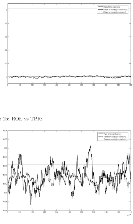
above unity and below 1. Indeed this is a Monetary Economy and claims

1 and 2 are veri…ed. It is also possible to prove that near the steady state

solution, the following holds: the return on equity of investors is the lowest in

this economy, followed by the return on money, which in turn is lower than

the return on equity of savers. All these rates of return are lower than the

rate of time preference, which is only surpassed by the marginal productivity

of capital9.

This ordering of interest rates plays a crucial role in this model and is a

direct consequence of having a monetary economy resulting from the liquidity

constraints. It is interesting to see that close to the steady state solution, not

only workers are discouraged from saving, because of too low rates of return,

but also savers lose from holding money and equity instead of consuming. It

is only because they face the possibility of having an investment opportunity

in the future that they decide to save: in such a situation they know that

they will need their own funds to …nance the downpayment of the investment

and allow them to produce the maximum possible amount of capital at a cost

lower than the price. It is worth emphasizing that investors want to invest,

not because their perceived return on capital is higher than their subjective

discount rate, but rather because capital sells at a price higher than its cost

(qt>1).

Notice that the wedge between the rates of return in this economy follows

exclusively from the fact that liquidity constraints are present. If there were no

liquidity constraints, funds would ‡ow from savers to investors until this wedge

had been shut down and capital price equaled its cost. However, because of this

…nancial friction, this economy will restrain the ‡ow of funds in a situation in

which investment is still in shortage, but no more funds are available to invest.

Consequently production stops below the First Best level.

The link between asset prices and business cycles lies in the precise fact that

shocks to the resaleability constraint have an impact on both the price of equity

and the amount of investment downpayment that investors are able to make. If

a liquidity shortage occurs ('_tsu¤ers a negative shock), the economy becomes more constrained and less funds will ‡ow from savers to investors. Investment

decreases and pulls capital accumulation downwards. Less capital stock results

in a lower real wage rate and in a higher gross pro…t rate (which is equal to the

marginal productivity of capital in this environment). Entrepreneurs will value

capital relatively more and consequently its price qt will rise. Facing lower

wages, workers decrease their consumption. As for entrepreneurs, even though

they increase their consumption on impact (due to their additional inability to

invest), as their net worth decreases in value they will necessarily decrease their

consumption level. In the end, investment, capital accumulation, consumption

and output will all break down and an economic recession kicks in. Clearly

there exists a feedback from the asset market on macroeconomic aggregates,

as the authors defend.

3 Neoclassical De-construction:

Above, I have summarized the model presented in KM. I am mainly interested

in understanding how this framework can be used to understand the e¤ects

proceed to calibrate and simulate this model, it is crucial to understand how

it works. For this purpose, in this section I start by simulating a standard

Neoclassical growth model and then proceed step by step, adding new

fea-tures to this basic framework until I end up with the KM economy. The …rst

step will be to review the simulation results obtained in the model by King

and Rebelo (1999), with the di¤erence that I will not include deterministic

technology growth in the model. Next, I will use a particular speci…cation

of the preferences in KM, i.e. the preferences in Greenwood, Herkowitz, and

Hu¤man (1988) - also referred to as GHH from this point onwards. In a third

step towards the KM model, I will introduce a distinction between two types

of agents in the economy. Finally, in Section 5, I will include the two …nancial

constraints presented above and allow for liquidity shocks. In each step I will

be checking for changes in volatility, comovement and persistence when

sto-chastic shocks are fed into the model and the simulation is performed. My goal

is to compare the ability of each model to replicate fundamental real business

cycles properties of the U.S. economy and to understand in which way the

liquidity constraints may bring about changes in the ability of Neoclassical

models to reproduce these RBC properties. In practice I will be deriving some

crucial RBC moments and comparing them with the corresponding statistics

1 synthesizes these statistics:

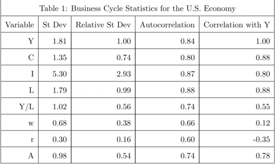
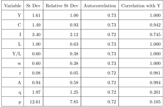
Table 1: Business Cycle Statistics for the U.S. Economy

Variable St Dev Relative St Dev Autocorrelation Correlation with Y

Y 1.81 1.00 0.84 1.00

C 1.35 0.74 0.80 0.88

I 5.30 2.93 0.87 0.80

L 1.79 0.99 0.88 0.88

Y/L 1.02 0.56 0.74 0.55

w 0.68 0.38 0.66 0.12

r 0.30 0.16 0.60 -0.35

A 0.98 0.54 0.74 0.78

Values in Table 1 are presented in log-deviations from the steady state and

in percentage terms.

3.1 Benchmark Neoclassical model:

In the paper by KR the authors consider a standard Neoclassical model in

which households have to choose a path for consumption, labour supply and

asset holdings. This problem can be described by:

M ax

fct;lt;at+1g

1 t=0

E0

1

X

t=0

t "

logct+

(1 lt)1 1 1

#

s:t: ct+at+1 (1 )at=wtlt+rtat

wherectis the consumption level,atis the amount of assets held andltstands

for labour supply. Households receive a rental rate r_t for the assets held and real wage wt for the hours worked. These are paid by competitive …rms that

and labour as inputs. The production function is a Cobb-Douglas:

yt=At(kt) (lt)1

where lt is the labour demand, kt is the stock of capital of each …rm and

At is an aggregate productivity coe¢cient. Since this is a closed economy

environment it results that at kt. This economy is hit by stochastic shocks

A_t that follows an AR(1) Markov process logA_t = _AlogA_{t 1} +"_A, where

"_A is an iid random variable with standard deviation A. Finally, contrary

to the case of KR, the model presented here is absent of growth. I perform

this modi…cation to the KR framework given that there is also no economic

deterministic growth going on in the KM framework. This very simple model

is then calibrated in such a way that some stylized facts for the U.S. economy

are met:

KR Model Calibration:

A A

0.984 3.48 0.333 0.025 1 0.979 0.0072

the model. These are presented in Table 2.

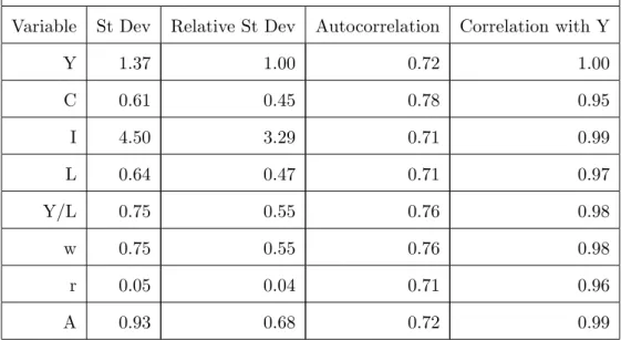
Table 2: Business Cycle Statistics for King and Rebelo RBC model

Variable St Dev Relative St Dev Autocorrelation Correlation with Y

Y 1.37 1.00 0.72 1.00

C 0.61 0.45 0.78 0.95

I 4.50 3.29 0.71 0.99

L 0.64 0.47 0.71 0.97

Y/L 0.75 0.55 0.76 0.98

w 0.75 0.55 0.76 0.98

r 0.05 0.04 0.71 0.96

A 0.93 0.68 0.72 0.99

The simulated shocks produce a model that is almost as volatile as the data

for the U.S. economy. In relative terms, consumption is two thirds smoother

than output and investment three times as volatile. Although consumption

lacks some volatility these results are more or less in line with the data. The

model fails though, in explaining the observed volatility in hours: the

sim-ulated standard deviation of 0:64% compares to the observed 1:79% in the U.S. data. Conversely, the real interest rate observed volatility of 0:30% is underestimated by the model which leaves this standard deviation at 0:05%. Persistence is reasonably well predicted by the model. Nevertheless,

underesti-mation is present in most variables and is particularly relevant for consumption

and output. On the contrary, both real prices are slightly more persistent in

the model than in the data. Finally, comovement comes with the right sign for

all variables but the real interest rate. Indeed, in Table 1 one can see that the

real interest rate is countercyclical in the U.S. economy, whereas in Table 2

is positive and close to one10_.

Moreover, in general, variables are too correlated with output when

com-pared with the data, particularly real wages, for which the observed correlation

coe¢cient is 0:12whereas the model predicts it to be of the order of 0:98. Despite the referred ‡aws, I use this model as a benchmark for a good

RBC simulation and compare it with the next simulations.

3.2 Neoclassical model with GHH preferences:

Consider now a slightly di¤erent Neoclassical Growth model where there is a

unit measure of in…nitely lived consumers with preferences:

E0

1

X

t=0

t_{U c} t

!

1 + (lt)

1+

where U(:) is increasing and strictly concave. Note that this formulation for preferences is the one present in KM. Following GHH, let the functional form

for the utility function be:

U(ct; lt) =

c_{t 1+}! (l_t)1+ 1 1 1

From this type of preferences one can derive the marginal utility of

con-sumptionUc(t) = _(c 1

t ₁₊! (lt)1+ ) and the marginal disutility of labourUl(t) = !lt

(ct 1+! (lt) 1+

) . The equilibrium conditions for households are:

lt=

wt

!

1

(39)

1 = Et "

(rt+ 1 )

ct ₁₊! (lt)1+

c_{t+1 1+}! (l_t+1)1+ ! #

(40)

As above, …rms equate the marginal utility of capital and labour to its

respec-1 0_{There is some debate, though, on whether the real interest rate is indeed countercyclical.}

tive rates of return:

rt= At

lt

kt

1

(41)

wt= (1 )At

kt

lt

(42)

Finally, the goods market clearing condition and the law of capital

accumula-tion are:

yt=At(kt) (lt)1 =ct+it (43)

it=kt+1 (1 )kt (44)

The above, together with the law of motion for the technology shocklogAt= AlogAt 1+"A, constitute the equilibrium conditions for this model.

Next, I proceed as above and calibrate the model so as to replicate some

stylized features of the U.S. economy. As in KR, I set = 0:984, so that the steady state annual interest rate equals 6:5%. Following the same paper, I choose the depreciation rate to be 10% per annum (which means that I

assume K_Y = 10 and _YI = 0:25). This leads to a quarterly gross depreciation rate 1 = 0:975. For the utility function parameters I set = 0:6 as in GHH, but choose a smaller value for the coe¢cient of risk aversion = 0:5

(rather than1:001as in GHH), to compensate for the inexistence of investment shocks in this model, contrary to the case in the GHH article. At last, with

this calibration in mind, I choose ! = 4:09, so that the average fraction of time spent working in the steady state equals 20%, as is commonly accepted

in the literature for the U.S. economy. The same technology shocks as above

are then performed and the resulting RBC moments are presented in Table 3.

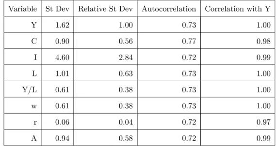
Consumption volatility increases at the expense of a lower investment

of output, while investment sees its variability slightly decreased to2:84 times the volatility of output, but still roughly in line with the data. A notable

improvement is made on the volatility of labour, which now accounts for63%

that of output. One last remark to the volatility of real wages which is now

exactly in line with the data. Almost no changes are noticeable in what

con-cerns persistence: as in King and Rebelo, this model still underestimates the

persistence of most variables (only real prices presidencies are overestimated).

Finally, comovement results are also similar to those in KR, even if they are

further away from the ones from the data.

Table 3: Business Cycle Statistics for a basic, GHH utility, RBC model

Variable St Dev Relative St Dev Autocorrelation Correlation with Y

Y 1.62 1.00 0.73 1.00

C 0.90 0.56 0.77 0.98

I 4.60 2.84 0.72 0.99

L 1.01 0.63 0.73 1.00

Y/L 0.61 0.38 0.73 1.00

w 0.61 0.38 0.73 1.00

r 0.06 0.04 0.72 0.97

A 0.94 0.58 0.72 0.99

One can therefore conclude that, changing the functional form of

pref-erences, does not signi…cantly interfere with the capacity of the Neoclassical

framework, to produce time series for the macroeconomic aggregates and prices

that perform reasonably well in predicting the observed volatility, persistence

and comovement in the U.S. data. Actually, despite the increased

overesti-mation of comovement, GHH preferences equip the Neoclassical model with a

better capacity to replicate the volatility in hours and consumption veri…ed in

3.3 Model with workers and capital owners:

In this section I introduce a distinction between two types of agents: workers

and capital owners. These play di¤erent roles in the economy, similarly to

what happens in KM, but without the …nancial constraints. As in KM, I

assume that workers want to consume all their labour income. This is an

absurd claim, given that nothing structurally prevents workers from wanting

to save and smooth consumption. Indeed, in this framework the rate of return

on capital equates the rate of time preference, thus providing an incentive for

workers to save. Nonetheless, I keep this assumption, on the grounds that it is

a step forward towards the model in KM. In practice, as we have already seen,

this claim is veri…ed in a neighborhood of the steady state in the model of KM,

provided that the liquidity constraints are stringent enough. In the end, this

fact will play a crucial role on the performance of the model to replicate the

U.S. real business cycles statistics and therefore is worth analyzing separately,

in the absence of liquidity constraints.

Assume there is a unit measure of both workers and capital owners.

Work-ers have preferences:

E₀

1

X

t=0

t c w

t 1+! (ltw)1+

1

1

1

as in the previous case, whereas capital owners have preferences of

consump-tion,ck_t:

E0

1

X

t=0

t_{log c}k t

and have access to a Cobb-Douglas production technologyyt=At(kt) ltk

1

,

where lk_t is the labour demand. With the output of their production, capital owners pay for labour, consume and invest in new capital. The ‡ow of funds

ck_t +kt+1 (1 )kt=At(kt) lkt

1

wtlkt

The Lagrangean for the problem of a representative capital-owner is:

L=E0

1

X

t=0

t_{log c}k t

+

1

X

t=0

E0 t At(kt) ltk

1

+ (1 )kt wtlkt ckt kt+1

Derive the …rst order conditions of the Lagrangean and work them out to

obtain the equilibrium conditions:

1

ck_t = Et

1

ck_t+1

yt+1

kt+1

+ 1 (45)

wt= (1 )At

kt

lk_t (46)

From the Euler Equation, (45), one can see that the gross pro…t, which I

de…ne asr_t, is equal to its marginal productivity:

rt=

yt

kt

(47)

As in the KM model, preferences are logarithmic and, therefore, the optimal

level of consumption for a representative capital owner is a fraction 1 of

his net worth. In this context, the net worth is the valuation of the capital

held by the agent at any given point in time, for a given rate of returnrtand

depreciation rate . Hence, consumption results in:

ck_t = (1 ) (r_t+ 1 )k_t (48)

labour:

cw_t =wtlwt (49)

The labour supply, instead, results from equating the marginal rate of

substi-tution to the real wage rate:

l_tw= wt

!

1

(50)

The aggregate conditions corresponding to expressions (45) to (50), together

with the goods market clearing condition Yt = Ctk+Ctw+It and the law of

motion for capitalIt=Kt+1 (1 )Kt, constitute the equilibrium conditions

for this economy.

I apply the same calibration to this model as the one in the model without

the distinction between workers and capital owners and produce the same

technology shocks. The RBC statistics for this model are presented in Table

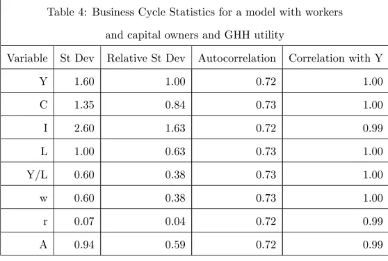
4. Comparing the simulation moments of this model with the ones presented

in Table 3, we can conclude that, intuitively, non-optimizing workers lead to a

much greater consumption volatility than before - it now accounts for almost

85% of the output’s standard deviation -, investment loses a great amount

of variability - it is now only 1:63 times as volatile as output - and all other variables keep approximately the same standard deviation. In what concerns

to the ones resulting from the previous model.

Table 4: Business Cycle Statistics for a model with workers

and capital owners and GHH utility

Variable St Dev Relative St Dev Autocorrelation Correlation with Y

Y 1.60 1.00 0.72 1.00

C 1.35 0.84 0.73 1.00

I 2.60 1.63 0.72 0.99

L 1.00 0.63 0.73 1.00

Y/L 0.60 0.38 0.73 1.00

w 0.60 0.38 0.73 1.00

r 0.07 0.04 0.72 0.99

A 0.94 0.59 0.72 0.99

Hence, when one distinguishes between workers and capital owners and

forces the …rst to consume their entire labour income, the model performance

in predicting the RBC features of the U.S. economy changes considerably. This

results from the fact that consumption and investment volatility, respectively,

increase and decrease signi…cantly. This comes at no surprise, given that, by

inhibiting workers from saving, I am depriving a proportion of agents from the

ability to smooth consumption. In boom times, consumption from workers is

too high and funds that would otherwise be used for investment are consumed.

Conversely, during recession periods, workers consume too little, given that

they do not dispose of any savings to smooth their behavior. This fact will

play a crucial role in the simulation of the model by Kiyotaki and Moore, in

which case the claim that workers consume their labour income is legitimated

by the fact that liquidity constraints indeed prevent workers from wanting to

4 Calibration:

Before I take the …nal step and perform the dynamic analysis and simulation of

the model in KM, I must go through the details of the calibration. As before,

I am calibrating this economy assuming that each period represents a quarter.

First, following KR, assume that the capital-output ratio is K_Y = 10and that

the investment-capital ratio is _YI = 0:25. These lead to a quarterly gross rate of depreciation = 1 _K=YI=Y = 0:975. In what concerns the elasticity of labour supply, I set = 0:6as described above. Note that in the a First Best solution, with no …nancial constraints, the gross pro…t rate (or the marginal productivity

of capital) is equal to the rate of time preference. Such equilibrium is one of the

possible outcomes of the current model - one in which the liquidity constraints

are set to = ' = 1 and the gross pro…t rate rt corresponds to the real

interest rate - hence, I use this result to calibrate the discount factor : again,

following KR set the real interest rate at 6:5% per annum in the First Best scenario, which implies that is set to 0:984on a quarterly basis. With this calibration in mind, I choose a value for ! that guarantees that the average fraction of time spent working in the steady state equilibrium equals 20%, as

is commonly accepted in the literature for the U.S. economy.

My aim is to calibrate this economy in such a way that the level of q

resulting from the steady state equilibrium is in line with the average q for the U.S. economy, as estimated in Laitner and Stolyarov (2003) - LS in what

follows. In this article the authors use U.S. annual investment data from 1953

to 2001 in order to estimate a time series forq. According to their study, the level ofq averaged1:2075during their period of analysis. I consider this to be the steady state level for q and calibrate the …nancial constraints accordingly. Consider the resaleability constraint …rst. It is not straightforward to …nd

an empirical support for this type of …nancial restriction. However, a detailed

pre-sented in Negro, Eggertsson, Ferrero and Kiyotaki (2009) - henceforth, NEFK

- and used to match the same resaleability constraint. I follow this article

in order to calibrate the stochastic liquidity shock. I construct an historical

series from 1952jQ1 to 2008jQ4 for the liquidity share in the U.S. as de…ned

in NEFK: LS_t = ptMt

ptMt+qtKt. From this data I extract the average liquidity

share and its autocorrelation and standard deviation coe¢cients. These are

given by '_ss = 0:11, _' = 0:969 and ' = 0:029 and provide an estimation

for steady state level of 'and for its law of motion, when calibrated for the U.S. economy11_{. In what concerns the borrowing constraint I choose so that}

the leverage ratio in this economy is in line with the observed average

debt-to-equity ratio of four in the U.S. economy - in line with Gertler and Kiyotaki

(2009). For each unit of investment, an entrepreneur borrows an amount q

from savers and …nances1 q with her own funds. Hence I set:

4 = q

1 q

) t66:3%

I am left with the investment opportunity arrival rate to calibrate. Since

there is no obvious direct evidence for this rate, I choose the value of in

such a way that the level of q resulting from the steady state equilibrium in this economy is given byq = 1:2075, in line with LS, as previously referred12. Such calibration implies that each quarter an entrepreneur has a probability

1 1_{Notice that, although'}

tis de…ned as the rate at which an entrepreneur can alienate her old equity holdings, in order to fund her investment opportunity (i.e. as a ‡ow variable), hereby I am tracking it with a picture of how liquid an economy is on average (i.e. as a stock variable). Clearly the stock of liquidity in a given economy is intrinsically related with the velocity with which one is converting the illiquid asset (equity) into the liquid one (money). Following NEFK, I argue that, on average, the velocity at which equity is exchanged for money equates the aggregate liquidity share.

1 2_{In Negro, Eggertsson, Ferrero and Kiyotaki (2009), the authors directly calibrate the}

investment opportunities arrival rate at 7% per quarter. They argue that this value is probably an upper bound for this coe¢cient.

of approximately1:82% of facing an investment opportunity.

The calibration of this model is summarized in the following table:

KM Model Calibration:

! '

0.984 0.6 0.975 4.67 0.663 0.11 0.018

In what concerns the stochastic technology coe¢cientA_tit is easy to choose a law motion: following KR, simply set _A = 0:0979 and A = 0:0072 as I

have already done for the simpli…ed Neoclassical models presented above.

5 Dynamics:

In this section I analyze the behavior of the macroeconomic aggregates and

prices in the model by KM, when hit by shocks in the stochastic variables.

Although the model of KM incorporates only two stochastic variables (Atand

'_t), I treat an extra couple of parameters as such, in order to understand how the model reacts to sudden changes in both the arrival rate of investment

and in the borrowing constraint .

I start with a shock to the productivity variable A_t and suppose that its law of motion is given bylog (At) = _Alog (At 1)+"At, where the error term"At

is theiid technology shock. I am interested in analyzing the impulse response

functions of prices and aggregates to unexpected changes in the technology

coe¢cient. Following the above described calibration, I set _A = 0:979 and I consider a1% shock toAt. The impulse response functions for this shock are

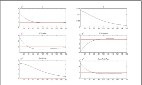
presented in Figures 2a and 2b in appendix.

When the productivity shock hits the economy, the marginal productivity

increases and departs further from the rate of time preference. This means

that the economy becomes virtually more constrained: each unit of investment

respond and drive its marginal productivity downwards until the subjective

discount rate was reached. In this setup, though, capital production is

con-strained, which means that an increase in the marginal productivity of capital

boosts its value and leads to an increase in its priceq_t. A higher equity price decreases the downpayment required per unit of investment. Hence,

invest-ment increases and pushes capital accumulation upwards. Given that money

is an input for investment, the increase in qt drives the price of money pt

up-wards. The upward reaction in both prices and in the productivity of capital,

in turn, increases the value of entrepreneurs’ net worth, this way fuelling the

rise in investment and consumption. In the mean time, a higher capital stock

leads to an increase in the real wage rate, which results in a higher

consump-tion level of workers. Entrepreneurs, however, will consume less on impact,

due to the increased attractiveness of investment that constitutes a strong

sub-stitution e¤ect. On aggregate, consumption starts by responding downwards,

only to increase as the shock vanishes and output expands, allowing for the

income e¤ect to exceed the substitution e¤ect.

From the above we can conclude that this model includes an ampli…cation

e¤ect. Note that, after the liquidity shock, investment jumps in response to

the rise in the marginal productivity of capital, as usual. However, as prices

rise in response to the higher value of capital, the net worth of entrepreneurs

increases in value, providing more funds for investment. Furthermore, also the

required downpayment1 q_tdecreases as the price of capital rises, providing an additional source of investment growth.

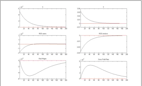
Consider a persistent negative shock to the resaleability constraint. As

de…ned in Section 4, '_t follows an AR(1) Markov process that is stationary around '_ss = 0:11. Thus we have '_t = 1 _' '_ss + _''_{t 1} +"'_t where

shock to '. Following the calibration in Section 4 set _' = 0:969. As for the scale of the shock I consider a liquidity deterioration in which'_t decreases by

1p:p:.

When'_tdecreases investors see their ability to raise funds, out of their pre-viously held equity, reduced. The amount of equity converted into investment

funds decreases, meaning that investment decelerates and capital

accumula-tion drops, pushing its marginal productivity upwards. In what concerns the

price of equity, two contradictory forces are at place. On the one hand, equity

is now less desirable, given that is relatively less liquid than before.

Entrepre-neurs perform a so called ‡ight to quality and demand more money and less

equity, this way driving the price of equityqtdownwards. On the other hand

though, and most importantly, capital is now scarcer and its marginal

pro-ductivity higher. This means that each unit of equity used by entrepreneurs

for investment is now more valuable, and this ultimately pushes the price of

equity qt upwards. We can see from Figure 3b that, in the end, this second

e¤ect prevails and qt raises in response to a negative shock to't. Intuitively,

since we are further departing from a situation where there is no resaleability

constraint on equity and where the price of capital equals its cost(qt= 1), it

be…ts naturally that a sudden reduction in liquidity drives the price of capital

upwards. The higher demand for money resulting from the ‡ight to quality,

together with the increased value of investment, both lead to an increase in

its pricep_t. As for consumption, it will be driven upwards on impact, due to the substitution e¤ect created by the increased funding di¢culties. However,

as capital accumulation freezes and investment slows down, output falls and

inevitably consumption is pushed downwards. Note that consumption of each

type of agent reacts di¤erently: while entrepreneurs decide to consume more

on impact, only to decrease their consumption as output slows down, workers

Interestingly, in the case of a stochastic shock to liquidity, this model

im-plies a absorption rather than an ampli…cation e¤ect. In fact, as the

resaleabil-ity shock hits the economy, investment breaks and leads capital accumulation,

consumption and output downwards. However, as asset prices react positively,

entrepreneurs’ pain is relieved by an increase in their net worth value, which,

in turn, cushions the drop in the macroeconomic aggregates.

It is clear from this analysis that a liquidity shock can qualitatively

repro-duce an economic recession like the one the world economy has been facing

since the summer of 2007. Furthermore, it is interesting to see that even a

transitory shock to '_t can produce a long-lived recession: if we set _' = 0

and simulate the same liquidity shock as above, it can be seen from Figure 3c

and Figure 3d that, although prices and investment swiftly return to normal

as the shock vanishes, capital accumulation, consumption, output, real wages

and the gross pro…t rate take a lot longer to retrieve to their steady state level.

If, instead, we consider a shock to the borrowing constraint coe¢cient ,

very similar qualitative results are obtained. Assume that, tfollows anAR(1)

Markov process: t= (1 ) ss+ t 1+"t. In Section 4 I have calibrated

the steady state borrowing constraint parameter ss = 0:663, but not the

persistence or scale of its shock, given that is set constant in KM. As I am

only interested in checking for the qualitative impact of a persistent shock

to the borrowing constraint, I take a shortcut and use the same persistence

coe¢cient as I did with the resaleability constraint: = 0:969. The graphics for the impulse response functions of a sudden decrease of one 1p:p:in t, are

depicted in …gures 4a and 4b.

When t decreases, a higher downpayment will be required per unit of

investment. Investors will, suddenly, be incapable of leveraging as much output

claims as they did before. Hence, the ability of investors to issue inside equity

of liquidity. Aggregate investment decreases due to the shortage of funds and

along with it capital accumulation decelerates. For lower levels of capital

stock, the marginal productivity of capital rt rises. As with the shock to 't,

the price of equity su¤ers two distinct e¤ects: the …rst one pushes q_t upwards and results from the increased value of capital (income e¤ect), whereas the

second one drives qt downwards and results from the entrepreneurs’ portfolio

adjustment (substitution e¤ect). In the end the income e¤ect prevails and qt

responds upwards. As before, the price of money pt is driven upwards by the

adjustment in the portfolio composition and the increased value of investment.

Finally, like with the shock to ', aggregate consumption responds positively at …rst, but eventually starts to decrease as the income e¤ect surpasses the

substitution e¤ect.

One can therefore conclude, that a reduction in the pledgeable fraction

of investment leads to the same qualitative results produced by a contraction

in the resaleability of equity, even though the triggering shock is structurally

di¤erent: in fact, a shock to t has an impact directly on the downpayment

of investment and constitutes a shock to the leveraging ability of investors; a

shock to '_t, instead, decreases the ability of investors to resell their equity, with only indirect e¤ects on the required downpayment.

Finally, consider a persistent shock in the arrival rate of investment

op-portunities . The impulse response functions of macroeconomic aggregates

and prices, with respect to a 1p:p: increase in , are plotted in …gures 5a and 5b respectively. De…ne t as an AR(1) Markov process that is

station-ary around some steady state which I denote as ss. This way one can write

t= (1 ) ss+ t 1+"t where"t is aniid shock. Recall that there is

no aim at correctly microfounding the arrival rate of investment opportunities.

Instead, I choose a calibration procedure that forces this economy to be in a

For this reason, I pick ss = 0:018 and simply set the persistence coe¢cient

to be = 0:95, so that we can capture the e¤ects of a persistent decrease in the investment opportunities arrival rate. I study the impact of a rise in t of

one percentage point.

In order to understand the qualitative impact of a shock to t, it is useful

to think about an extreme situation in which entrepreneurs face an investment

opportunity with probability one ( = 1): in such case, investment

opportu-nities are useless, given that, although every entrepreneur wants to sell equity

claims, there is no demand for them, for the simple reason that savers have

been extinguished. The only logical equilibrium in such situation is to have

qt = 1and pt = 0, which means that investors are indi¤erent between

invest-ing and savinvest-ing, and money, as a consequence, plays no role in this economy.

Therefore, if one considers a positive shock that departs from ss, it is only

reasonable to expect that when the arrival rate of investment opportunities

rises, prices of both assets should fall. From the equilibrium conditions, it

can be seen that a rise in t leads to an increase in the aggregate investment

that is independent of the downpayment required per unit of output invested:

investment rises simply because there are more people investing. Capital

accu-mulation necessarily soars and, in the mean time, consumption breaks down,

given that there is now a larger fraction of agents in the economy who have

access to investment and thus value consumption relatively less.

In a sense, a positive shock to t increases the ability of this economy

to avoid the liquidity constraint. Liquidity is the more important the more

infrequent are investment opportunities. The main reason for this to happen

hinges on the fact that with a lower fraction of savers in the economy, there

are less funds to be transferred from savers to investors and, therefore, the

restringency in the ‡ow of these funds (i.e. the liquidity constraint) loses