State-of-Charge for Battery Management System via Kalman Filter

State-of-Charge for Battery Management System

via Kalman Filter

T. O. Ting, Ka Lok Man, Chi-Un Lei, Chao Lu

Abstract—Battery Management System (BMS) requires an indefinite accurate model. With an aging model, the lifetime of a battery can be precisely predicted with respect to the State-of-Charge (SoC) of a battery. The mathematical model in terms of state variables involving smart BMS is presented in this work. The state space model is crucial as an accurate model and is able to represent the complex dynamic behavior of a battery system. A numerical case study is done to verify the model obtained through mathematical derivations by adopting the prominent RC battery model from literature. Furthermore, the well-known Kalman filter (KF) is applied to estimate the SoC of a battery system. With accurate prediction of SoC of battery system, its lifetime could be prolonged, and thereby saving us substantial cost.

Index Terms—Battery Management System (BMS), battery modeling, Kalman filter, State-of-Charge, state space.

I. INTRODUCTION

T

HE understanding of a battery system is essential before efficient management system could be designed [1], [2], [3]. Hence, a generic tool to describe the battery performance under a wide variety of conditions and applications is highly desirable [1]. As such, the electrical modeling is able to provide such a tool that enables visualization of the processes occurring inside rechargeable batteries. Only with the pres-ence of these generic models could new battery management system be developed for reliable performance. These algo-rithms control the operation and maintain the performance of battery packs. The ultimate aim is to prolong battery life and ensures reliable safety alongside many applications, especially in photovoltaic systems [4], [5], [6].

Battery modeling is done in many ways depending on the types of battery. In general, the resulted battery model is mathematical model comprising of numerous mathematical descriptions [7]. Ultimately, the battery models aim to deter-mine State-of-Charge (SoC) of a battery system. However, the complexity of the nonlinear electrochemical processes has been a great barrier to modeling this dynamic process accurately. The accurate determination of SoC will enable the utilization of battery for optimal performance, long lifetime, and prevent irreversible physical damage to the battery [8]. Solutions to SoC via neural networks [9] and fuzzy logic [10] have been difficult and costly for online implementation due to large computation, causing the battery pack controller to

Manuscript received April 22, 2014; revised May 1, 2014. This work was supported by Xi’an Jiaotong-Liverpool University under RDF-13-01-13.

T. O. Ting is with the Department of Electrical and Electronic Engineer-ing, Xian Jiaotong-Liverpool University, China. Email: toting@xjtlu.edu.cn K. L. Man is with the Department of Computer Science and Software Engineering, Xian Jiaotong-Liverpool University, China and Department of Computer Science, Yonsei University, Korea. Email: ka.man@xjtlu.edu.cn

C.-U. Lei is with the Department of Electrical and Electronic Engineering, The University of Hong Kong, Hong Kong. Email: culei@eee.hku.hk

C. Lu is with Purdue University, West Lafayette, Indiana. Email: eeluchao@gmail.com

be heavily loaded. However, this can be a good alternative in the near future due to the increased computational power of processing chips alongside their declining cost.

Model-based state-estimation has been proposed in [11], [12], [13]. In [12] a state-estimation model had been utilized for the determination of optimized charging current using Genetic Algorithm (GA). In [14] Ant Colony algorithm was applied to determine the charging current in each stage to reduce charging time. In control theories, the well-known Kalman filter [15] had been applied successfully for both state observation and prediction problems [11]. Work in [16] utilized manufacturers’ data in modeling the dynamic behavior of battery.

In this work, a mathematical derivation leading to a state space model is presented. The basic schematic model is adopted from [11], [13]. Hereby, a thorough analysis in the form of state variables with the application of Kalman filter is presented. The rest of the paper is organized as follows. Section II discusses the factors of battery aging. A mathematical model is derived in Section III, describing the state space model. Results are presented in Section V, and finally the conclusions are derived in Section VI.

II. BATTERYAGING

Identification of key aging parameters in battery models can validate degradation hypotheses and provide a foundation for estimation of battery status, e.g. State of Health (SOH). In brief, aging and degradation of batteries can be caused by capacity fading (the loss of battery charging/discharging capacity over time) as well as power fading (the loss of absorbing and delivering electrical power). From another perspective, power fading and energy fading are associated with impedance rise and capacity loss, respectively. Detailed discussion of typical aging effects can be found in [17]. A few major effects are outlined in the following subsections.

A. Thermal Degradation

bThe performance of a battery is significantly affected by temperature. For instance, Lithium battery can effectively operate between −30◦_{C and 52}◦_{C. When the temperature}

drops below −30◦_{C, diffusion and chemical reactions}

be-come inactive and thus battery impedance increases dramat-ically. On the other hand, when the temperature rises above 60◦_{C, the battery has a significant capacity loss. Also, if the}

temperature rises above85◦_{C, the battery could be damaged}

B. Physical Damage

Battery aging can also be caused by electrode fracture and fatigue. In existing literatures, a specific electrode model and a diffusion-induced stress model have been proposed for in-vestigation [18]. Results showed that the output voltage does not change significantly, however it increasingly accumulates stress.

C. Particles Accumulation

Solid Electrolyte Interphase (SEI) is formed on the surface of electrodes when the battery is charged, and in particular, when electrode starts to react with the electrolyte. SEI ab-sorbs mobilized Lithium ions and slows down the transporta-tion of ions between electrode and electrolyte. These form crystalline introduce power fading and capacity fading. In the case of low and high current densities, moss and dendrite are formed on the surface of negative electrode. These substances reduce surface area of electrodes for reactions, and thus causing battery fading.

D. Aging Characterization

Measurements are needed in order to accurately char-acterize aging in batteries. To investigate the cycle life capabilities of lithium ion battery cells during fast charging, cycle life tests have been carried out at different constant charge current rates. Through measurement results, cycle life models have been developed to predict the battery cycle ability. The analysis indicates that the cycle life of the battery degrades when the charge current rate increases. In addition, the measurement of battery impedance via electrochemical impedance spectroscopy (EIS) and the current-pulse tech-nique [19] helps in determining battery health.

In order to ensure a uniform temperature during battery operations, maintaining battery performance, and eventually prolong the battery lifetime, real-time temperature sensing and monitoring systems as well as cooling systems are needed [20], [21], [22]. In addition, in order to improve cycle stability and battery capacity, thick anodes (e.g. about 1 mm) are adopted for Li-ion batteries. These anodes consist of vertically aligned carbon nanotubes which are coated with silicon and carbon [23].

E. Aging Models

Aging parameters in Lithium-ion batteries vary with dif-ferent current rates, working temperatures and depths of discharge. For example, in order to model the thermal characteristics of the battery that causes battery aging, it is necessary to model the generation of heat inside the battery, heat transfer between battery and the environment, and the reactivity of chemical reactions with respect to the temperature [24]. In particular, in order to correctly model the thermal distribution and characteristics of battery packs, lumped thermal models are formulated to model the ohmic heating in battery cell packs [25]. The aging parameters can be applied for early aging detection. Through early detection and appropriate maintenance, performance of battery cells can be significantly improved. Detection can be done by analyzing real-time data from operations of batteries (e.g. voltage and current data from lithium-ion cells). In [12],

!"

!# !$

%#&'()*$ %+, !"# !"$

-# -+

./

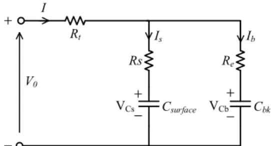
-Fig. 1. Schematic ofRCbattery model

battery aging detection is done based on the sequential clustering of battery packs. During operations, a derived fuzzy model is used to predict operation performance and detect the aged battery via similarity comparisons, with respect to the ideal situation.

III. BATTERYMODEL[13]

Several battery models existed over the past years. Each of these models varies in term of its complexity and appli-cations. In this work, a dynamical battery model is adopted, consisting of state variable equations, from [11], [13]. The schematic representation of this model is shown in Fig. 1. In this model, there exists a bulk capacitor Cbk that acts as a energy storage component in the form of charge, a capacitor that models the surface capacitance and diffusion effects within the cell Csurf ace, a terminal resistance Rt, surface resistance Rs, and end resistance Re. The voltages across both capacitors are denoted asVCbandVCs, respectively.

A. Mathematical Derivations of Battery Model

In this derivation, we aim to form a state-space model consisting of the state variables VCb, VCs and V0. State

variables are mathematical description of the ”state” of a dynamic system. In practice, the state of a system is used to determine its future behaviour. Models that consist of paired first-order differential equations are in state-variable form.

Following the voltages and currents illustrated in Fig. 1, the terminal voltageV0 can be expressed as

V0=IRt+IbRe+VCb, (1)

which is similar to

V0=IRt+IbRs+VCs. (2)

By equating the (1) and (2), and after simple algebraic manipulation, which results in

IbRe=IsRs+VCs−VCb. (3)

From Kirchoff’s laws,I=Ib+Is,

Is=I−Ib, (4)

Substituting (4) into (3) yields

Ib(Re+Rs) =IRs+VCs−VCb. (5)

By assuming a slow varyingCbk, that isIb=CbkV˙Cb(from basic formula of i = C∂V

˙

VCb=

IRs

Cbk(Re+Rs)

+ VCs

Cbk(Re+Rs)

− VCb

Cbk(Re+Rs)

. (6)

By applying a similar derivation, the rate of change of the surface capacitor voltage, derived also from (1) and (2) as

˙

VCs=

IRe

Csurf ace(Re+Rs)

− VCs

Csurf ace(Re+Rs)

+ VCb

Csurf ace(Re+Rs)

. (7)

By assuming A = 1

Cbk(Re+Rs) and B =

1

Csurf ace(Re+Rs),

(6) and (7) can be written as

˙

VCb=A·IRs+A·VCs−A·VCb, (8)

and

˙

VCs=B·IRe−B·VCs+B·VCb, (9)

respectively. Further, (8) and (9) can be combined to form a state variable relating voltages VCs and VCb and current flow I, which is

_˙ VCb ˙ VCs =

−A A

B −B

VCb

VCs

+

A·Rs

B·Re

I. (10)

Next, the output voltage is derived from (1) and (2). By adding both equations, we obtain

2V0= 2IRt+IbRe+IsRs+VCb+VCs. (11)

By substitutingIb=_RsR₊s_Re andIs= _RsR₊e_Re into (11), it is further simplified as

V0=

VCb+VCs

2 +

Rt+

ReRs

Re+Rs

I (12)

By taking the time derivative of the output voltage and assuming dI/dt ≈ 0 (this simply mean that the change rate of terminal current can be ignored when implemented digitally). Hence we get

˙

V0=

˙

VCb+ ˙VCs

2 . (13)

By substituting the values obtained earlier in (8) and (9) into (13), results in

2 ˙V0= (−A+B)VCb+ (A−B)VCs+ (ARs+BRe)I. (14)

Then, by solving forVCs from (12) we obtain

VCs= 2V0−2(Rt+

ReRs

Re+Rs

)I−VCb, (15)

and after substitution into (14) yields

˙

V0= (−A+B)VCb+ (A−B)V0

+ [A(0.5Rs+Rt+D) +B(0.5Re−Rt−D)]I. (16)

Finally, the complete state variable network is obtained by integrating (16) into (10), thus the complete state variable description of the network is obtained as

  ˙ VCb ˙ VCs ˙ V0  =  

−A A 0

B −B 0

(−A+B) 0 (A−B)  ·   VCb VCs V0  +  

A·Rs

B·Re

A(0.5Rs−Rt−D) +B(0.5Re+Rt+D) 

I, (17)

whereby constantsA,B andD have been given earlier and hereby restated as

  A B D  =    1

Cbk(Re+Rs)

1

Csurf ace(Re+Rs) ReRs Re+Rs





. (18)

This completes the initial derivation of a battery model.

B. Numerical Example

By substituting all capacitor and resistor values from Table I into (18), we obtain relevant values as

  A B D  =   0.001508759347566 1.623837940973491 0.001875000000000 

. (19)

By defining matrixM,

M=





−A A 0

B −B 0

(−A+B) 0 (A−B) 

, (20)

and

N=





A·Rs

B·Re

A(0.5Rs−Rt−D) +B(0.5Re+Rt+D) 

,

(21) again by substituting all the values from Table I and calcu-latedA, B andD, we obtain the value ofM as

M=





−1.51×10−3 _1.51×10−3 ₀

1.6238 −1.6238 0

1.6223 0 −1.6223



, (22)

andNas

N=





5.66×10−6

6.08×10−3

1.05×10−2



. (23)

As such (17) can be rewritten as

  ˙ VCb ˙ VCs ˙ V0 

=M·   VCb VCs V0 

+N·I, (24)

or numerically as

  ˙ VCb ˙ VCs ˙ V0  =  

−0.0015 0.0015 0 1.6238 −1.6238 0

1.6223 0 −1.6223

 ·   VCb VCs V0  +  

5.66×10−6

6.08×10−3

1.05×10−2



Step Response

Time (seconds)

Amplitude

0 20 40 60 80 100 120

0 1 2 3 4 5 6 7 8x 10

−3

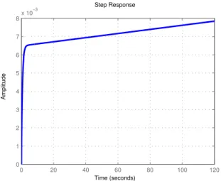
Fig. 2. Output response of RC model due to constant input.

C. State Space Modeling

Based on control theories, a lumped linear network can be written in the form

˙

x(t) =Ax(t) +Bu(t),

y(t) =Cx(t) +Du(t). (26)

where in this work, the state variablex(t)˙ is

˙ x(t) =



 ˙

VCb

˙

VCs

˙

V0



. (27)

Obviously,

x(t) = 



VCb

VCs

V0



, (28)

with

u(t) =I, (29)

and the outputy(t)is given as

y(t) =V0. (30)

This means that the output of the system is the open terminal voltage that we wanted, as expected. Also, by comparing (37) and (24) , it is easily noted thatA=M, that is

A=





−1.51×10−3 _1.51×10−3 ₀

1.6238 −1.6238 0

1.6223 0 −1.6223



, (31)

andB=N, which is

B=





5.66×10−6

6.08×10−3

1.05×10−2



, (32)

while

C=

0 0 1

, (33)

and the last one,

D=

0

. (34)

Further, the above state space variables are transformed to a transfer function, G(s). This is done by using ss2tf function in Matlab, and thereby, after factorization yielding

G(s) = 0.01054s

2_{+ 0.0171s+ 2.981×10}−5

s3_{+ 3.248s}2_{+ 2.637s−1.144×10}−18 (35)

The plot of the unit step response for the gain in (35) is given in Fig. 2. Basically, it shows that the open circuit terminal voltage V0 in Fig. 1 increases linearly during charging

operation in a very slow manner after transient behaviour for a few seconds.

TABLE I

PARAMETERS FORCELLMODEL[11], [13]

Cbk Csurf ace Re Rs Rt 88372.83F 82.11F 0.00375Ω 0.00375Ω 0.002745Ω

D. Observability of the RC Battery Model

In control theory, observability is a degree in predicting the internal states of a system via its external outputs. As such, for an observable system, the behaviour of the entire system can be predicted via the system’s outputs. On the other hand, if a system is not observable, the current values of some of its states cannot be estimated through output signal. This means that the controller does not know the states’ values. In theory, the observability of a system can be determined by constructing observability matrixOb.

Ob=



     

C CA CA2

.. .

CAn−1



      ,

and a system is said to be observable if the row rank ofOb is equal to n (this is also known as full rank matrix). The ultimate rationale of such test is that if nrows are linearly independent, then each of the n states is viewable through linear combinations of the outputy(t).

Further, by substituting allA, B, C and D values from (31)-(34), we obtain

Ob=





0 0 1

1.6223 0 −1.6223

−2.6344 0.0024 2.6320 

. (36)

Clearly, in this caseObis a full rank matrix, which concludes that this system is observable.

IV. KALMAN FILTER FORSOC ESTIMATION

As given in (??), a continuous time-invariant linear system can be described in state variable form as

˙

x(t) =Ax(t) +Bu(t),

y(t) =Cx(t). (37)

where

u input vector, x is the state vector, y is the output vector,

A is the time invariant dynamic matrix,

B is the time invariant input matrix,

C is the time invariant measurement matrix.

x(n+ 1) =Ad·x(n) +Bd·u(n)

y(n+ 1) =Cd·x(n+ 1) (38)

where

Ad≈I+A·Tc, Bd=B·Tc, Cd=C, (39)

whereIis the identity matrix andTcis the sampling period. As for this system, two noises are present which are additive Gaussian noise,

w vector representing system disturbances and model inaccuracies, and

v vector representing the effects of measurement noise.

Bothw andvhave a mean value of zero and the following covariance matrices

E[w·wT] =Q,

E[v·vT] =R, (40)

where E denotes the expectation (or mean) operator and superscriptT means the transpose of the respective vectors. In usual case,QandRare normally set to a constant before simulation; in our case both are set to one (see Section V). By inclusion of these noises, the resulting system is now can be described by

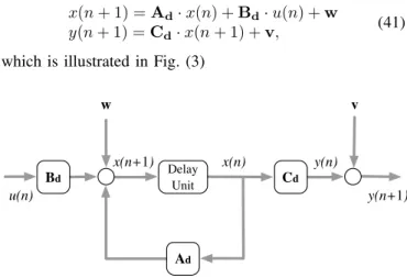
x(n+ 1) =Ad·x(n) +Bd·u(n) +w

y(n+ 1) =Cd·x(n+ 1) +v, (41)

which is illustrated in Fig. (3)

Bd Delay

Unit Cd

w v

y(n+1)

y(n) x(n)

x(n+1)

u(n)

Ad

Fig. 3. Discrete system model with noiseswandv

A. Property of Kalman filter

An important property of Kalman filter (KF) is that it minimizes the sum-of-squared errors between the actual valuexand estimated statesxˆ, given as

fmin(x) =E [x−x]ˆ ·[x−x]ˆT (42)

To understand the operations of KF, the meaning of the notationx(mˆ |n)is crucial. It simply means that the estimate ofxat eventmtakes into account all the discrete events up to eventn. As such, (43) can include such information, now expanded as

fmin(x) =E [x(n)−ˆx(n|n)]·[x(n)−x(nˆ |n)]T

(43)

In recursive implementation of KF, the current estimate ˆ

x(n|n), together with the input u(n) and measurement signalsy(n)are used for further estimating x(nˆ + 1|n+ 1).

B. KF Online Implementation

In the case of battery, it is well understood that only the terminal quantities can be measured (terminal voltage V0

and current I). Assuming that battery parameters are time-invariant quantities, the recursive KF algorithm is applied. By applying (39) into (31)-(33), we obtain the following updated matrices, withTc= 1:

Ad=





0.9984 1.51×10−3 ₀

1.6238 0.6238 0

1.6223 0 0.6223



,

Bd=





5.66×10−6

6.08×10−3

1.05×10−2



, (44)

Cd=

0 0 1 .

Note thatBdandCd remain similar to its previous values, as given in (32) and (33).

V. RESULTS

The program, implemented in Matlab language is given in Appendix A to clarify the results obtained in this work. The output of the program is given as Appendix B, hereby shorten to save printing page. Some important results obtained in this work are available in this part. Note that Q and R

mentioned in (40) are both set to one. The results obtained are tabulated in Table II. From these results, the Root-Mean-Squared (RMS) of the estimated error, which is the error from Kalman filter is far smaller compared to the measured error, with values of1.0013V and1.92×10−4_V

respectively. The time plot of this error from 0s to 60000s is shown in Fig. 4, depicting very small amplitude (≈0.04 V) along the timeline.

TABLE II RECORDEDRMS ERROR

RMS Error Value

Measurement,y−y_v 1.00136010496 Estimated (KF),y−_ye 1_.91859×10−4

0 1 2 3 4 5 6

x 104 −0.06

−0.04 −0.02 0 0.02 0.04 0.06

time (s)

Error

A. Charging Behaviour

The charging characteristic is illustrated in Fig. 5 whereby the initial terminal voltage V0 starts from 0 V up to

approximately 1 V (1.045 V to be exact) within 60000 seconds (which is 100 minutes). This, as expected, is a time consuming process as in usual case it may take hours for an aqueous battery (lead acid) to be completely charged.

0 1 2 3 4 5 6 x 104 0

0.2 0.4 0.6 0.8 1 1.2 1.4

time (s)

Cell terminal Votage (V

o

)

Fig. 5. Dynamic behavior of KF estimator with charge constant current of 1.53 A.

B. Discharging

For discharging process, the initial value of terminal voltage, y0 = V0 is set to 2.2 V in the Matlab program.

The dynamic behaviour showing the discharge characteristic is shown in Fig. 6. From this figure, it is observed that the discharge process is similar to charging; but now with linearly decreasingV0 slope. The open terminal voltage V0

drops from 2.2 V to 1.2 V in 60000 seconds (100 minutes); this is similar to the charging process as it literally takes 100 minutes to reachV0= 1V from zero potential.

0 1 2 3 4 5 6 x 104 1

1.5 2 2.5

time (s)

Cell terminal Votage (V

o

)

Fig. 6. Dynamic behavior of KF estimator with discharge constant current of -1.53 A.

VI. CONCLUSION

In this work, the factors of battery aging are discussed in details. Subsequently, we successfully obtain the state variables of the RC model that represents a battery in terms of mathematical derivations. The derivations come to a conclusion that there exists four state variables relevant to battery model. Further, based on control theories, we successfully plotted the response of the system, depicting a linearly increasing characteristic. With this state-estimation model, a prominent technique known as Kalman filter is applied with the aim of estimating State-of-Charge of Battery Management System. From numerical results, KF is more accurate in predicting the dynamic. This is shown by very small RMS error of the estimated error in comparision to its measurement error.

ACKNOWLEDGMENT

We appreciate the generosity of our colleagues, Nan Zhang and Sanghyuk Lee in sharing their expertise knowledge, contributing to the success of this work.

APPENDIX A. Matlab source code

format long;

%Value for resistors and capacitors Csurface=82.11;

Cbk=88372.83; Re=0.00375; Rs=0.00375; Rt=0.002745;

a=1/(Cbk*(Re+Rs)); b=1/(Csurface*(Re+Rs)); d=(Re*Rs)/(Re+Rs);

%State variable matrices

A=[-a a 0 ; b -b 0 ; (-a+b) 0 (a-b) ]

B=[a*Re; b*Re;

a* (0.5*Rs-Rt-d)+ b*(0.5*Re+Rt+d)] C=[0 0 1 ]

D=[0]

%Transfer function figure(1); %Figure 1

[num, den]=ss2tf(A,B,C,D,1) G=tf(num,den)

step(G),grid;

% For Kalman filter:

% Identity matrix + diagonal element A=[1-a a 0 ; b 1-b 0 ; (-a+b) 0 1+(a-b) ] B=[a*Re; b*Re;

a* (0.5*Rs-Rt-d)+ b*(0.5*Re+Rt+d)] C=[0 0 1 ]

% Sample time=-1 for discrete model Plant = ss(A,[B B],C,0,-1,...

’inputname’,{’u’ ’w’},... ’outputname’,’y’);

Q = 1; R = 1;

[kalmf,L,P,M] = kalman(Plant,Q,R); kalmf = kalmf(1,:);

kalmf

a = A;

b = [B B 0*B]; c = [C;C];

d = [0 0 0;0 0 1]; P = ss(a,b,c,d,-1,...

’inputname’,{’u’ ’w’ ’v’},... ’outputname’,{’y’ ’yv’});

% Parallel connection of outputs ye and y sys = parallel(P,kalmf,1,1,[],[])

% Close loop around input #4 and output #2 SimModel = feedback(sys,1,4,2,1)

% Delete yv from I/O list

SimModel = SimModel([1 3],[1 2 3]) SimModel.inputname

t = [0:60000]’;

u(:) = -1.53; % Current for discharge

n = length(t) randn(’seed’,0)

w = sqrt(Q)*randn(n,1); v = sqrt(R)*randn(n,1);

[out,x] = lsim(SimModel,[w,v,u]);

y0=2.2; %This is initial terminal voltage

y = out(:,1)+y0; % true response,

ye = out(:,2)+y0; % filtered response

yv = y + v; % measured response

figure(2); %Figure 2

%plot(t,y,’g--’,t,ye,’b-’), grid on; plot(t,ye,’b-’), grid on;

xlabel(’time (s)’),

ylabel(’Cell terminal Votage (V_o)’)

%Kalman filter response figure(3); %Figure 3

plot(t,y-ye,’b-’), grid on;

xlabel(’time (s)’), ylabel(’Error’)

%Calculate Errors

MeasErr = y-yv; %Measurement error MeasErrCov= ...

sum(MeasErr.*MeasErr)/length(MeasErr);

EstErr = y-ye; %Estimated error

EstErrCov = ...

sum(EstErr.*EstErr)/length(EstErr);

%Display onto screen

MeasErrCov %Measurement error

EstErrCov %Estimated error

B. Simulation Output (shorten to save printed space)

The output of the run is show below, hereby only the essential components are shown.

Transfer function:

0.01054 sˆ2 + 0.01714 s + 2.981e-005 ---sˆ3 + 3.248 sˆ2 + 2.637 s - 1.144e-018

A =

0.99849124 0.00150875 0

1.62383794 -0.62383794 0

1.62232918 0 -0.62232918

B =

0.000005657847553 0.006089392278651 0.010542685882214

C =

0 0 1

. . .

MeasErrCov =1.001360104960092 EstErrCov = 1.918588914886020e-004

REFERENCES

[1] P. H. L. Notten and D. Danilov, “From battery modeling to battery management,” in2011 IEEE 33rd International Telecommunications

Energy Conference (INTELEC), 2011, pp. 1–8.

[2] C. Chen, K. L. Man, T. O. Ting, C. U. Lei, T. Krilavicius, T. T. Jeong, J. K. Seon, S. U. Guan, and P. W. H. Wong, “Design and realization of a smart battery management system,” inProc of Intl MultiConference

of Engineers and Computer Scientists, vol. 2, 2012, pp. 1173–1176.

[3] K. L. Man, K. Wan, T. O. Ting, C. Chen, T. Krilaviˇcius, J. Chang, and S. H. Poon, “Towards a hybrid approach to soc estimation for a smart battery management system (BMS) and battery supported cyber-physical systems (CPS),” in2nd Baltic Congress on Future Internet

Communications (BCFIC), 2012, pp. 113–116.

[4] D. Benchetrite, F. Mattera, M. Perrin, J. L. Martin, O. Bach, M. Le Gall, and P. Malbranche, “Optimization of charge parameters for lead acid batteries used in photovoltaic systems,” inProceedings

of 3rd World Conference on Photovoltaic Energy Conversion, vol. 3,

2003, pp. 2408–2410 Vol.3.

[5] T. O. Ting, K. L. Man, S.-U. Guan, T. T. Jeong, J. K. Seon, and P. W. H. Wong, “Maximum power point tracking (MPPT) via weightless swarm algorithm (WSA) on cloudy days,” in2012 IEEE

Asia Pacific Conference on Circuits and Systems (APCCAS), 2012, pp.

336–339.

[6] J. Ma, T. O. Ting, K. L. Man, N. Zhang, S. U. Guan, and P. W. H. Wong, “Parameter estimation of photovoltaic models via cuckoo search,”J. Appl. Math., vol. 2013, 2013.

[7] H. Gu, “Mathematical modeling in lead-acid battery development,” in

Proceedings of the Sixth Annual Battery Conference on Applications

and Advances, 1991, pp. 47–56.

[8] C. S. Moo, K. S. Ng, Y. P. Chen, and Y. C. Hsieh, “State-of-Charge estimation with Open-Circuit-Voltage for lead-acid batteries,” inPower

Conversion Conference - Nagoya. PCC ’07, 2007, pp. 758–762.

[10] P. Singh, C. F. Jr, and D. Reisner, “Fuzzy logic modelling of state-of-charge and available capacity of nickel/metal hydride batteries,”J.

Power Sources, vol. 136, no. 2, pp. 322–333, 2004.

[11] B. S. Bhangu, P. Bentley, D. A. Stone, and C. M. Bingham, “Nonlinear observers for predicting state-of-charge and state-of-health of lead-acid batteries for hybrid-electric vehicles,”IEEE Trans. Veh. Technol., vol. 54, no. 3, pp. 783–794, 2005.

[12] H. Saberi and F. R. Salmasi, “Genetic optimization of charging current for lead-acid batteries in hybrid electric vehicles,” in International

Conference on Electrical Machines and Systems, ICEMS, 2007, pp.

2028–2032.

[13] T. O. Ting, K. L. Man, N. Zhang, C.-U. Lei, and C. Lu, “State-space battery modeling for smart battery management system,” inLecture Notes in Engineering and Computer Science: Proceedings of The International MultiConference of Engineers and Computer Scientists 2014, pp. 866–869.

[14] Y.-H. Liu, J.-H. Teng, and Y.-C. Lin, “Search for an optimal rapid charging pattern for lithium-ion batteries using ant colony system algorithm,”IEEE Trans. Ind. Electron., vol. 52, no. 5, pp. 1328–1336, 2005.

[15] R. E. Kalmanet al., “A new approach to linear filtering and prediction problems,”Journal of Basic Engineering, vol. 82, no. 1, pp. 35–45, 1960.

[16] N. K. Medora and A. Kusko, “Dynamic battery modeling of lead-acid batteries using manufacturers’ data,” in27th International

Telecom-munications Conference. INTELEC ’05, 2005, pp. 227–232.

[17] J. Vetter, P. Nov´ak, M. R. Wagner, C. Veit, K. C. M¨oller, J. O. Besenhard, M. Winter, M. Wohlfahrt-Mehrens, C. Vogler, and A. Ham-mouche, “Ageing mechanisms in lithium-ion batteries,” J. Power

Sources, vol. 147, no. 1–2, pp. 269–281, 2005.

[18] J. Christensen, “Modeling diffusion-induced stress in li-ion cells with porous electrodes,”J. Electrochem. Soc., vol. 157, no. 3, pp. A366– A380, 2010.

[19] W. Waag, S. K¨abitz, and D. U. Sauer, “Experimental investigation of the lithium-ion battery impedance characteristic at various conditions and aging states and its influence on the application,”Appl. Energy, vol. 102, pp. 885–897, 2013.

[20] R. Kizilel, R. Sabbah, J. R. Selman, and S. Al-Hallaj, “An alternative cooling system to enhance the safety of li-ion battery packs,”J. Power

Sources, vol. 194, no. 2, pp. 1105–1112, 2009.

[21] R. Mahamud and C. Park, “Reciprocating air flow for li-ion battery thermal management to improve temperature uniformity,” J. Power

Sources, vol. 196, no. 13, pp. 5685–5696, 2011.

[22] S. Al-Hallaj and J. R. Selman, “Thermal modeling of secondary lithium batteries for electric vehicle/hybrid electric vehicle applica-tions,”J. Power Sources, vol. 110, no. 2, pp. 341–348, 2002. [23] K. Evanoff, J. Khan, A. A. Balandin, A. Magasinski, W. J. Ready, T. F.

Fuller, and G. Yushin, “Towards ultrathick battery electrodes: Aligned carbon nanotube-enabled architecture,”Adv. Mater., vol. 24, no. 4, pp. 533–537, 2012.

[24] M. Doyle, T. Fuller, and J. Newman, “Modeling of galvanostatic charge and discharge of the lithium/ polymer/insertion cell,”J.

Elec-trochem. Soc., vol. 140, no. 6, pp. 1526–1533, 1993.

[25] K. Smith and C.-Y. Wang, “Power and thermal characterization of a lithium-ion battery pack for hybrid-electric vehicles,” J. Power