www.ann-geophys.net/32/1195/2014/ doi:10.5194/angeo-32-1195-2014
© Author(s) 2014. CC Attribution 3.0 License.
A case study of gravity wave dissipation in the polar MLT region
using sodium LIDAR and radar data
T. Takahashi1, S. Nozawa1, M. Tsutsumi2, C. Hall3, S. Suzuki1, T. T. Tsuda2, T. D. Kawahara4, N. Saito5, S. Oyama1, S. Wada5, T. Kawabata1, H. Fujiwara6, A. Brekke7, A. Manson8, C. Meek8, and R. Fujii1
1Solar-Terrestrial Environment Laboratory, Nagoya University, Nagoya, Aichi, Japan 2National Institute of Polar Research, Tachikawa, Tokyo, Japan
3Tromsø Geophysical Observatory, University of Tromsø, Tromsø, Norway 4Faculty of Engineering, Shinshu University, Nagano, Nagano, Japan 5RIKEN Center for Advanced Photonics, RIKEN, Wako, Saitama, Japan 6Faculty of Science and Technology, Seikei University, Musashino, Tokyo, Japan 7Faculty of Science, University of Tromsø, Tromsø, Norway
8Institute of Space and Atmospheric Studies, University of Saskatchewan, Saskatoon, Saskatchewan, Canada
Correspondence to:T. Takahashi ([email protected])
Received: 6 July 2014 – Accepted: 1 September 2014 – Published: 7 October 2014
Abstract. This paper is primarily concerned with an event observed from 16:30 to 24:30 UT on 29 October 2010 dur-ing a very geomagnetically quiet interval (Kp≤1). The sodium LIDAR observations conducted at Tromsø, Nor-way (69.6◦N, 19.2◦E) captured a clearly discernible grav-ity wave (GW) signature. Derived vertical and horizontal wavelengths, maximum amplitude, apparent and intrinsic pe-riod, and horizontal phase velocity were about ∼11.9 km, ∼1.38×10³km,∼15 K, 4 h, ∼7.7 h, and∼96 m s−1, re-spectively, between a height of 80 and 95 km. Of particular interest is a temporal development of the uppermost altitude that the GW reached. The GW disappeared around 95 km height between 16:30 and 21:00 UT, while after 21:00 UT the GW appeared to propagate to higher altitudes (above 100 km). We have evaluated three mechanisms (critical-level filtering, convective and dynamic instabilities) for dissipa-tions using data obtained by the sodium LIDAR and a me-teor radar. It is found that critical-level filtering did not oc-cur, and the convective and dynamic instabilities occurred on some occasions. MF radar echo power showed significant enhancements between 18:30 and 21:00 UT, and an overturn-ing feature of the sodium mixoverturn-ing ratio was observed between 18:30 and 21:20 UT above about 95 km. From these results, we have concluded that the GW was dissipated by wave breaking and instabilities before 21:00 UT. We have also in-vestigated the difference of the background atmosphere for
the two intervals and would suggest that a probable cause of the change in the GW propagation was due to the difference in the temperature gradient of the background atmosphere above 94 km.
Keywords. Meteorology and atmospheric dynamics (waves and tides)
1 Introduction
GWs can penetrate into the thermosphere without having sig-nificant dissipation in the mesosphere. Some model studies pointed out that GWs can propagate into the thermosphere (e.g., Vadas and Fritts, 2004; Fritts and Vadas, 2008). Condi-tions of upward propagation of GWs through the mesosphere into the thermosphere have not yet been investigated well based on observations. In particular, there are fewer studies conducted in the polar MLT region, which has another energy source from the magnetosphere, than those at middle and low latitudes. It is important to understand the relationship be-tween upward propagation of GWs and background thermo-dynamics/wind dynamics in the polar MLT region for further understanding of the lower-thermosphere dynamics, variabil-ities of the ionosphere, and the magnetosphere–ionosphere– thermosphere coupling process.
Dynamical and convective instabilities are two mecha-nisms that contribute significantly to the dissipation of larger-scale motions and the generation of turbulence in the mid-dle atmosphere (Fritts and Rastogi, 1985). Recent observa-tions using an OH airglow imager and a sodium LIDAR showed that wave breaking occurred and the subsequent ap-pearance of ripples was related to dynamical (or Kelvin– Helmholtz) instabilities (Li et al., 2005; Hecht et al., 2005). Hodges Jr. (1967) pointed out that GWs can produce con-vective instabilities in thin layers that propagate with the waves and then generate turbulence. Hodges Jr. (1967) also stated that wind shears, which are strong enough to pro-duce regions in which the Richardson number (Ri) is less than 1, often exist and that these may possibly be important in sustaining turbulence. One of the dynamical instabilities in the atmosphere is the Kelvin–Helmholtz (KH) instability, which sets in when the Richardson number of the wind pro-file is less than 0.25 (Drazin, 1958). Because KH instabili-ties can achieve large amplitudes and kinetic energies, they can have a number of important effects, including the exci-tation of other wave motions, the local transport of momen-tum and energy, and the generation of turbulence and diffu-sion (Fritts and Rastogi, 1985). On the other hand, the most obvious regions of convective instability occur in the upper stratosphere, mesosphere, and lower thermosphere due to the growth of wave amplitude with height increasing. The depths of these layers are typically about 3–10 km in the MLT re-gion, suggesting that dominant vertical wavelengths are more than twice these values (Fritts and Rastogi, 1985). Based on wind observations by middle- and upper-atmosphere (MU) radar at Shigaraki (34.9◦N, 136.1◦E) and temperature from the COSPAR International Reference Atmosphere (1972) model, Yamamoto et al. (1987) found a monochromatic in-ertia gravity wave and showed clear evidence that gravity waves were saturated, induced the shear or convective in-stabilities, and generated turbulence in the mesosphere. Li et al. (2005) reported the breakdown of a high-frequency quasi-monochromatic gravity wave into small-scale ripples based on OH airglow data obtained in Maui, Hawaii. They concluded that the breakdown was caused by dynamical (or
Kelvin–Helmholtz) instabilities. Although numerous studies have been carried out, there are not many studies published that deal with dissipation of GWs of longer periods (≥∼4 h) based on observational data of temperature and wind.
In this paper, we have investigated the dissipation process of a GW in the polar MLT region based on temperature, wind, and echo power data obtained with the sodium LIDAR, meteor radar (hereafter, MR), and MF (medium frequency) radar, respectively, operated at the same observational field: Ramjordmoen, Tromsø, Norway (69.6◦N, 19.2◦E). The 3 h Kp index was 1, 0, 0, and 0 between 15:00 UT on 29 Octo-ber and 03:00 UT on 30 OctoOcto-ber 2010, indicating that auroral effects are negligible. In Sect. 2, we will describe the instru-ments used in this study. In Sect. 3, observational results will be shown. In Sect. 4, mechanisms for the dissipation of the GW are investigated and discussed. Furthermore, the differ-ence in the background atmosphere between the two inter-vals (16:30–21:00 and 21:00–24:30 UT) is investigated. This paper ends with a summary in Sect. 5.
2 Instruments 2.1 Sodium LIDAR
The sodium LIDAR at Tromsø has a stable laser unit and five sets of telescopes (355 mm diameter Schmidt-Cassegrain) and receivers. The laser unit consists of an all-solid state Q-switched single-frequency source tuned to the sodium D2-a line at 589.1583 nm. The source is based on sum-frequency mixing of two injection-locked Nd:YAG lasers in LiB3O5, which were used under 90◦phase-matching condi-tions at a temperature of 39.5◦C. Transmitted laser power was∼1.8 W for the night of 29 October 2010. Photons re-turned from the sodium layer and collected by the receiving telescopes were integrated for 5 s. Due to hardware problems, only three receivers were utilized for the night, and the three telescopes were pointed in a vertical direction. Under a two-frequency mode used to derive a neutral temperature (cf. She et al., 1990; She and Yu, 1995), we changed the frequency every 2 min. An optical filter with 3 nm bandwidth was em-ployed. More information on the sodium LIDAR system at Tromsø is found in Nozawa et al. (2014).
2.2 Meteor radar and MF radar
1630 1800 1900 2000 2100 2200 2300 2430 UT
80 85 90 95 100 105
Altitude (km)
(a)
1630 1800 1900 2000 2100 2200 2300 2430 UT
80 85 90 95 100 105
Altitude (km)
170 180 190 200 210 220 230 240 250
Temperature (K)
1630 1800 1900 2000 2100 2200 2300 2430 UT
80 85 90 95 100 105
Altitude (km)
(b)
1
1
1 1
1
1
1
2 2
2 2
2
1630 1800 1900 2000 2100 2200 2300 2430 UT
80 85 90 95 100 105
Altitude (km)
0 5 10 15 20
Error (K)
Figure 1. (a)The neutral temperature variation from 16:30 UT on 29 October to 00:30 UT on 30 October 2010. The warmer color indicates higher temperature and colder color indicates lower tem-perature. The original temporal and altitude resolution is 10 min and 1.2 km, respectively, and a 30 min running average is applied. (b)The corresponding error values of the temperature.
The Tromsø MF radar has been in operation for more than 20 years in a spaced-antenna (wind measuring) mode (see, e.g., Meek, 1980; Reid, 1996). A recent specification of this radar can be found in Hall (2001). The Tromsø MF radar operating at 2.78 MHz has continually provided wind data together with echo power in the height region of ∼70 to ∼100 km in so-called “virtual” height. As a result of group retardation, the true heights of the reflections are somewhat lower, particularly for heights above 90 km (Hall, 2001). The time resolution is usually 5 min.
3 Observational results
Figure 1a shows temporal and altitudinal variations of the neutral temperature observed with the sodium LIDAR from 16:30 UT on 29 October 2010 to 00:30 UT on 30 Octo-ber 2010. To increase the signal-to-noise ratio, we have ap-plied time integration of 10 min and smoothing to the height with a von Hann (Hanning) window of 1.2 km resolution. Corresponding error values are shown in Fig. 1b. The error values are less than 2 K for most instances below∼101 km, while the error values reached about 10–20 K at 105 km. From Fig. 1a, we can identify that a higher temperature region lowered with time during the observational interval
8 6 4 3 2
Period (hrs) 80
85 90 95 100 105
Altitude (km)
8 6 4 3 2
Period (hrs) 80
85 90 95 100 105
Altitude (km)
0 2 4 6 8 10 12 14
Amplitude (K)
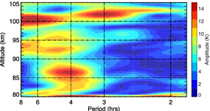
Figure 2. Periodogram as a function of altitude for the neutral
temperature variation derived from the Lomb–Scargle method with oversampling factor 4.
between 80 and 95 km. For example, the higher-temperature (about 230 K) region was seen at about 92 km at 20:00 UT and moved down to about 82 km at 23:00 UT. These temporal and altitude variations of the temperature suggest the signa-ture of a monochromatic gravity wave (GW) propagating up-ward. On the other hand, no periodical temperature variation can be seen above 95 km between 16:30 and 21:00 UT, while a similar (but weaker) temperature variation can be found above 95 km from 21:00 to 24:30 UT. This difference sug-gests that conditions of the background atmosphere changed and affected the propagation of the GW.
Figure 2 shows contours of spectra of the neutral tem-perature from 80 to 100 km for the same time interval as Fig. 1. The Lomb–Scargle periodogram method (cf. Press and Rybicki, 1989; Hocke, 1998) using an oversampling fac-tor of 4 was applied. From Fig. 2, a component with a period of about 4 h is found to be dominant below 90 km, while at 100 km a component of about 8 h is significant. The ampli-tude of the 4 h component reached a maximum at 86 km with a value of∼15 K. It should be pointed out that the 8 h tempo-ral variation found at 100 km is probably not a real periodic component because no clear temporal variation of the tem-perature between 16:30 and 21:00 UT above 95 km is seen in Fig. 1a. When we analyzed temperature data for two time in-tervals separately between 16:30 and 20:30 UT and between 20:30 and 24:30 UT, no salient periodic variation of the tem-perature was found for the earlier interval above 95 km, while a 4 h variation component was found for the latter interval.
1630 1800 1900 2000 2100 2200 2300 2430 UT
80 85 90 95 100 105
Altitude (km)
(b)
1630 1800 1900 2000 2100 2200 2300 2430
UT 80
85 90 95 100 105
Altitude (km)
(b)
-60 -40 -20 0 20 40 60
Northward wind velocity (m/s)
1630 1800 1900 2000 2100 2200 2300 2430
UT 80
85 90 95 100 105
Altitude (km)
(a)
1630 1800 1900 2000 2100 2200 2300 2430
UT 80
85 90 95 100 105
Altitude (km)
(a)
-60 -40 -20 0 20 40 60
Eastward wind velocity (m/s)
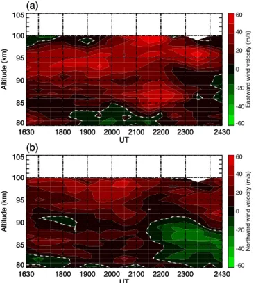
Figure 3.The eastward(a)and northward(b) wind velocity
ob-tained by meteor radar from 80 to 100 km from 16:30 to 24:30 UT on 29 October 2010. White dashed lines indicate zero wind velocity.
speed became lower after 21:00 UT above 90 km, and the wind direction changed from north to south around 21:30 UT below∼90 km.
4 Discussion
We will investigate how the GW disappeared around 95 km before 21:00 UT by evaluating three mechanisms: critical-level filtering and convective and dynamic instabilities. If critical-level filtering prevents a GW from achieving upward propagation, the background wind velocity must be equal to or larger than the horizontal phase velocity of the GW. The square of the Brunt–Väisälä frequency should become nega-tive in the height region if a GW is dissipated by convecnega-tive instabilities. The square of the Brunt–Väisälä frequency,N2, is expressed by
N2= g T
dT dz +Ŵd
, (1)
where g, T, z, and Ŵd are the acceleration of gravity (9.5 m s−2), neutral temperature, altitude, and adiabatic lapse rate in dry air (9.5×10⁻³K m−1). The (bulk) Richardson number is calculated from the following formula:
Ri= N
2
(dduz)2+(dv
dz)2
, (2)
where dduz and ddvz are differential eastward and northward wind velocities, respectively. One of the dynamical instabil-ities in the atmosphere is the Kelvin–Helmholtz (KH) insta-bility, which sets in when the Richardson number (Ri) of the wind profile is less than 0.25 (Drazin, 1958), whereasRi<1 describes conditions still favorable to the instability persist-ing (cf. Szewczyk et al., 2013).
4.1 Critical-level filtering
We have derived horizontal phase velocity, vertical and hor-izontal wave numbers and propagating direction of the GW from the LIDAR temperature data as well as the MR wind data using the hodograph method (Sawyer, 1961). The dis-persion relation, on the assumption that the Boussinesq ap-proximation can be applied for GWs, is shown as
σ=k (c−U )=
f2m2+N2k2
k2+m2
1/2
, (3)
whereσ is intrinsic frequency,kis horizontal wave number, cis the phase velocity of the GW,Uis the background wind speed along with the propagation direction of the GW,f is the inertia frequency (f =1.36×10⁻⁴rad s−1 at Tromsø), andmis the vertical wave number of the GW. The altitude region wherecequalsUis called the critical level, and GW cannot propagate to altitudes above the critical level. This is known as critical-level filtering (cf. Ejiri et al., 2009; Suzuki et al., 2009; Taylor et al., 1993).
The hodograph method is based on the linear theory for GWs (cf. Placke et al., 2013) and has been used to determine the propagation direction as well as phase velocity of GWs (e.g., Yamamoto et al., 1987; Namboothiri et al., 1996). For a monochromatic wave, an ellipse can be drawn. The ma-jor axis of the ellipse indicates the propagation direction, and the direction of rotation as a function of height (from lower height to upper height) indicates the direction of en-ergy transport. The upward propagation of GWs observed in the Northern Hemisphere is subject to a clockwise rotation. Intrinsic frequency of a GW can be obtained from the polar-ization relation
σ=u˜ ˜
vf, (4)
whereu˜ andv˜ are lengths of the major and minor axes, re-spectively.
The dispersion relation can be obtained from Eq. (3) when solved for horizontal wave number (k):
k2= f 2−σ2
σ2−N2m 2.
(5) The vertical wave number (m) can be derived by the hodo-graph method, and N2 can be calculated from the LIDAR temperature data as a function of altitude and time using Eq. (1). Phase velocity is given as follows:
c=ω
-15 -10 -5 0 5 10 15 Eastward Wind (m/s) -15 -10 -5 0 5 10 15
Northward Wind (m/s)
1700UT
-1 deg
80 8182 83
84 85 86 87 88 89 90
91 92 93 94959697
-15 -10 -5 0 5 10 15
Eastward Wind (m/s) -15 -10 -5 0 5 10 15
Northward Wind (m/s)
1800UT -66 deg 80 81 82 83 84 85 86 87 88 89 90 91 92 93 94 95 96 97
-15 -10 -5 0 5 10 15
Eastward Wind (m/s) -15 -10 -5 0 5 10 15
Northward Wind (m/s)
1900UT 12 deg 80 81 82 83 84 85 86 87 88 89
90 91 92
93
94 95 96 97
-15 -10 -5 0 5 10 15
Eastward Wind (m/s) -15 -10 -5 0 5 10 15
Northward Wind (m/s)
2000UT -20 deg 80 81 82 83 84 85 86 87
88 89 90
91 92 93 94 95 96 97
-15 -10 -5 0 5 10 15
Eastward Wind (m/s) -15 -10 -5 0 5 10 15
Northward Wind (m/s)
2100UT 31 deg 80 81 82 83 84 85 86 87 88 89 90 91 92 93 94 95 96 97
-15 -10 -5 0 5 10 15
Eastward Wind (m/s) -15 -10 -5 0 5 10 15
Northward Wind (m/s)
2200UT -16 deg 80 81 88 89 90 91 92 93 94 95 96 97
-15 -10 -5 0 5 10 15 Eastward Wind (m/s) -15 -10 -5 0 5 10 15
Northward Wind (m/s)
2300UT
-13 deg
80 81 8283 84
85 86 87 88 89 90 91 92 93 94 95 96 97
-15 -10 -5 0 5 10 15 Eastward Wind (m/s) -15 -10 -5 0 5 10 15
Northward Wind (m/s)
2400UT 48 deg 80 81 82 83 84 85 86 87 88 89 90 91 92 93 94 95 96 97
-15 -10 -5 0 5 10 15
Eastward Wind (m/s) -15 -10 -5 0 5 10 15
Northward Wind (m/s) 14 deg 14 deg 14 deg 14 deg 14 deg 14 deg 14 deg 14 deg
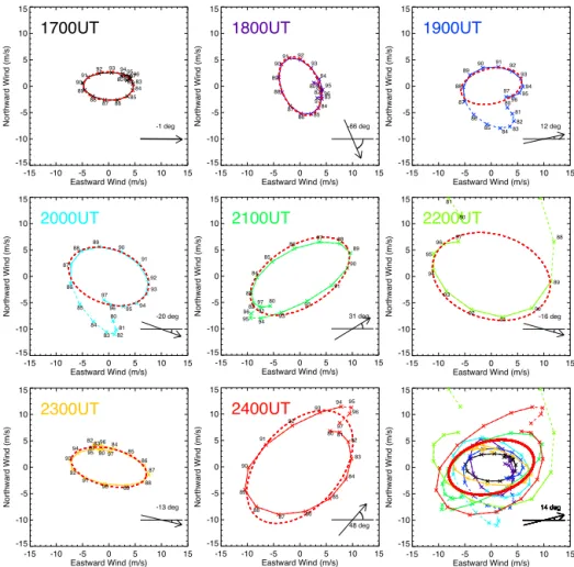
Figure 4.Eight hourly hodographs associated with the fitted eclipses are shown. Crosses denote data values associated with corresponding height values (in km). In the bottom right panel, superimposed hodographs with the fitted ellipse (thicker solid line) are presented. The estimated propagation direction is illustrated in each panel.
where ω is the apparent frequency, and ω=4.36× 10⁻⁴rad s−1 (i.e., 2π/4 h) in this event. By using the hodo-graph method, and Eqs. (4), (5), and (6), we can derive the phase velocity along the propagation direction of the GW.
The hodograph method works properly only for a monochromatic wave event (cf. Lue and Kuo, 2012). It should be pointed out that for the four winter observations of the sodium LIDAR at Tromsø, from October 2010 to March 2014, the current event is one of the most promi-nent monochromatic wave events. In addition, geomagneti-cally, it was a very quiet interval (Kp less than 1); thus, this event is a rare case. For the hodograph analysis, we use MR wind data obtained over 48 h from 00:00 UT on 29 October to 24:00 UT on 30 October 2010. First, the mean wind over pe-riodic components that are 48 h and longer (longer than 8 h) and which are derived by the Lomb–Scargle periodogram method using an oversampling factor of 4 is removed from the wind data. Second, using the 8 h length of wind data from 16:30 to 24:30 UT on 29 October 2010, periodic components are derived by the Lomb–Scargle periodogram method using an oversampling factor of 4, and then shorter components
(shorter than 3 h) are removed from the wind data. Third, a similar procedure is applied for the altitude domain from 80 to 97 km. Then, components utilized for the hodograph anal-ysis that have periods of 3 to 8 h and whose vertical wave-length is longer than 7.5 km are selected from the data sets.
Figure 4 shows eight sets of hourly hodographs (solid lines) from 17:00 to 24:00 UT. Data values (shown by crosses) together with corresponding height values are illus-trated. Furthermore, ellipses (red dashed lines) derived by the least-squares fit and estimated propagation directions are pre-sented in each panel. Some other periodic components seem to be mixed in the hodographs at 19:00, 20:00, and 22:00 UT at lower heights, and we have only used data values at and above 87, 86, and 89 km for the respective times. Given the 180◦ambiguity, we can conclude that the GW propagated to-ward east–northeast/east–southeast or west–southwest/west– northwest.
GW propagation can be divided into two components – east– west and north–south – that are expressed by the apparent frequency (ω), the vertical wave number (m), the phase (φ) of the retrieved wave component, and the propagation direc-tion angle (θ) counted clockwise from east. The following equations are utilized to derive the ellipse:
Ueast= ˜ucos(ωt−mz−φ)cosθ
− ˜vsin(ωt−mz−φ)sinθ, (7)
Unorth= ˜ucos(ωt−mz−φ)sinθ
− ˜vsin(ωt−mz−φ)cosθ. (8)
The major and minor axes of the fitted hodograph (i.e., the ellipse) are 16.5 and 9.95 m s−1, respectively. The propaga-tion direcpropaga-tion is 14◦north (south) from east (west), i.e., al-most eastward or westward. The estimated vertical wave-length is about 11.9 km. By substituting the major and minor axes and the inertial frequency, Eq. (4) gives the intrinsic fre-quency of the gravity wave,σ, as 2.26×10⁻⁴rad s−1, which corresponds to an oscillation period of ∼7.7 h. The square of the Brunt–Väisälä frequency,N2, is 4.41×10⁻⁴rad2s−2 (i.e., the Brunt–Väisälä period being about 5 min) on average (negative values were rejected) between 81 and 95 km from 16:30 to 24:30 UT. Thus, Eq. (5) gives the horizontal wave number (k), i.e., 4.56×10⁻⁶rad m−1, which corresponds to the horizontal wavelength of∼1379 km. Therefore, the hor-izontal phase velocity, c, is calculated to be 96 m s−1 by Eq. (6).
All parameters derived from the hodograph method are listed in Table 1. Since the intrinsic frequency is less than ap-parent frequency, the propagation direction is likely almost eastward. The maximum wind velocity along the estimated propagation direction during the 8 h is 51 m s−1, which is significantly less than c(96 m s−1). Furthermore, as shown in Table 1, the differences (c−U) for the hourly results are always positive. These results indicate that the phase velocity cwas always greater than the background wind velocityU. Therefore, we conclude that critical-level filtering was not a dominant mechanism for the GW disappearing in this event. Another point to be investigated is the similarity of wave-like structures measured with the LIDAR and the MR. Since physical parameters provided with the two instruments dif-fer, to ensure both instruments captured the same GW, we should investigate the relationship below:
˜ θ
=θ ′ ¯ θ
=iN 2
gσ k mu
′
, (9)
whereθ˜is proportion of the fluctuation of the potential tem-perature,θ¯andiare the potential temperature and imaginary unit, andθ′andu′are perturbations of potential temperature and wind velocity along the propagation direction, respec-tively (cf. Fritts and Alexander, 2003). Here, we use the MR wind data obtained for the same interval as the LIDAR tem-perature data from 16:30 to 24:30 UT on 29 October 2010,
16 20 24
Local time of maximum (hr) 80
85 90 95 100
Altitude (km)
Temperature Wind (a)
-2 -1 0 1 2
Difference (hrs) 80
85 90 95 100
Altitude (km)
(b)
80 85 90 95 100
Altitude (km)
0 5 10 15 20
Amplitude (K) 0 5Amplitude (m/s)10 15 20
(c)
Temperature Wind
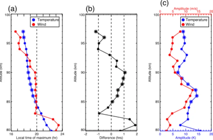
Figure 5.The local time maximum(a), phase difference between
temperature and wind oscillation(b), and amplitude profile of the temperature and wind(c). The red and blue circles denote wind and temperature data, respectively. The period is 4 h. The double circles show values over the 99 % significance level.
andu′=13 m s−1at 87 km (from Fig. 5c). By using the pa-rameter values above, we obtain
˜
θ=∼0.023. (10)
This estimation suggests that perturbation of the background temperature due to the GW should be ∼2.3 %. The av-eraged temperature over the 8 h is ∼216 K at 87 km, and then the temperature perturbation is calculated to be∼5.0 K (=0.023×216), which is about 40 % of the amplitude ob-served by the LIDAR (see Fig. 5c).
According to Eq. (9), the phase of the GW in the temper-ature should precede by 90◦that of the wind along the prop-agation direction (i.e., 1 h for the oscillation period of 4 h). Figure 5a shows height profiles of the phases of the tempera-ture and the wind for the GW (with an apparent period of 4 h) along its propagation direction, and Fig. 5b shows their dif-ferences. Figure 5c shows height profiles of the amplitudes of the temperature (blue) and the wind (red) data. Blue double circles denote the values whose normalized amplitudes are greater than the corresponding 99 % significance levels, and they are located between 85 and 90 km and between 96 and 97 km. The phase difference between 85 and 90 km presented in Fig. 5b shows that phases of the temperature preceded that of the wind by about 0–1 h. When we consider worse tem-poral resolution of the MR (1 h) wind measurements, these results confirm that the LIDAR and the MR have captured the same GW signature.
4.2 Convective and dynamic instabilities
Table 1.Parameters derived with the hodograph method.
Time (UT) u¯(m s−1) v¯(m s−1) θ(rad) c(m s−1) U(m s−1) c−U(m s−1)
17:00 9.51 5.37 −0.02 88.6 38.1 50
18:00 11.6 7.07 −1.17 95.2 39.2 56
19:00 11.6 6.63 0.22 86.2 45.4 40
20:00 15.8 10.3 −0.35 100 50.3 50
21:00 21.0 11.7 0.55 83.6 51.9 32
22:00 22.8 16.0 −0.28 127 47.9 79
23:00 14.6 7.06 −0.23 75.9 51.0 25
24:00 25.0 15.4 0.85 98.5 37.6 61
All 16.5 9.95 0.24 95.8 51.3 45
1630 1800 1900 2000 2100 2200 2300 2430 UT
80 85 90 95 100 105
Altitude (km)
1630 1800 1900 2000 2100 2200 2300 2430 UT
80 85 90 95 100 105
Altitude (km)
0 1 2 3 4 5
N
2 (x10 -4 rad 2/s 2)
Figure 6. Variations of the square of Brunt–Väisälä frequencies
(N2) from 16:30 to 24:30 UT between 81 and 104 km. NegativeN2 regions are shown by blue filled squares.
from 16:30 to 24:30 UT between 81 and 104 km. Negative (N2<0) regions are shown by blue filled squares. The ver-tical temperature gradient, dT /dz, is calculated using neigh-bor data within±1 km height. Below 87 km, there is a ten-dency for the number of negative regions to be larger before 21:00 UT than those after 21:00 UT, while between 87 and 94 kmN2 is almost always positive over the time interval. Between 95 and 100 km, N2is lower before 21:00 UT than after 21:00 UT. Furthermore, there is a tendency for the neg-ative values to occur more frequently before 21:00 UT than after 21:00 UT between 95 and 100 km.
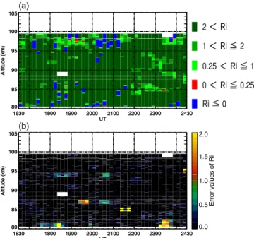
Figure 7a shows variations of the Richardson number from Eq. (2), and Fig. 7b shows their error values. More precisely, thisRishould be called the bulk Richardson number, but, as in many other studies, we call it the Richardson number in this paper. The error values are calculated based on the prop-agation of uncertainties, and they are less than 0.5 for almost the whole time interval. Between 16:30 and 21:30 UT, there is an almost continual layer (about a few km thick) where the Richardson number is less than 2 (including negative values) between 95 and 99 km. The value of 0<Ri<0.25 occurred rarely, but it occurred between 18:50 and 19:40 UT around 97–98 km. Since the almost all-sky horizontal view (∼140◦) as well as poor height (2 km) and temporal (1 h) resolution
1630 1800 1900 2000 2100 2200 2300 2430 UT
80 85 90 95 100 105
Altitude (km)
(b)
1630 1800 1900 2000 2100 2200 2300 2430 UT
80 85 90 95 100 105
Altitude (km)
0.0 0.5 1.0 1.5 2.0
Error values of Ri
1630 1800 1900 2000 2100 2200 2300 2430
UT 80
85 90 95 100 105
Altitude (km)
(a)
1630 1800 1900 2000 2100 2200 2300 2430
UT 80
85 90 95 100 105
Altitude (km)
2 < Ri
1 < Ri ≦ 2
0.25 < Ri ≦ 1
0 < Ri ≦ 0.25
Ri ≦ 0
Figure 7. (a)Variations of the Richardson number from 81 to 99 km between 16:30 and 24:30 UT on 29 October 2010. Negative values are shown by blue filled squares.(b)Error values of the Richardson number.
of the MR induces overestimation ofRi, we are able to say that the shear instability occurred more frequently than the current occurrence of 0<Ri<0.25.
4.3 GW breaking
1630 1800 1900 2000 2100 2200 2300 2430 UT
80 85 90 95 100 105
Virtual Height (km)
180 180
180
180
180 190
190
190
190 190
190
190 190
190
200
200
200 200
200
200
200
200
200
200
200 200
200
200
210
210
210 210
210 210
210
210 210 210
210
210
210
210
220
220
220
220 220
220
230
230
230
1630 1800 1900 2000 2100 2200 2300 2430
UT 80
85 90 95 100 105
Virtual Height (km)
0 20 40 60 80 100
Power (LOG
10
, Arbitrary units)
Figure 8.Variations of MF radar echo intensity from 80 to 105 km (in virtual height) between 16:30 and 24:30 UT on 29 October 2010. The black lines are contours of the neutral temperature (K) shown in Fig. 1a.
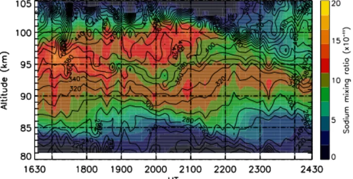
contour lines of the neutral temperature shown in Fig. 1a. Enhancements of the backscatter echo power are found from 18:00 to 21:00 UT above about 90 km, and the echo power decreased sharply after 21:00 UT. This suggests the pres-ence of strong turbulpres-ence above 90–95 km between 18:00 and 21:00 UT. This region corresponds to the region where the Brunt–Väisälä frequency became lower andRiwas lower. Figure 9 shows the sodium mixing ratio as a function of al-titude and time together with potential temperature between 16:30 and 24:30 UT on 29 October 2010. The mixing ratio was calculated in the same way as in the work of Williams et al. (2002), where the measured temperature was utilized to determine the total air density based on hydrostatic relation and ideal gas law (cf. Liu et al., 2004). Potential tempera-ture is defined asT (t, z)(p(t0, z0)/p(t, z))κ, whereT (t, z)is neutral temperature obtained by LIDAR as a function of time (t) and altitude (z),κ is the index of potential temperature (=2/7),p(t, z)is pressure as a function of time and altitude, andt0andz0are the reference time and altitude determined to be 20:30 UT and 81 km, respectively.p(t0, z0)is given by
p(t0, z0)=n(t0, z0)kbT (z¯ 0), (11) wheren(t0, z0)is given by MSIS-E-90 model (Hedin, 1991) and kb is the Boltzmann constant (=1.38×10⁻²³J K−1).
¯
T (z0)(=206 K) is the average value of the observed tem-peratures over the 8 h at 81 km. By assuming the hydrostatic equilibrium, we can calculate the pressure as follows:
p(t, z)=p(t0, z0)exp(−g R
z Z
z0
T (t, h)−1dh), (12)
whereR(=287 J kg−1K−1) is the gas constant (cf. Williams et al., 2002). The atmospheric number density is then calcu-lated from the ideal gas law:
n(t, z)= p(t, z)
kbT (t, z). (13)
Figure 9. The color contours show the sodium mixing ratio
(×10−11) on 29 October 2010. The black lines are contours of the potential temperature (K).
The sodium mixing ratio shows a double peak structure be-tween 18:00 and 21:30 UT. An overturning in the sodium al-titude profile should indicate that a wave is breaking or is about to break (Hecht, 2004). Possible causes of overturning features of the sodium density between 95 and 105 km were discussed by Larsen et al. (2004). Though the causes are still not well understood, an overturning is a common character-istic of Kelvin–Helmholtz instabilities associated with large shears or the manifestation of GW breaking (Larsen et al., 2004).
To summarize the observational results, the region of the lower Richardson number above 95 km corresponds rela-tively well to regions of enhancements of MF radar echo power as well as to the overturning structure of the sodium mixing ratio. Therefore, the dissipation of the GW around 95 km before 21:00 UT would probably be due to wave breaking and the instabilities.
4.4 Possible causes of the difference of the GW propagation
0 5 10 15 20 Amplitude (m/s) 80
85 90 95 100
Altitude (km)
Eastward Northward
8 0 4 8 Local time of maximum (hr) 80
85 90 95 100
Altitude (km)
Figure 10. Altitude profiles of semidiurnal tidal amplitude (left) and local time of maximum (right). Diamonds and triangles denote eastward and northward components, respectively.
tidal amplitudes reached a maximum at 91 km for both the meridional and zonal components with values of ∼16 and ∼13 m s−1, respectively, and minimized at 95–96 km. Since the phase jump is seen around 95 km, it appears that an-other mode grew above 95 km. Around 95 km, the semidi-urnal tidal amplitudes were very small, and thus it seems that the semidiurnal tide did not significantly influence the GW propagation.
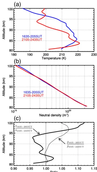
Figure 11 compares background conditions between the two intervals before and after 21:00 UT. In the top panel, altitude profiles of the averaged temperature are compared, and it is found that the shapes of them differ. In particu-lar, between 94 and 100 km, the negative temperature gra-dient (−4.4 K km−1) existed before 21:00 UT, while after 21:00 UT the temperature was relatively constant (associated with small fluctuations) by height. This suggests that the at-mosphere before 21:00 UT tended to become unstable more easily due to wave-induced temperature oscillation than in the later interval. In the middle panel, the neutral densities derived by Eq. (13) are presented for comparison. The aver-aged neutral density before 21:00 UT is larger than that af-ter 21:00 UT above 95 km, while between 85 and 95 km the opposite is true. The difference is presented more clearly in Fig. 11c. In the bottom panel, the ratio of the neutral densi-ties (thick line) as well as the pressure (thin line) derived by Eq. (12) are presented. Between 85 and 95 km the averaged neutral density was larger by up to ∼3 % after 21:00 UT, while between 95 and 100 km it is larger by up to ∼10 % before 21:00 UT. The ratio of the pressure shows that higher pressure occurred above 87 km before 21:00 UT.
To summarize, during the earlier interval (i.e., before 21:00 UT), the neutral density and the pressure were higher – up to ∼10 and∼7 % above 95 and 87 km, respectively – and the steady negative slope of the temperature gradient
180 190 200 210 220 230
Temperature (K) 80
85 90 95 100
Altitude (km)
180 190 200 210 220 230
Temperature (K) 80
85 90 95 100
Altitude (km) 1635-2055UT2105-2435UT
(a)
1019
1020
Neutral density (m-3)
80 85 90 95 100
Altitude (km)
1019
1020
Neutral density (m-3)
80 85 90 95 100
Altitude (km) 1635-2055UT2105-2435UT
(b)
0.90 0.95 1.00 1.05 1.10 1.15
Ratio 80
85 90 95 100
Altitude (km)
0.90 0.95 1.00 1.05 1.10 1.15
Ratio 80
85 90 95 100
Altitude (km)
(c)
¯n1635−2055UT
¯
n2105−2435UT
¯
p1635−2055UT
¯
p2105−2435UT
Figure 11. (a)Altitude profiles of the background temperature are compared for the two intervals between 16:30 and 21:00 UT and 21:00 and 24:30 UT.(b)Same as (a)but for the neutral density. (c)Ratios of neutral density (thick line) and pressure (thin line) be-tween the two intervals.
5 Summary
A monochromatic GW was observed on 29 October 2010 with the sodium LIDAR operated at Ramjordmoen, Tromsø, Norway (69.6◦N, 19.2◦E). The observational data were ob-tained during a geomagnetically very quiet interval (Kp≤1). The spectral as well as the hodograph analyses indicated that apparent period, intrinsic period, vertical and horizon-tal wavelengths, and maximum amplitude were 4 h,∼7.7 h, ∼11.9 km,∼1.38×10³km, and∼15 K, respectively, from 81 to 95 km. The GW dissipated at ∼95 km height from 16:30 to∼21:00 UT, while the GW propagated further over 100 km from 21:00 to 24:30 UT. We evaluated three can-didate mechanisms for the dissipation of the GW: critical-level filtering and the convective and dynamic instabilities. To evaluate critical-level filtering, we compared the back-ground wind velocity and the phase velocity derived by the hodograph method. As a result of the analysis, we have found that the phase velocity is almost always greater than the background wind velocity, indicating that critical-level fil-tering did not play a role in this event. To evaluate the con-vective and dynamic instabilities, we calculated the Brunt– Väisälä frequency (N) and Richardson number (Ri). Before 21:00 UT and between 95 and 100 km, N2is lower and the negativeN2appears to occur more frequently. There was an almost continual layer a few kilometers thick where theRiis smaller (≤2) between 95 and 100 km before 21:20 UT, im-plying that the dynamic instabilities would occur, consider-ing poorer height and horizontal and temporal resolutions of the MR wind data. Because we found enhancements of MF radar power echo before 21:00 UT and an overturning struc-ture of the sodium mixing ratio between 18:30 and 21:30 UT, we concluded that the GW dissipated by wave breaking and the instabilities before∼21:00 UT.
We investigated differences of background atmosphere for the two intervals between 16:30 and 21:00 and 21:00 and 24:30 UT. The most prominent difference is that there was a steady negative slope of the averaged temperature (−4.4 K km−1) between 94 and 100 km before 21:00 UT. We propose that the difference in the temperature profile above 94 km is a probable cause of the change in the GW prop-agation. We need further data sets to investigate this issue in more detail. Since October 2012, the sodium LIDAR at Tromsø has observed wind data together with neutral tem-perature and sodium density data along with five directions (usually, vertical, north, south, east, and west). Thus, we can conduct similar studies in the near future but using wind data with higher height and narrower spatial resolution.
Acknowledgements. The Tromsø sodium lidar project is mainly supported by Special Funds for Education and Research (Energy Transport Processes in Geospace) from the Ministry of Education, Culture, Sports, Science, and Technology in Japan (MEXT), in col-laboration with Nagoya University, Shinshu University, RIKEN, University of Tromsø, and the EISCAT Scientific Association. We
wish to thank M. Ejiri and Y. Tomikawa for their valuable com-ments. We thank K. Hocke for letting us use his Lomb–Scargle peri-odogram method routines. We also acknowledge the use of geomag-netic data from the World Data Centers for Geomagnetism in Kyoto, Japan, and Copenhagen, Denmark, and the Kp indices from Geo-ForschungsZentrum Potsdam (www.gfz-potsdam.de). T. Takahashi is supported as a research fellow of the Japan Society for the Promo-tion of Science (JSPS) for Young Scientists. This research has been partly supported by MEXT through a Grant-in-Aid for JSPS fellows (25-3733), Scientific Research B (22403010, 23340144, 24310010, and 25287126), and Special Funds for Education and Research (En-ergy Transport Processes in Geospace). This research was also par-tially supported by MEXT through the Grant-in-Aid for Nagoya University Global COE Program, Quest for Fundamental Principles in the Universe: From Particles to the Solar System and the Cosmos, and Inter-University Upper atmosphere Global Observation NET-work (IUGONET) . This research was also partly supported by the National Institute of Polar Research through General Collaboration Projects no. 24-10. S. Nozawa thanks the International Space Sci-ence Institute (ISSI) for sponsoring the team (no. 217) meetings.
Topical Editor C. Jacobi thanks F. J. Mulligan and one anony-mous referee for their help in evaluating this paper.
References
Aso, T., Tsuda, T., and Kato, S.: Meteor radar observations at Ky-oto Univ., J. Atmos. Terr. Phys., 41, 517–525, doi:10.1016/0021-9169(79)90075-8, 1979.
Drazin, P. G.: The stability of a shear layer in an unbounded hetero-geneous inviscid fluid, J. Fluid Mech., 4, 214–224, 1958. Ejiri, M. K., Taylor, M. J., Nakamura, T., and Franke, S. J.:
Crit-ical level interaction of a gravity wave with background winds driven by a large-scale wave perturbation, J. Geophys. Res., 114, D18117, doi:10.1029/2008JD011381, 2009.
Fritts, D. C. and Alexander, M. J.: Gravity wave dynamics and effects in the middle atmosphere, Rev. Geophys., 41, 1003, doi:10.1029/2001RG000106, 2003.
Fritts, D. C. and Rastogi, P. K.: Convective and dynamical insta-bilities due to gravity wave motions in the lower and middle at-mosphere: Theory and observations, Radio Sci., 20, 1247–1277, 1985.
Fritts, D. C. and Vadas, S. L.: Gravity wave penetration into the thermosphere: sensitivity to solar cycle variations and mean winds, Ann. Geophys., 26, 3841–3861, doi:10.5194/angeo-26-3841-2008, 2008.
Hall, C. M.: The Ramfjordmoen MF radar (69◦N, 19◦E): applica-tion development 1990–2000, J. Atmos. Sol.-Terr. Phy., 63, 171– 179, 2001.
Hall, C. M., Aso, T., Tsutsumi, M., Nozawa, S., Manson, A. H., and Meek, C. E.: A comparison of mesosphere and lower thermosphere neutral winds as determined by meteor and
medium-frequency radar at 70◦N, Radio Sci., 40, RS4001,
doi:10.1029/2004RS003102, 2005.
Hecht, J. H.: Instability layers and airglow imaging, Rev. Geophys., 42, RG1001, doi:10.1029/2003RG000131, 2004.
imaging, Na lidar, and MF radar observations, J. Geophys. Res., 102, 6655–6668, 1997.
Hecht, J. H., Liu, A. Z., Walterscheid, R. L., and Rudy, R. J.: Maui Mesosphere and Lower Thermosphere e(Maui MALT) observations of the evolution of Kelvin–Helmholtz billows formed near 86 km altitude, J. Geophys. Res., 110, D09S10, doi:10.1029/2003JD003908, 2005.
Hedin, A. E.: Extension of the MSIS thermosphere model into the lower atmosphere, J. Geophys. Res., 96, 1159–1172, 1991. Hocke, K.: Phase estimation with the Lomb-Scargle periodogram
method, Ann. Geophys., 16, 356–358, 1998, http://www.ann-geophys.net/16/356/1998/.
Hodges Jr., R. R.: Generation of turbulence in the upper atmo-sphere by internal gravity waves, J. Geophys. Res., 72, 3455– 3458, 1967.
Holton, J. R.: The role of gravity wave induced drag and diffusion in the momentum budged of the mesosphere, J. Atmos. Sci., 39, 791–799, 1982.
Larsen, M. F., Liu, A. Z., Gardner, C. S., Kelley, M. C., Collins, S., Friedman, J., and Hecht, J. H.: Observations of overturning in the upper mesosphere and lower thermosphere, J. Geophys. Res., 109, D02S04, doi:10.1029/2002JD003067, 2004.
Li, F., Liu, A. Z., Swenson, G. R., Hecht, J. H., and Robinson, W. A.: Observation of gravity wave breakdown into ripples associ-ated with dynamical instabilities, J. Geophys. Res., 110, D09S11, doi:10.1029/2004JD004849, 2005.
Lindzen, R. S.: Turbulence and stress owing to gravity wave and tidal breakdown, J. Geophys. Res., 86, 9707–9714, doi:10.1029/95JD03299, 1981.
Liu, A. Z., Roble, R. G., Hecht, J. H., Larsen, M. F., and Gard-ner, C. S.: Unstable layers in the mesopause region observed with Na liar during the Turbulent Oxygen Mixing Experi-ment (TOMEX) campaign, J. Geophys. Res., 109, D02S02, doi:10.1029/2002JD003056, 2004.
Lu, X., Ziu, A. L., Swenson, G. R., Li, T., Leblac, T., and McDer-mid, I. S.: Gravity wave propagation and dissipation from the stratosphere to the lower thermosphere, J. Geophys. Res., 114, D11101, doi:10.1029/2008JD010112, 2009.
Lue, H. Y. and Kuo, F. S.: Comparative studies of methods of ob-taining AGW’s propagation properties, Ann. Geophys., 30, 557– 570, doi:10.5194/angeo-30-557-2012, 2012.
Meek, C. E.: An efficient method for analysing ionospheric drifts data, J. Atmos. Terr. Phys., 42, 835–839, 1980.
Namboothiri, S. P., Tsuda, T., Tsutsumi, M., Nakamura, T., Na-gasawa, C., and Abo, M.: Simultaneous observations of meso-spheric gravity waves with the MU radar and a sodium lidar, J. Geophys. Res., 101, 4057–4063, 1996.
Nozawa, S., Kawahara, T. D., Saito, N., Hall, C. M., Tsuda, T. T., Kawabata, T., Wada, S., Brekke, A., Takahashi, T., Fujiwara, H., Ogawa, Y., and Fujii, R.: Variations of the neutral temperature and sodium density between 80 and 107 km above Tromsø dur-ing the winter of 2010–2011 by a new solid state sodium LIDAR, J. Geophys. Res., 119, 441–451, doi:10.1002/2013JA019520, 2014.
Placke, M., Hoffmann, P., Gerding, M., Becker, E., and Rapp, M.: Testing liner gravity wave theory with simultaneous wind and temperature data from the mesosphere, J. Atmos. Terr. Phys., 93, 57–69, 2013.
Press, W. H. and Rybicki, G. B.: Fast algorithm for spectral analysis of unevenly sampled data, Astrophys. J., 338, 277–280, 1989. Reid, I. M.: On the measurement of gravity waves, tides and mean
winds in the low and middle latitude mesosphere and thermo-sphere with MF radar, Adv. Space Res., 18, 131–140, 1996. Sawyer, J. S.: Quasi-periodic wind variations with height lower
stratosphere, Q. J. Meteorol. Soc., 87, 24–33, 1961.
She, C. Y. and Yu, J. R.: Doppler-free saturation fluorescence spec-troscopy of Na atoms for atmospheric application, Appl. Optics, 34, 1063–1075, 1995.
She, C. Y., Latifi, H., Yu, J. R., Alverez II, R. J., Bills, R. E., and Gardner, C. S.: Two-frequency LIDAR technique for meso-spheric Na temperature measurements, Geophys. Res. Lett., 31, L24111, doi:10.1029/2004GL021165, 1990.
Suzuki, S., Shiokawa, K., Hosokawa, K., Nakamura, K., and Hocking, W. K.: Statistical characteristics of polar cap meso-spheric gravity waves observed by an all-sky airglow imager at Resolute Bay, Canada, J. Geophys. Res., 114, A01311, doi:10.1029/2008JA013652, 2009.
Szewczyk, A., Strelnikov, B., Rapp, M., Strelnikova, I., Baum-garten, G., Kaifler, N., Dunker, T., and Hoppe, U.-P.: Simulta-neous observations of a Mesospheric Inversion Layer and tur-bulence during the ECOMA-2010 rocket campaign, Ann. Geo-phys., 31, 775–785, doi:10.5194/angeo-31-775-2013, 2013. Taylor, M. J., Ryan, E. H., Tuan, T. F., and Edwards, R.: Evidence of
preferential directions for gravity wave propagation due to wind filtering in the middle atmosphere, J. Geophys. Res., 98, 6047– 6057, 1993.
Thrane, E. V., Blix, T. A., Hall, C., Hansen, T. L., von Zahn, U., Meyer, W., Czechowsky, P., Schmidt, G., Widdel, H.-U., and Neumann, A.: Small scale structure and turbulence in the meso-sphere and lower thermomeso-sphere at high latitude in winter, J. At-mos. Terr. Phys., 46, 119–128, 1987.
Tsutsumi, M., Holdsworth, D., Nakamura, T., and Reid, I.: Meteor observations with an MF radar, Earth Planets Space, 51, 691– 699, 1999.
Vadas, S. L. and Fritts, D. C.: Thermosphere responses to gravity waves arising from mesoscale convective complexes, J. Atmos. Sol.-Terr. Phy., 66, 781–804, 2004.
Williams, B. P., White, M. A., Kruger, D. A., and She, C. Y.: Observation of a large amplitude wave and inversion layer leading to convective instability in the mesopause region over Fort Collins, CO (41N, 105W), Geophys. Res. Lett., 29, 1850, doi:10.1029/2001GL014514, 2002.
Yamamoto, M., Tsuda, T., Kato, S., Sato, T., and Fukao, S.: A Saturated inertia gravity wave in the Mesosphere Observed by the Middle and Upper atmosphere radar, J. Geophys. Res., 92, 11993–11999, 1987.