ABSTRACT: The present work is primarily concerned with studying the effects of artiicial dissipation and of certain diffusive terms in the turbulence model formulation on the capability of representing turbulent boundary layer lows. The lows of interest in the present case are assumed to be adequately represented by the compressible Reynolds-averaged Navier-Stokes equations, and the Spalart-Allmaras eddy viscosity model is used for turbulence closure. The equations are discretized in the context of a general purpose, density-based, unstructured grid inite volume method. Spatial discretization is based on the Steger-Warming lux vector splitting scheme and temporal discretization uses a backward Euler point-implicit integration. The work discusses in detail the theoretical and numerical formulations of the selected model. The computational studies consider the turbulent low over a lat plate at 0.3 freestream Mach number. The paper demonstrates that the excessive artiicial dissipation automatically generated by the original spatial discretization scheme can deteriorate boundary layer predictions. Moreover, the results also show that the inclusion of Spalart-Allmaras model cross-diffusion terms is primarily important in the viscous sublayer region of the boundary layer. Finally, the paper also demonstrates how the spatial discretization scheme can be selectively modiied to correctly control the artiicial dissipation such that the low simulation tool remains robust for high-speed applications at the same time that it can accurately compute turbulent boundary layers.
KEYWORDS: Computational luid dynamics, Turbulence modeling, Flux vector splitting scheme, Artiicial dissipation.
A Study of Physical and Numerical Effects
of Dissipation on Turbulent Flow Simulations
Carlos Junqueira-Junior1, Joao Luiz F. Azevedo2, Leonardo C. Scalabrin3, Edson Basso2INTRODUCTION
he present work is primarily interested in studying the efects of artiicial dissipation and of certain difusive terms in the turbulence model formulation on the capability of representing turbulent boundary layer lows. his interest comes from the fact that situations could arise in which one has a certain computational luid dynamics (CFD) tool, for instance, developed elsewhere, and wants to apply this code to a particular application. It is clear that all decisions taken in the selection of the computational tool, from the choice of a speciic turbulence model to numerical issues, such as the type of spatial discretization used, may have consequences on the quality of numerical results that might be obtained from the simulations. he research group, in the context of which the present efort is inserted, has recently experienced exactly this sort of situation. herefore, an extensive study on the efects of artiicial dissipation had to be performed in order to be able to correctly reproduce turbulent boundary layer lows. Similar issues with the efect of artiicial dissipation terms on boundary layer lows have been previously addressed in the literature (Bigarella, 2007; Bigarella and Azevedo, 2012). However, this previous work is mostly concerned with centrally-diferenced schemes and explicitly added artiicial dissipation, whereas the present efort focuses on the artiicial dissipation terms that arise from an upwind, lux-vector splitting-type discretization. Furthermore, the present study also addressed the decision to include, or not, some terms of the turbulence model formulation in the implemented code, since some of them, in many turbulence models, are computationally stif and, hence, expensive. hus,
1.Instituto Tecnológico de Aeronáutica – São José dos Campos/SP – Brazil 2.Instituto de Aeronáutica e Espaço – São José dos Campos/SP – Brazil
3.EMBRAER – São José dos Campos/SP – Brazil
Author for correspondence: Carlos Junqueira-Junior | Praça Marechal Eduardo Gomes, 50 – Vila das Acácias | CEP 12.228-900 São José dos Campos/SP – Brazil |
E-mail:[email protected]
many investigators simply do not include these troublesome terms in their implementation of such particular model.
he present research group has been focusing on diferent aspects of CFD in the past years. For instance, the group maintains lines of work (Bigarella, 2007; Bigarella et al., 2007; Bigarella and Azevedo, 2009) aimed at creating new capabilities on numerical methods, multigrid techniques, and turbulence modeling. he study of such aspects is also a major issue in the present work. Previous efort was primarily geared towards the simulation of satellite launch vehicle (SLV) lows, which is one of the main interests of Instituto de Aeronáutica e Espaço. It resulted in a powerful Navier-Stokes solver, known as BRU3D, frequently used by the research group.
Additional effort at the group has also addressed the issue of high-order methods (Wolf, 2006; Wolf and Azevedo, 2006 and 2007; Breviglieri, 2010; Breviglieri et al., 2010a and b), and successful applications of schemes such as essentially nonoscillatory (ENO) and weighted essentially nonoscillatory methods (WENO), and spectral methods have been demonstrated. Basso (1997) used preconditioning matrices to extend CFD codes for all speed applications. All these numerical technologies are applied on aeronautical and aerospace simulations, such as high lift and drag predictions, aerodynamics optimization, aeroacoustics, turbulent flows, and wind tunnel validation. The version of the BRU3D code of interest herein is a serial Navier-Stokes solver developed to simulate three-dimensional (3-D) viscous turbulent flows over general aerospace configurations. he code presents diferent turbulent closures such as linear eddy-viscosity turbulence models, explicit algebraic Reynolds-stress models – EARSM (Wallin and Johansson, 2000; Hellsten and Laine, 2000), and Reynolds-stress models – RSM (Batten et al., 1999). A thorough study of flux computational schemes was also undertaken during the development of the code. Spatial discretization of the BRU3D code can be performed with the second-order accurate centered scheme of Jameson et al. (1981) and the Roe flux-difference splitting upwind scheme (Roe, 1981). Different artificial dissipation terms are also added for the Jameson centered spatial discretization (Jameson et al., 1981), such as the convective upwind split pressure (CUSP) scheme (Jameson, 1995a and b), scalar and matrix versions of switched second-difference and fourth-second-difference models (Mavriplis, 1988; Turkel and Vatsa, 1990). The efforts of Bigarella
(Bigarella, 2007; Bigarella and Azevedo, 2009) provided extensive expertise on turbulence modeling, which is a pacing item in CFD (Chapman, 1981).
On the other hand, previous work by Scalabrin and collaborators (Scalabrin, 2007; Scalabrin and Boyd, 2007; Schwartzentruber et al., 2007; Schwartzentruber et al., 2008) developed a numerical tool using upwind schemes, unstructured meshes, high-performance computing (HPC), and implicit integration for numerical simulations of weakly ionized hypersonic lows over reentry capsules. Such research has resulted in a very eicient numerical framework, called LeMANS, to simulate reentry lows over space capsules. hese extreme conditions demanded the implementation of the Navier-Stokes equations coupled to nonequilibrium chemical reaction equations. he computation of these sets of equations requires very ine meshes, which makes impractical the use of serial algorithms. herefore, message passing interface (MPI) protocols were implemented to parallelize LeMANS and, then, reduce computational costs. One should understand that high-idelity CFD solvers have very complex algorithms and, hence, their parallelization involves advanced numerical and computational issues. hus, a full parallel code, as LeMANS, is always welcome. Furthermore, since LeMANS already incorporates several programming issues and high-speed low physics models, it seems to be a more suitable code for continued developments in the future.
In this context, an important motivation of the present work is to take full advantage of all scientiic technology concerning turbulence modeling, boundary condition, and initial condition treatment implemented in the BRU3D solver in order to extend the LeMANS code for the research group needs, more speciically, parallel turbulent low simulations for high dissipative spatial discretization, which are strongly recommended for high-speed conigurations, such as reentry lows. However, such highly dissipative methods can strongly deteriorate boundary layer low predictions. It is clear that the challenge is to selectively modify the discretization scheme in order to correctly control the artiicial dissipation such that the low simulation tool remains robust for high-speed applications, at the same time that it can accurately compute turbulent boundary layers.
artiicial dissipation of the upwind spatial discretization scheme, and the inclusion of numerically stif cross-difusion-like terms in the formulation of the turbulence model. For the present study, the Spalart-Allmaras turbulence model was selected, primarily because it is probably the most widely used turbulence closure for realistic aerospace applications at the time the study was carried out.
his study considers the case of freestream Mach number equal to 0.3, because there are experimental and other independent computational results available. Moreover, since all computational codes here considered implement a compressible formulation, there are no issues with the incompressible limit at such Mach number. he paper demonstrates that the excessive artiicial dissipation automatically generated by the original spatial discretization scheme can deteriorate boundary layer predictions. he paper also demonstrates how the spatial discretization scheme should be selectively modiied to correctly control the artiicial dissipation. Finally, the results show that the inclusion of Spalart-Allmaras model cross-difusion terms is primarily important in the viscous sublayer region of the boundary layer.
THEORETICAL FORMULATION
he formulation used in the present work is based on the Reynolds-averaged Navier-Stokes set of equations, also known by the CFD community as RANS equations. hey are obtained by iltering the Navier-Stokes set of equations. his process ilters the luctuation part of the luid and maintains only the mean contribution. he iltered information needs to be recovered somehow. Turbulence models are applied to the RANS formulation to recover the efect of the luctuating part. he levels of turbulence modeling are also discussed in this section. he most used iltering processes are based on the time, space, and ensemble averages. he iltering based on the time average is the most used for steady state applications and it is the one applied in the present work. For the sake of simplicity, the iltering process is not discussed in this work. he reader can ind further details on the work of Bigarella (2007) and Junqueira-Junior (2012).
he iltered compressible Reynolds-averaged Navier-Stokes equations are written in the vector form as
∂Q
∂t +∇·(F e−F v)=0 . (1)
he conserved variables vector, Q, the inviscid lux vector, Fe, and viscous lux vector, Fv, are given by
v
ρ
Q = ρ ρu ρv ρw e
, F e=
v
ρu + pˆix ρvv + pˆiy
ρwv+ pˆiz
(e + p)v
, Fv= 0 τxi +τxit ˆii τyi +τyit ˆii τzi +τzit ˆii βi +βit ˆii
,
┌ │ │ │ │
└ ┌
│ │ │ │ └
┌ │ │ │ │
└ ┌
│ │ │ │
└ ┌
│ │ │ │
└ ┌
│ │ │ │ └ (
( (
(
) ) )
)
(2)
where ρ stands for the density, v = {u, v, w} is the velocity vector in Cartesian coordinates, p is the static pressure, τ is the viscous stress tensor, qH is the heat lux vector, e is the total energy per unit volume, and βi is given by
βi =τij ˜uj −qHi . (3)
he îx, îy, and îz terms are the Cartesian coordinate orthonormal vector basis. he { } ̅ terms are the averaged and weighted averaged properties. herefore, it is very important to emphasize that ield forces, such as gravity, are neglected here.
Other equations are necessary in order to close the system of equations given by Eq. (2), which are called constitutive relations. The first constitutive equation presented to close the Navier-Stokes set is known as the equation of state. This equation considers the perfect gas law, and it is written as
p =(γ −1) e−1 2 ρ u
2
+ v2+ w2 ,
┌ │
└ ┌
│ └
( ) (4)
in which the mean total energy per unit volume, e ̅, is given by
e =ρ ei+ 1
2 u
2+ v2+ w2 , ┌
│
└ ┌
│ └
( ) (5)
and istands for the internal energy, deined as
ei = CvT , (6)
in which T stands for the mean static temperature and Cv is the speciic heat at constant volume. he heat lux from Eq. (2) is obtained from the Fourier law for heat conduction, and it is given by
qH j=− γµ P
∂(ei)
∂xj ,
in which γ is the ratio of speciic heats and Pr is the Prandtl number. Typically, for air, it is assumed that γ = 1.4 and Pr = 0.72. Cp is the gas speciic heat at constant pressure, and µ is the dynamic molecular viscosity coeicient, calculated as a function of the temperature by the Sutherland law equation (Anderson, 1991), written as
µ = µ∞ T
T∞ 2 3 T∞+ S
T + S ,
⎛ ⎥
⎝ ⎛
⎥ ⎝
(8)
In the above equation, S = 110K, and µ∞ is the dynamic molecular viscosity coeicient of the luid at temperature T∞. he components of the viscous stress tensor, for a Newtonian luid, are given by
τij= µ ∂ui ∂xj +
∂uj ∂xi −
2 3
∂um ∂xm δij
,
┌ │
└ ┌
│ └ ⎛
⎥
⎝ ⎛
⎥ ⎝
(9)
in which δij stands for the Kronecker delta.
All the terms marked with the superscript { }t, in Eq. (2), appear ater the time iltering processes. hese terms carry important turbulent information and need to be modeled. he turbulence closures are responsible for representing them. here are two major families of turbulence models for the RANS equations, the irst and second order closures. he present paper focuses on the irst order closures, more speciically, on the Spalart and Allmaras (1992) model, which is an one-equation closure. his model was chosen because it is, by far, the most used turbulence model for realistic aerospace applications. Furthermore, the research group has already achieved good results using it on previous applications (Bigarella, 2007; Bigarella et al., 2007; Bigarella and Azevedo, 2009). he Spalart-Allmaras turbulence closure is a partial diferential equation, which models the turbulent eddy viscosity transport. he theoretical and numerical formulations of the turbulence closure are discussed in details in the forthcoming sections.
NUMERICAL FORMULATION
SPATIAL DISCRETIZATION
he spatial discretization used is the irst aspect to be discussed in this section, starting with the inite volume formulation and followed by the lux calculations. For the
sake of simplicity, from here, all the averaged terms are written without the { } ̅ notation.
Finite volume formulation
he inite volume formulation is a numerical method applied to represent and evaluate partial diferential equations. It is applied by the CFD community to ind the solution of the RANS equations, Eq. (1). he method is obtained integrating the low equations for each control volume within a given mesh,
Vi
∂Q
∂t dV + Vi∇·(F e−F v)dV=0 . ⌠
⌡ ⌡⌠ (10)
Considering a cell-centered formulation, Vi is a determined cell of the given grid. Ater the integration, it is possible to apply the Gauss theorem over Eq. 10, resulting in
Vi
∂Q
∂t dV + Si (F e−F v) · dS = 0 ,
⌠
⌡ ⌡⌠ (11)
in which Si is the outward-oriented area vector and it is deined as
Si= {Sx , Sy , Sz} . (12) Considering the mean value of the conserved variables within the i-th control volume, one can write the irst term of Eq. (11) as
Qi = 1
Vi Vi
QdVi .
⌠
⌡ (13)
he second term of Eq. (11) can be written as the sum of all faces of a cell
Si
(F e−F v)· dS =
nf
∑
k =1 →
F ek − →F vk · nk→Sk ,
( )
⌠
⌡ (14)
in which the k subscript is the index of the cell face, and nf indicates the number of faces of the i-th volume. Finally, the RANS equations discretized with a inite volume approximation is given by
∑
∂Qi
∂t = −
1
Vi nf
k =1
F ek−F vk · nk Sk .
( → → ) → (15)
Inviscid lux calculation
he inviscid luxes are calculated using a method based on a classical lux vector splitting formulation, the Steger-Warming scheme (Steger and Warming, 1981). he formulation implemented to compute the inviscid luxes is explained here. his method is an upwind scheme that uses the homogeneous property of the inviscid lux vectors to write
F ek· nk = F en =
∂F en
∂Q Q = AQ ,
→ →
(16)
where Fenis the normal lux at the k-th face, and A is the Jacobian matrix of the inviscid lux that can be diagonalized by the matrices of its eigenvectors from the let and from the right, L and R, respectively, as
A = RΛL , (17)
and Λ is the diagonal matrix of the eigenvalues of the Jacobian matrix. he A matrix can be split into positive and negative parts as
A+ = RΛ+ L and A−= RΛ−L . (18)
he splitting separates the lux into two parts, the downstream and the upstream luxes, in relation to the face orientation as
F e · n = F e+n + F e−n = A+( clQcl + Acr−Qcr) ,
→ → (19)
where the cl and cr subscripts are the cells on the let and right sides of the face. he split eigenvalues of the Jacobian matrix are given by
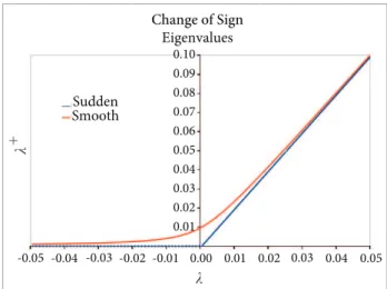
λ± = 1
2(λ± |λ|) . (20)
In order to avoid sudden sign transitions, as illustrated in Fig. 1, the split eigenvalues receive a small number, ϵ, turning Eq. (20) into
λ± = 1 2 λ± λ
2+ϵ2 .
( )√ (21)
Numerical studies performed in the present paper indicated that this lux vector splitting is too dissipative and it can deteriorate the boundary layer proiles (MacCormack and Candler, 1989; Junqueira-Junior et al., 2011). To avoid such
issue a pressure switch is implemented to smoothly shit the Steger-Warming scheme into a centered one. hen, the artiicial dissipation is controlled and the numerical stability is maintained as presented in
→ →
F ek· nk= F +k + F
−
k = A+k+ Qk++ A
−
k− Qk− ,
( ) (22)
in which
Qk+= (1−w)Qcl+wQcr and Qk−= (1−w)Qcr+wQcl . (23)
he switch, w, is given by
w = 1
2 1
(α∇p)2+1 and ∇p =
|pcl −pcr|
min(pcl, pcr)
. (24)
herefore, for small ∇p, w = (1–w) = 0.5, the code runs with a centered scheme, and for larger values of ∇p, w = 0 and (1–w) = 1, the code runs with the Steger-Warming scheme. For Eq. (24), it is suggested α = 6, but some problems may require larger values (Scalabrin, 2007).
he applied formulation was originally created with interest on studying lows over reentry capsules. For this particular case, with very strong shock waves, it is very common to ind solutions with nonphysical numerical structures such as carbuncles (Ramalho et al., 2011). To prevent such numerical problems, artiicial dissipation has necessarily to be added to the method. he dissipation was included into the split eigenvalues, Eq. (21), using the ϵ factor, which is given by:
λ
λ
+
Change of Sign Eigenvalues
Sudden Smooth
0.10 0.09 0.08 0.07 0.06 0.05 0.04 0.03 0.02 0.01
-0.05 -0.04 -0.03 -0.02 -0.01 0.00 0.01 0.02 0.03 0.04 0.05
k=
0.3(ak + |→uk|) dk > d0 0.3(1−|→nk ·→mk|)(ak + |→uk|) dk < d0
, ϵ ⎨⎧
⎩ (25)
where dk is the distance of the k-th face to the the nearest wall boundary, d0 is set by the user and must be smaller than the boundary layer thickness and larger than the shock stand-of distance, mk→ is the normal vector of the nearest wall, and nk→ is the normal vector to the k-th face. Equation (25) applies the term (1 - |nk→ ·mk→|) to decrease the ϵ value at the faces parallel to the wall inside the boundary layer (Scalabrin, 2007). his artiicial dissipation model has shown an important role in the prediction of boundary layer proiles, and several tests were performed in the present work with the aim of understanding its behavior (Junqueira-Junior et al., 2011).
Viscous lux calculation
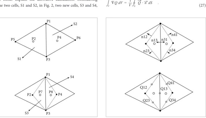
he viscous terms are based on derivative of properties on the faces. To build the derivative terms, two volumes are created over the face where the derivative is being calculated. At the center of each new volume, the derivative is calculated using the Green-Gauss theorem. his computation is used to ind the derivative at the desired face.
A two-dimensional (2-D) example is used in this section to better explain the derivative calculation. Considering the two cells, S1 and S2, in Fig. 2, two new cells, S3 and S4,
are created using node points, P1 and P3, and cell centered points, P2 and P4, to calculate the derivative on the face 1-3.
he properties at the faces are calculated using simple averages. For the example in Fig. 2, they are given by
Q12=1
2(Q1+ Q2) ,
Q23=1
2(Q2+ Q3) ,
Q13= Q31 = 1
2(Q1+ Q3) ,
Q34=1
2(Q3+ Q4) ,
Q41=1
2(Q4+ Q1) .
(26)
Using the averaged properties, Q12, Q23, Q13, Q34, and Q41, with the normal vectors, n12, n23, n13, n34, and n41, and the surface of the faces, S12, S23, S13, S34, and S41, as illustrated in Fig. 3, it is possible to calculate the derivative at the points P7 and P8 using the Green-Gauss theorem (Jawahar and Kamath, 2000), which is applied to a scalar and relates the volume integral of the gradient of its area integral over the boundary as
V
∇Q dV = 1
V S
→
Q ·→n dS .
⌠
⌡ ⌡⌠○ (27)
P 1
P 2
P 3
P 3 P 1
P 4 P 6
S2
P 5
S1
P 7 P 8
P 2 P 4
S3
S4
Figure 2. 2-D example of a new volume creation.
n12 n13
Q 12
Q 23
Q 13 Q 41
Q 34 n31
n41
n34 n23
Considering ∇Q as a constant over the cell, Eq. 27 yields
∇Q = 1 V
→
Q ·→n dS , S
⌠
⌡○ (28)
in which ∇Q is the constant cell-centered gradient. Using the derivatives in the cells S3 and S4, the derivative at face 1-3 is computed using
∇Q13 = ∇ ∇ V3 Q3+ V4 Q4
V3+ V4 . (29)
he derivative computation for other types of element, 2D or 3D, is straightforward.
TIME INTEGRATION
Simulations of turbulent lows can become very stif. Such stifness substantially limits the use of large time steps. One classical solution is the use of implicit time integration. his work applies an implicit integration based on the backward Euler method, which is given by
∆Qncl
∆t Vcl= −
nf
k =1
→
F ek − →F vk ·→nkSk n +1
= Rn +cl 1 .
⎡
⎣ ∑ ( ) ⎤⎦ (30)
One can linearize the residue at time n+1 as a function of properties at time n.
∆Qncl
∆t Vcl= R
n
cl−
nf
k =1
∂ →F e ·→n ∂Q
n
k
∆Qcln −
∂ →F v ·→n ∂Q
n
k∆
Qncl · Sk . ∑ ⎧⎨ ⎩ ⎫ ⎬ ⎭ ⎡ ⎜ ⎣ ⎜ ⎤ ⎦ ⎡ ⎜ ⎣ ⎜ ⎤ ⎦ ( )
( ) (31)
From the spatial discretization, the inviscid terms can be written as
∂ →F e ·→n
∂Q k∆Qcl=
∂ F e→+·→n
∂Q k∆Qcl+
∂ →F e−·→n ∂Q
k
∆Qcl ,
⎡ ⎜ ⎣ ⎜ ⎤ ⎦ ⎡ ⎜ ⎣ ⎜ ⎤ ⎦ ⎡ ⎜ ⎣ ⎜ ⎤ ⎦ ( ) ( )
( ) (32)
with
∂ F e→+ ·→n
∂Q k ∆Qcl = A + k+∆Qcl
⎡ ⎜ ⎣ ⎜ ⎤ ⎦ ( ) (33) and → ∂ F e−·→n
∂Q
k
∆Qcl = A−k− ∆Qcr .
⎡ ⎜ ⎣ ⎜ ⎤ ⎦ ( ) (34)
he formulation described assumes
→ ∂ F e±·→n
∂Q = A
± , ⎡ ⎜ ⎣ ⎜ ⎤ ⎦ ( ) (35)
which is not true and can decrease the numerical stability of the method. hen, the true Jacobian matrices of the split luxes were implemented in place of A± to calculate the implicit operator. Issues involving the true Jacobians matrices have a great importance in the context of numerical stability for computational methods. he reader with interest in this subject must look further in references Anderson et al. (1986) and Steger and Warming (1981), and in chapter 20 from Hirsch (1990).
he viscous terms can be written in the same form as
∂ →F v ·→n
∂Q k
∆Qcl = ∂ →F v −
·→n
∂Q k
∆Qcl−
∂ →F v+·→n
∂Q k
∆Qcl . ⎡ ⎜ ⎣ ⎜ ⎤ ⎦ ⎡ ⎜ ⎣ ⎜ ⎤ ⎦ ⎡ ⎜ ⎣ ⎜ ⎤ ⎦ ( ) ( ) ( ) (36)
he viscous Jacobian matrices are represented by B. he splitting of these matrices is written as
∂ F v ·→ →n
∂Q k∆Qcl =B−k−∆Qcr,k−B +
k+∆Qcl .
⎡ ⎜
⎣ ⎜
⎤
⎦
( ) (37)
he true Jacobian matrices, for A± and B±, can be found in the work of Scalabrin (2007). One can write the system as
Vcl ∆t +
nf
k =1
A+k+ + B
+
k+ Sk ∆Q +
nf
k =1
A−k−−Bk−−Sk∆Qcr,kn = Rn
cl n cl . ∑ ∑ ⎡ ⎜ ⎣ ⎜ ⎤ ⎦ ⎡ ⎜ ⎣ ⎜ ⎤ ⎦ ( ) (38)
It is, then, possible to write
Mcl∆Qncl + nf
k =1
Nk−∆Qncr,k=Rncl ,
∑ (39)
with
Mcl= Vcl ∆t
nf
k =1N
+
k ,
Nk+= A( )+k++ Bk++ Sk (41) and
Nk−= A−k−−B
−
k− Sk .
( ) (42)
As the code is an unstructured solver, this system of equations results in a sparse block matrix, where each block is a square matrix of size equal to the number of equations to be solved in each control volume. he solution of such system is typically very expensive and, depending on the size of the mesh, it is not even practical. A less expensive implicit method is applied in the present paper, the point implicit integration (Gnofo, 2003; Venkatakrishnan, 1995; Wright, 1997).
he main idea of the point implicit integration is to move all the of-diagonal terms to the right hand side and solve the resulting system iteratively, i.e.,
Mcl∆Qn +cl 1,p= R n cl−
nf
k =1 Nk−∆Q
n +1,p−1
cr,k .
∑ (43)
It is assumed that ∆Qn+1,0 = 0 and four iterations are taken in the process as suggested in the literature (Wright, 1997). The sparse linear system illustrates the point implicit method:
∆Q(n +1)
= Rn ,
∆Q(n +1),p = Rn−
∆Q(n +1) ,p −1 . ⎡ ⎜ ⎜ ⎜ ⎜ ⎣ ⎜ ⎜ ⎜⎜ ⎤ ⎦ ⎡ ⎜ ⎜ ⎜ ⎜ ⎣ ⎜ ⎜ ⎜⎜ ⎤ ⎦ ⎡ ⎜ ⎜ ⎜ ⎜ ⎣ ⎡ ⎜ ⎜ ⎜ ⎜ ⎣ ⎜ ⎜ ⎜⎜ ⎤ ⎦ ⎡ ⎜ ⎜ ⎜ ⎜ ⎣ ⎡ ⎜ ⎜ ⎜ ⎜ ⎣ ⎡ ⎜ ⎜ ⎜ ⎜ ⎣ ⎡ ⎜ ⎜ ⎜ ⎜ ⎣ ⎜ ⎜ ⎜⎜ ⎤ ⎦ ⎜ ⎜ ⎜⎜ ⎤ ⎦ ⎜ ⎜ ⎜⎜ ⎤ ⎦ ⎜ ⎜ ⎜⎜ ⎤ ⎦ ⎜ ⎜ ⎜⎜ ⎤ ⎦
Each , in the sparse matrix, is a block matrix. he time step is computed by
∆t = CF L
||→v || + a , (44)
in which CFL (Azevedo, 1988) is a parameter set to ensure stability of the time integration method, l is the size of the cell and || -v || + a is the largest wave speed in the cell (Scalabrin, 2007).
SECOND-ORDER EXTENSION OF INVISCID FLUXES he monotone upstream-centered scheme for conservation laws, known as MUSCL approach (van Leer, 1979), is used
in order to obtain second-order extension for the inviscid luxes calculation. his section presents the classical formulation of the MUSCL approach and an extension for unstructured grids.
MUSCL approach
A irst-order spatial discretization is equivalent to represent the numerical approximation of the solution as a piecewise constant. he MUSCL idea is to use a linear approximation to achieve a second-order space discretization. A linear solution is exactly resolved, which generates a truncation error of the order ∆x2. In order to represent the conservation laws, the discrete state variables express the average state within the cells. hen, the linear approximation has to average out these values (Hirsch, 1990).
One can consider the Taylor linearization as a one-dimensional (1-D) local representation, Fig. 4, valid in a given cell “i”, at a determined instant
Q(x) = Qi+ 1
∆x(x−xi)δiQ +O ∆x
2 x
i−1/2<x<xi +1/2 . ( ) ( ) (45)
setting x = xi ± ∆x/2, it is possible to write
QLi +1/2= Qi+ 1
∆x xi+
∆x
2 −xi δiQ = Qi+12δiQ ,
( ) (46)
QRi−1/2= Qi+ 1
∆x xi−
∆x
2 −xi δiQ = Qi−12δiQ .
( ) (47)
he use of backward and forward derivatives provides
Qi + L 1/2= Qi+21( Qi−Qi−1) , (48)
QRi−1/2= Qi−1
2( Qi +1−Qi) . (49)
One can rewrite these terms at the same faces as
QLi + 1/2(x) = Qi +1
2(Q i−Qi−1) , (50)
QRi + 1/2(x) = Qi +1− 1
2( Qi +2−Qi +1) . (51)
Using limiters to treat correctly the discontinuities, the MUSCL scheme can be written as
QLi + 1/2(x) = Qi+ 1
2ψ r
L Q
i−Qi−1 ,
( )( ) (52)
QRi + 1/2(x) = Qi +1−1
2ψ r
L
Qi +2−Qi +1 ,
where r is the ratio of consecutive variations, given by
rL=Qi +1 −Qi Qi −Qi−1
, rR= Qi +1 −Qi Qi +2 −Qi +1
, (54)
and ψ(r) is a limiter function. h ese functions are extremely important in the context of high-order methods. However, this discussion is not in the scope of the present work. One can i nd further information about limiter functions in chapter 21 from Hirsch (1990).
h ere are several limiter functions available for high-order methods of CFD applications. Two of these functions are implemented herein, the van Albada limiter (van Albada et al., 1982), given by
ψ(r)=r 2
+r
1+r2 , (55)
and the minmod limiter (Hirsch, 1990), written as
ψ(r)= min[r,1],r>0
0 ,r≤0 .
⎧ ⎨
⎩ (56)
h e simulations performed in the present work used mainly the van Albada limiter function (Hirsch, 1990).
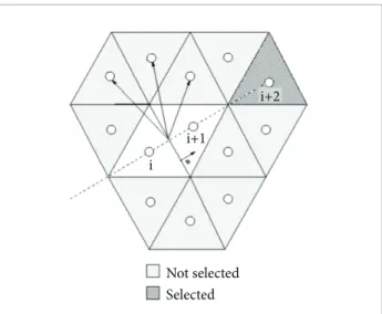
Second-order extension for unstructured grids h e MUSCL variable extrapolation for 2-D or 3-D is straightforward for structured meshes. However, it is not very simple for unstructured solvers. h e approach applied here is based on the work of Batina (1990) and Bibb et al. (1997). Here, the stencils are created using only cell-centered values. h e points “i” and “i+1” are, respectively, the center of the cell at the let and right of the face. h e other two points, “i-1” and “i+2”, are dei ned by a stencil search.
h e search for cells “i+2” and “i-1” is limited to the ones that share at least one node with the volumes “i+1” and “i”, respectively. h e selected “i+2” point is the one that has the maximum positive value of the dot product between the face normal and the normalized vector joining the face centroid
to cell centroid. Using the same principle, the chosen “i-1” point is the one with the maximum negative value of the dot product. Figure 5 is extracted from Scalabrin (2007), and illustrates the search for the “i+2” point in a given mesh.
It is possible to observe that, when the stencil search is applied to unstructured grids, the distance between the “i+1” and “i+2” points can be dif erent from the distance between the “i” and “i+1” points. h erefore, a correction is applied on the limiter, as given by
rL
=Qi +1 −Qi Qi−Qi−1 b
a , r
R
= Qi +1 −Qi Qi +2 −Qi +1
c
a , (57)
where “a” is the distance between the “i+1” and “i” points, “b” is the distance between the “i+2” and “i+1”points, and “c” is the distance between the “i” and “i-1” points.
TURBULENCE MODELING
THE SPALART-ALLMARAS TURBULENCE MODEL h e Spalart-Allmaras (SA) closure (Spalart and Allmaras, 1992 and 1994) is a one-equation, linear eddy-viscosity turbulence model. It solves one transport equation for the modii ed eddy viscosity coei cient, ~ν. h e model uses eight closure coei cients and three closure functions derived along intuitive and empirical lines, relying heavily on calibration by reference to a wide range of experimental data (Spalart Figure 5. Search for the “i + 2” point inside an unstructured grid. (Scalabrin, 2007).
Not selected Selected
i+1
i
i+2
i-1 i
i+1/2
i+1 i-1/2
and Allmaras, 1992 and 1994). he one equation model is originally written as
∂˜ν ∂t+∂
(˜νuj)
∂xj
= cb1S ˜˜ν−cw1fw
˜ ν d 2 + 1 σSA ∂ ∂xj (ν
+ ˜ν) ∂ν˜
∂xj
+cb2 σSA
∂˜ν ∂xk
∂ν˜ ∂xk . ⎛ ⎝ ⎞⎠ ⎡ ⎣ ⎤⎦ (58)
he kinematic eddy viscosity is deined as
νt= ˜νfv1 . (59)
he classical approximation used by the CFD community to write this single equation model in a conservative form for compressible lows consists in multiplying Eq. (59) by ρ, which yields
∂˜µ ∂t+∂
(˜µuj)
∂xj
=cb1S ˜µ−˜ cw1fwρ ν˜
d 2 + 1 σSA ∂
∂xj (µ+ ˜µ)
∂˜ν ∂xj +
cb2
σSA ρ ∂
˜
ν
∂xk
∂ν˜
∂xk .
⎛ ⎝ ⎞⎠ ⎡
⎣ ⎤⎦
(60)
he new variable to be solved is μ
̃
, deined μ̃
= ρν̃
. It is very important to point here that and are not luid properties, but low properties. he closure coeicients and auxiliary relations are given bycb1=0.1355, cb2=0.622, cv1=7.1, σSA=2
3 ,
cw1=cb1 k2+
1+cb2
σSA , cw2=0.3, cw3=2.0, k =0.41 ,
fv1= χ 3 χ3 + c3
v1
, fv2=1− χ
1+χ fv1, fw=g
1+ c6w3
g6+ c6 w3 1 6 , ⎡ ⎣ ⎤ ⎦ (61) ( )
χ=νν˜ , g= r + cw2 r6−r , r= ˜ ν
˜
Sk2d2 ,
˜ S=S+ ν˜
k2d2fv2, S=√¯¯¯¯¯¯¬2ΩijΩij ,
(62)
in which d is the distance from the closest surface and Ω stands for the terms present in the anti-symmetric part of the mean velocity gradient ield.
In general terms, turbulence is modeled by transport equations in order to represent turbulent properties being carried by the mean low. hese transport equations have advection, difusion, source, production, and destruction terms, such as the ones indicated in Eq. 63:
ρDq
Dt= ρq− ρq+ ρq+ ρq , (63)
or using the deinition of total derivative:
∂(ρq)
∂t +∇∙(ρq v =) Pρq−Sρq+Dρq+CDρq . (64)
in which q is the turbulent property, Pq is the production term, Sq is the destruction term, Dq is the difusion term, and CDq is the cross-difusion-like term. he second term in the let-hand side is the advection term, here deined as Cpq. In the context of the SA turbulent closure, these previously discussed terms are written as
∂(ρq) ∂t =
∂˜µ ∂t, DSA=σ1
SA ∂
∂xj (µ+˜µ) ∂˜ν ∂xj , PSA=cb1S ˜µ˜
SSA=cw1fwρ d˜ν 2
, CSA=
∂(˜µuj)
∂xj ,
CDSA=σcb2
SAρ ∂
˜
ν
∂xk ∂
˜ν
∂xk . ⎡ ⎣ ⎤⎦ ⎛ ⎝ ⎞⎠ , (65)
he SA turbulence model has been extensively used by the CFD community for 3D compressible low with very good agreement to experimental data for many relevant applications (Spalart and Allmaras, 1992 and 1994; Bigarella, 2007; Bigarella and Azevedo 2009).
NUMERICAL IMPLEMENTATION
In order to discretize the SA turbulence model equation in a finite volume context, it is necessary to integrate Eq. (64), yielding
Vi
∂˜µ ∂t dV+Vi
∇·v˜µ−σ1
SA µ∇˜µ dV−
Vi
cb1S ˜µ˜ −cw1fwρ ν˜ d 2 dV − Vi cb2 σSA ρ ∂
˜ ν ∂xk
∂ν˜ ∂xk
dV=0 . ⎡ ⎣ ⎤⎦ ⎡ ⎣ ⎤⎦ ⎡ ⎣ ⎛⎝ ⎞⎠⎤⎦ ⌠ ⌡ ⌡⌠ ⌠ ⌡ ⌠ ⌡ ^ (66)
Using the mean property deinition
Qi =1
Vi Vi QdVi ,
⌠
⌡ (67)
and the Green-Gauss theorem, it is possible to rewrite the inite volume equation
∂˜µi ∂t +
1 Vi Si
v˜µ−σ1
SA µ ˜µ ·dS− cb1S ˜µ˜ −cw1fwρ ˜ ν d
2
+ cb2 σSA ρ ∂
˜ ν ∂xk
∂ν˜ ∂xk
=0 .
he production, Pi, destruction, Si, and the cross-difusion,
CDi, terms are considered constant in the i-th volume. Summation over the faces forming the i-th volume needs to be performed in order to calculate the surface integral,
1 Vi Si
v˜µ−σ1
SA µ ˜µ ·dS≡ 1 Vi
nf
k=1
v˜µ·Sk−σ1SA nf
k=1(µ ˜µ)·Sk .
⎡
⎣ ⎤⎦
⎛
⎝ ⎞⎠
⌠
⌡ ^∇ ∑ ∑ ^∇ (69)
he Sk term is the outward facing normal area vector. Hence, Eq. (69) can be written as
∂˜µi ∂t +V1i
nf
k=1
v˜µ·Sk−σ1 SA
nf
k =1
(µ ˜µ)· Sk −
cb1S ˜µ−c˜ w1fwρ dν˜ 2
+ cb2 σSAρ ∂
˜ ν ∂xk
∂ν˜ ∂xk
=0 .
⎡ ⎣
⎡ ⎣
⎤ ⎦ ⎤
⎦ ⎡⎣
⎤ ⎦ ⎛
⎝ ⎞⎠
∇ ^
∑ ∑
(70)
Ater the operations, the SA equation is written as
∂˜µi
∂t =−RHSt , (71)
where the residue is
RHSt= 1 Vi
nf
k =1
v˜µ · Sk−σ1 SA
nf
k =1(µ ˜µ)·Sk − cb1S ˜µ−˜ cw1fwρ
˜ ν d
2 − cb2
σSA ρ ∂ ˜ ν ∂xk
∂˜ν ∂xk
. ⎡
⎣ ⎡
⎣ ⎤⎦ ⎡⎣ ⎤⎦
⎤ ⎦ ⎛
⎝ ⎞⎠
∇ ^
∑ ∑
(72)
It is important to point out here that this formulation needs property values on the cell faces to compute the summation terms and property values on the cell centers for the computation of the source terms.
MESH REQUIREMENTS FOR TURBULENT SIMULATIONS
Turbulent simulations require that a suiciently reined mesh at the wall is provided. In particular, the parameter typically used to measure such reinement is denoted y+, which is the dimensionless distance from the point to the nearest wall (Tennekes and Lumley, 1972). Schlichting (1978) deines y+ as a Reynolds number based on the friction velocity,
y+=uντy , (73)
in which y is the distance to the nearest wall, and uτ is the friction velocity, written as
uτ= τw
ρ .
√
¯
¬
(74)
Here, τw is the wall shear stress. For the correct solution of wall-bounded turbulent lows, with turbulence models solved
for up to the wall, it is usually required that the irst point of the wall be located so as to satisfy y+≤1 (Bigarella, 2007). However, obviously, it is not possible to know τw value before achieving the solution of the simulations. hen, in the present work, the position of the irst point of the wall is determined using an empirical approximation (Bigarella, 2007; van der Burg et al., 2000):
y=5.893y+L Re−0.9
L , (75)
where y+ is the desired value set by the user, and Re L is the Reynolds number based on the reference length, L.
BOUNDARY CONDITIONS
he boundary conditions are implemented using ghost cells. he solver creates the ghost cells to hold properties that satisfy the correct lux calculation at the boundaries. he implementation assigns properties that satisfy the Euler boundary conditions to calculate the inviscid luxes, and properties that satisfy the Navier-Stokes boundary conditions for calculating the viscous luxes. herefore, the ghost volumes store two diferent types of luxes for the correct computation of the RANS equations.
INVISCID BOUNDARY CONDITIONS
Wall and symmetry boundary conditions
Ghost cells are applied for the implementation of boundary conditions. he ghost cells hold the properties in the same manner to calculate the inviscid luxes at the wall and at the symmetry boundaries. Mass and energy luxes should yield zero, and the momentum lux is equal to the pressure lux. his is accomplished by setting the normal velocity component to the boundary face zero. To simplify, the properties at the let side of the boundary face, which is the interior domain, are rotated to the face coordinates using
Qrotcl=RQcl . (76)
As the let side of the boundary is the interior domain, the right side of the boundary is the ghost cell.
Q =[ ρ ρu ρv ρw e ˜µ]T . (77)
In Eq. (76), is the rotation matrix given by,
R=
1 0 0 0 0 0
0 nx ny nz 0 0
0 tx ty tz 0 0
0 rx ry rz 0 0
0 0 0 0 1 0
0 0 0 0 0 1
⎡ ⎜ ⎜ ⎜ ⎜ ⎜ ⎣ ⎡ ⎜ ⎜ ⎜ ⎜ ⎜ ⎣ , (78)
and the →n, →t, r→ vectors deine the face-based reference frame. he properties at the ghost cells are set to
ρcr=ρcl ,
ρcrurotcr,n=−ρclurotcl,n , ρcrurotcr,t=ρclurotcl,t , ρcrurotcr,r=ρclurotcl,r , ei cr= ei cl ,
˜µcr= ˜µcl .
(79)
One can write in the matrix form as
Qrotcr=WQ ,
rot
cl (80)
in which W is the inviscid wall matrix given by
W=
1 0 0 0 0 0
0 −1 0 0 0 0
0 0 1 0 0 0
0 0 0 1 0 0
0 0 0 0 1 0
0 0 0 0 0 1
⎡ ⎜ ⎜ ⎜ ⎜ ⎜ ⎣ ⎡ ⎜ ⎜ ⎜ ⎜ ⎜ ⎣ . (81)
herefore, the boundary condition can be written as
Qcr=R−1WRQcl , (82)
in which the R-1 matrix is given by
−1
=
1 0 0 0 0 0
0 nx tx rx 0 0 0 ny ty ry 0 0 0 nz tz rz 0 0
0 0 0 0 1 0
0 0 0 0 0 1
. ⎡ ⎜ ⎜ ⎜ ⎜ ⎜ ⎣ ⎡ ⎜ ⎜ ⎜ ⎜ ⎜
⎣
(83)It returns the properties to the Cartesian coordinate frame.
Nonrelecting farield boundary condition
he concept of Riemann invariants (Long et al., 1991; Bigarella, 2007) is implemented to achieve a nonrelecting farield boundary condition at subsonic speeds. hese
invariants are derived from the characteristic relations for the Euler equations. he formulation at the boundary is given by
Ri−= Ri−∞=vn∞−γ −2 1a∞ ,
Ri+=Ri+
int=vnint+γ −21aint , (84)
in which vn is the normal velocity component given by v n= v
→·→n.
he subscripts ∞ and int represent the property at the freestream and in the interior domain, respectively. he normal velocity component and the speed of the sound at the boundary face can be written as
vnf= Ri +
int+Ri−∞
2 ,
af= γ −41 Ri +
int+ Ri−∞ ,
(85)
in which the f subscript represents the property at the farield computational surface.
It is possible to write the velocity for a subsonic exit, 0 < vn int / aint < 1, using the tangential velocity components of the interior and the definition of normal velocity.
uf=uint+(vnf−vn int)· nx ,
vf=vint+(vnf−vn int)· ny ,
wf=wint+(vnf−vn int)· nz .
(86)
he other properties are given by
ρf= ργ
int a 2 f γpint
1
γ−1
pf=ρfa 2 f γ
ef= pf
(γ−1)+
1
2ρf u
2 f+ v
2 f+ w
2 f
˜µf=˜µint
⎛ ⎝ ⎞⎠ ( ) , , , . (87)
For a subsonic entrance boundary, -1 < v
n int / aint < 0, one should extrapolate the freestream properties as
uf=u∞+(vnf+vn∞)· nx ,
vf=v∞+(vnf+vn∞)· ny ,
wf=w∞+(vnf+vn∞)· nz ,
(88)
ρf= ρ
γ ∞ a2f γp∞
1 γ −1
pf=ρfa 2 f γ
ef=
= pf
(γ−1)+
1
2ρf u
2 f+v 2 f+w 2 f
For supersonic l ows, it is not necessary to use the concept of Riemann invariants, because information propagates in only one direction in inviscid supersonic l ows. h erefore, zeroth-order extrapolation is used for it yields a cheaper computation. Hence, for a supersonic exit boundary, vn int / aint > 1, the properties are extrapolated from the interior of the domain as
Qf = Qint = Qcl . (90) On the other hand, for an entrance boundary, vn int / aint < -1, the properties are extrapolated from the freestream as
Qf = Q∞ . (91)
The freestream properties are previously provided by the user.
Ghost cells
One can obtain the properties at the boundary face using the Riemann invariants. However, in order to obtain the boundary conditions these properties need to be computed in the ghost cells. It is possible to use an average to calculate the properties in the ghost volume as
Qgh = Qcr = 2Qf - Qint , (92) in which the subscript gh stands for ghost cell.
Riemann invariants are derived for fari eld boundary conditions. It is strongly recommended to avoid their use for other l ow situations, such as entrance and exit boundary conditions for internal l ow cases (Bigarella, 2007). h e implementation has shown to be very sensitive when the fari eld boundary is set close to solid walls.
VISCOUS BOUNDARY CONDITIONS
For adiabatic boundary condition, it should be assumed that the heat conduction through the boundary face yields zero, qH wall·n = 0, hence
∇Twall·n = 0 . (93)
h erefore, one can state that
Tcr=Twall=Tcl . (94)
In order to satisfy wall pressure condition (Schilichting, 1978),
∂p
∂n wall=0 , ⎛
⎝ ⎞⎠ (95)
one can use the equation
∂p
∂nwall= Twall ∂ρ
∂nwall+ρwall ∂T ∂nwall
⎛
⎝ ⎞⎠ ⎛⎝ ⎞⎠ ⎛⎝ ⎞⎠ (96)
and then write
∂ρ
∂nwall= 0 .
⎛
⎝ ⎞⎠ (97)
h us, it is possible to extrapolate the density from the interior
ρcr=ρcl . (98)
h e Cartesian components of the wall velocity, uwall, vwall and wwall, are set by the user. It is possible to use these velocity components and the average procedure to calculate the velocity components, ucr , vcr and wcr , in the ghost cells.
ucr= 2uwall−ucl ,
vcr= 2vwall−vcl ,
wcr= 2wwall−wcl .
(99)
h e ghost cell conservative properties are obtained as
ρucr=ρcrucr ,
ρvcr=ρcrvcr ,
ρwcr=ρcrwcr ,
ecr=(Cv)crTcr+12ρcr u2cr+v2cr+w2cr ,
˜µcr=−˜µcl .
( )
(100)
h e turbulent property in the ghost cell is set to –˜µcl in order to force ˜µwall = 0.
Symmetry, nonrel ecting fari eld, and zeroth-order extrapolation boundary conditions use the same procedures applied on the computation of the corresponding inviscid boundary conditions.
IMPLICIT BOUNDARY CONDITIONS
BASIC IMPLICIT FORMULATION
A simpliied form of the implicit equation, Eq. (38), is written in this section in order to detail the implementation of implicit boundary conditions for lux vector splitting schemes:
Vcl ∆t+ A
+ k++ B
+
k+ Sk ∆Qcl+
A−k−−Bk−− Sk ∆Qcr,k=Rncl . ( )
( ) ⎡
⎣ ⎤⎦
] ]
(101)
In such equation, the repeated k index in the second term in let hand side of the equation indicates summation over all the k faces of the control volume. Equation (101) is written only to present the relation between an internal cell, cl, and a boundary cell, cr, k. In the original formulation, Eq. (38), the cl-th cell has contributions from other faces, which may or may not be boundaries.
As presented in the beginning of this section, the ghost cells hold diferent values for inviscid and viscous calculations. Hence, using the splitting deinition, presented in section numerical formulation, Eq. (101) can be written as
Vcl
∆t+ A
+ k++B
+
k+ Sk ∆Qcl+ A−k− Sk∆Qcr,k,inv
−B−k− Sk∆Qcr,k,visc=Rncl .
⎡
⎣ ( ) ⎤⎦
(102)
he contributions of the boundary face can be expressed in terms of the internal cell corrections as
∆Qcr,k,inv=Fk,inv∆Qcl , (103)
∆Qcr,k,visc=Fk,visc∆Qcl . (104)
Hence, Eq. (102), can be rewritten as
Vcl
∆t+ A
+
k++ A−k− k,inv−B−k− k,visc+ Bk++ Sk ∆Qcl=Rncl .
( F F ) ⎤⎦ ⎡
⎣ (105)
he viscous Jacobians are calculated using primitive variables, and the corrections are set for the primitive variables and applied directly at the calculation of the viscous Jacobians. he matrix B+
k+
already includes the contribution from the boundary. he A+ k+ ,
A–
k– , B+k+ and B–k– are presented in the work of Scalabrin (2007).
Inviscid boundary conditions
he matrix for an inviscid wall or for a symmetry boundary is the same presented in Eq. (82),
k, inv, wall= −1W , k, inv, sym= −1W .
F
F (106)
he matrices are applied to ∆Q for the implicit boundary condition according to Eq. (104).
It is possible to use the identity matrix to represent the zeroth-order extrapolation as given by
k,inv= [I] .
F (107)
For the purpose of developing the implicit boundary condition, the farield variables are considered constant. Hence, ∆Q at a farield boundary is given by
∆Qcr,k=0 , (108)
which implies in
k,inv=0 ,
F (109)
where 0 stands for the zero matrix.
Viscous boundary conditions
The viscous Jacobians are created using primitive variables. Therefore, the implementation of implicit viscous matrices is performed using primitive variables. They are applied directly at the calculation of the Jacobians matrices as
V=[ ρ u v w T ˜ν ]T . (110)
he adiabatic wall implicit boundary condition is calculated using
Fk,visc=
0 0 0 0 0 0
0 −1 0 0 0 0
0 0 −1 0 0 0
0 0 0 −1 0 0
0 0 0 0 1 0
0 0 0 0 0 −1
⎡ ⎜ ⎜ ⎜ ⎜ ⎜
⎣ ⎡
⎜ ⎜ ⎜ ⎜ ⎜ ⎣
(111)
he same procedure used for the inviscid zeroth-order extrapolation is used here, hence
h e viscous fari eld matrix is the same one used for the inviscid fari eld boundary condition, which is given by
Fk,visc=Fk,inv=0 , (113)
in which 0 stands for the zero matrix.
FLOW SIMULATION RESULTS AND
DISCUSSION
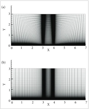
h e test case used in this work is the simulation of turbulent subsonic l ow over a l at plate geometry in absence of streamwise pressure gradients. h e work studies the addition of dif erent levels of artii cial dissipation, at dif erent distances of the wall, in an attempt to fully understand the ef ects of the high dissipative upwind spatial discretization over turbulent dimensionless boundary layer proi les and over the friction coei cient. All results are compared to analytical and experimental data. h e Mach number at the freestream condition is set to M∞ = 0.3, and the Reynolds number based on 1 m long l at plate is 7.2 million. h erefore, the l ow can be considered as a turbulent compressible l ow. h e computational domain covers a 3 m high and 7 m long region. h e wall l at plate is located between 3< x <4. As illustrated in Fig. 6, the applied boundary conditions are as follows: in the lower portion of the computational domain, symmetry is used between the entry and the l at plate, and between the trailing edge and the outlet; an adiabatic wall is assumed over the l at plate surface; and fari eld Riemann-type boundary conditions are used for all the other boundaries. h e simulations are performed using two grids, one with 60,000 cells and another with 210,000 cells, as illustrated in Fig. 7. Both meshes have y+ = 0.5 at the i rst grid point of the wall, but the mesh with 210,000 cells has more points near to the wall.
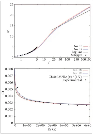
h e dimensionless boundary layer proi les obtained by the simulations are compared to the analytical formulation given by the law of wall (Schilichting, 1978), which is written by
y+< viscous sublayeru+= y+
30 5
< y+<300 log-law region u+= 1
0.41ln(y +
)+5.5 .
⎧ ⎨ ⎩
(114)
h e distribution of the local skin friction coei cient, cf , which is written as
cf=1 τw
2ρ∞u2∞
, (115)
is compared to experimental data (Coles and Hirst, 1969), and to the analytical formulation (von Karman, 1934) given by
cfvon Karman(Rex)=0.025Re
−1 7
x , (116)
3
2
1
0 3
2
1
0
0 1 2 3 4 5 6 7
0 1 2 3 4 5 6 7
Y
Y
X X (a)
(b)
Figure 7. Visualization of the meshes used in the zero-pressure-gradient l ow over a l at plate. (a) Mesh with 60,000 volumes; (b) Mesh with 210,000 volumes.
3
2
1
0 1
Symmetry Symmetry
F
ar
fie
ld
F
ar
fie
ld
Farfield
Wall
2 3 4 5 6 7
Y
X
where Rex is local Reynolds number based on a distance from the current position to a reference point, and is given by
Rex= ρU∞
x
µ , (117)
in which U∞ is the freestream velocity and x is the distance to a reference position.
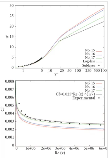
he upwind Steger-Warming (Steger and Warming, 1981) scheme is too dissipative and, therefore, implementing a turbulence closure to treat the turbulent lows is not enough to provide accurate results. he dissipative terms, present in the spatial discretization and in the turbulence model equations, need to be carefully treated. he efects of the spatial discretization on the results are analyzed by forcing the switch term, Eq. (24), to the classical Steger-Warming scheme, w = 0, and to the centered scheme, w = 0.5. he artiicial dissipation term, Eq. (25), and the Spalart-Allmaras cross-difusion-like term, Eq. (65), are added in diferent quantities and at diferent positions of the boundary layer proile in order to study their inluence on the skin friction coeicient and on the dimensionless boundary layer.
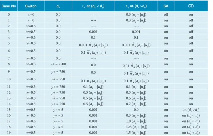
Table 1 presents the validation studies performed for this test case. It enumerates the simulations and indicates the chosen spatial discretization; the distance, d0, for the artiicial dissipation; the amount of artiicial dissipation at a given region; the choice of the turbulence model; and the choice of the cross-difusion-like term.
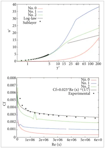
he irst three simulations are an introductory study of the numerical issues concerned in this work, and the results are illustrated in Fig. 8. Simulation No. 0 is performed without any turbulence modeling. It provides an underestimated cf distribution over the lat plate and a boundary layer proile completely diferent from the analytical turbulent one. For case No. 1, as an initial approximation, the cross-difusion-like term of the SA equation, the most expensive source term, is not included in the formulation and the inviscid lux is calculated using the original scheme of the code, as presented in Eqs. (23) and (24). he results with the turbulent model have shown to be better than those without any turbulence model. he boundary layer proile matches the analytical results at the viscous sublayer, however the excessive artiicial dissipation, provided from the spatial discretization, deteriorates the
Table 1. Zero-pressure-gradient low over lat plate simulations.
Case No Switch do
ϵ
k at (dk < do)ϵ
k at (dk >do) SA0 w=0 0.0 ---- 0.3 (ak + |uk|) of on
1 w=0 0.0 ---- 0.3 (ak + |uk|) on of
2 w=0.5 0.0 ---- ---- on of
3 w=0.5 0.0 0.001 0.001 on of
4 w=0.5 0.0 0.1 0.1 on of
5 w=0.5 0.0 0.001 →n
x (ax+ |ux|) 0.001 n →
x (ax+ |ux|)
on of
6 w=0.5 0.0 0.1 →n
x (ax+ |ux|) 0.1 n
→
x (ax+ |ux|)
on of
7 w=0.5 0.0 ---- ---- on on
8 w=0.5 y+ ≈ 7500 0.0 0.01 →n
x (ax+ |ux|)
on on
9 w=0.5 y+ ≈ 750 0.0 0.1 →n
x (ax+ |ux|)
on on
10 w=0.5 y+ ≈ 750 0.1 →n
x (ax+ |ux|) 0.1 n
→
x (ax+ |ux|)
on on
boundary layer proile at the log-law zone. he skin friction distribution is still underestimated, which indicates that the computation of shear-stress tensor, τw , at least at the wall, is not correct. Simulation No. 2 uses the centered scheme without any artiicial dissipation. he results present the same shortcomings as the previous ones discussed here. However, the results for test case No. 2 have shown to be closer to the analytical data.
he solution of a nonlinear partial diferential equation, spatially discretized without the addition of artiicial dissipation, is numerically unstable (Lomax et al., 2001), due to the frequency cascade phenomenon. Test case No. 2 achieved convergence of the solution because it provides a very simple geometry and due to the presence of the viscous luxes, which are dissipative by nature. he numerical solver set up, which uses the centered scheme without the addition of artiicial dissipation, is unstable and cannot be used for complex conigurations.
Simulations including test cases No. 3 to No. 19 are performed using the centered scheme. Artiicial dissipation is added to the formulation in diferent quantities, and at diferent locations within the boundary layer proile. he local error is measured as the diference between the analytical, and is given by
err(%)=100∗|LeM AN S−Analytical |
Analytical . (118)
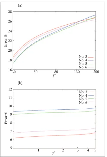
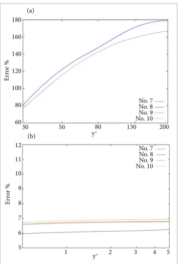
Figures 9 and 10 present the results and errors for simulations No. 3, 4, 5 and 6, using the SA model without the cross-difusion-like term. hese igures illustrate that the addition of artiicial dissipation, in the low direction, does not afect substantially the boundary layer proile. As with simulation No. 1, the results are in good agreement with the analytical ones at the sublayer zone and overpredicted the log-law zone by about 20% of the analytical value.
40
35
30
25
20
15
10
5
0
0.008
0.007
0.006
0.005
0.004
0.003
0.002
0.001
Cf
u
+
y+
Re (x) No. 0
No. 1 No. 2 Log-law Sublayer
No. 0 No. 1 No. 2 Cf=0.025*Re (x) ^(1/7) Experimental
1e+06 2e+06 3e+06 4e+06 5e+06 6e+0 1 5 10 15 25 40 65 100 200
00
Figure 8. Comparison of the dimensionless turbulent boundary layer and skin friction coeficient to analytical and experimental data (Coles and Hirst, 1969) for simulations 0, 1, and 2.
25
20
15
10
5
0
0.008
0.007
0.006
0.005
0.004
0.003
0.002
0.001
0
u
+
Cf
y+
Re (x)
No. 3 No. 4 No. 5 No. 6 Log-law Sublayer
No. 3 No. 4 No. 5 No. 6 Cf=0.025*Re (x) ^(1/7) Experimental
1e+06 2e+06 3e+06 4e+06 5e+06 6e+0 1 5 10 15 25 40 65 100 200
0