www.geosci-model-dev.net/7/2107/2014/ doi:10.5194/gmd-7-2107-2014
© Author(s) 2014. CC Attribution 3.0 License.
Improving subtropical boundary layer cloudiness
in the 2011 NCEP GFS
J. K. Fletcher1, C. S. Bretherton2, H. Xiao3, R. Sun4, and J. Han5 1Monash University, Clayton, Victoria, Australia
2University of Washington, Seattle, Washington, USA
3Pacific Northwest National Laboratory, Richland, Washington, USA 4IMSG at NOAA/NWS/NCEP/EMC, Camp Springs, Maryland, USA 5SRG at NOAA/NWS/NCEP/EMC, Camp Springs, Maryland, USA
Correspondence to:J. K. Fletcher ([email protected])
Received: 21 February 2014 – Published in Geosci. Model Dev. Discuss.: 9 April 2014 Revised: 6 August 2014 – Accepted: 6 August 2014 – Published: 23 September 2014
Abstract.The current operational version of National Cen-ters for Environmental Prediction (NCEP) Global Forecast-ing System (GFS) shows significant low cloud bias. These biases also appear in the Coupled Forecast System (CFS), which is developed from the GFS. These low cloud biases degrade seasonal and longer climate forecasts, particularly of short-wave cloud radiative forcing, and affect predicted sea surface temperature. Reducing this bias in the GFS will aid the development of future CFS versions and contributes to NCEP’s goal of unified weather and climate modelling.
Changes are made to the shallow convection and planetary boundary layer parameterisations to make them more con-sistent with current knowledge of these processes and to re-duce the low cloud bias. These changes are tested in a single-column version of GFS and in global simulations with GFS coupled to a dynamical ocean model. In the single-column model, we focus on changing parameters that set the fol-lowing: the strength of shallow cumulus lateral entrainment, the conversion of updraught liquid water to precipitation and grid-scale condensate, shallow cumulus cloud top, and the effect of shallow convection in stratocumulus environments. Results show that these changes improve the single-column simulations when compared to large eddy simulations, in particular through decreasing the precipitation efficiency of boundary layer clouds. These changes, combined with a few other model improvements, also reduce boundary layer cloud and albedo biases in global coupled simulations.
1 Introduction
The National Centers for Environmental Prediction (NCEP) Global Forecast System (GFS, http://www.emc.ncep.noaa. gov/GFS/doc.php) is an important model for operational weather forecasting. A frozen version of the GFS is coupled to the Modular Ocean Model v4 (http://www.gfdl.noaa.gov/ mom-ocean-model) and called the Coupled Forecast System (CFS); this is used for seasonal to inter-decadal climate pre-dictions and reanalyses (Saha et al., 2006, 2010). An out-standing problem for both the GFS and CFS, described in more detail below, is the representation of boundary layer clouds. We focus on improving parameterisation of these clouds and their associated processes in the GFS, using in-sights gained from parameterisation development work in climate models and studies using large eddy simulation.
It is anticipated that Version 3 of the CFS will be de-veloped from an upcoming operational version of the GFS, making current biases in the GFS relevant to forecasts of seasonal and longer timescales. Xiao et al. (2014) presented our CPT’s comparisons of the simulated climate from mul-tidecadal free-running simulations using an ocean-coupled version of the GFS operational in late 2011 with compara-ble simulations using Version 1 of the CESM (which uses the Community Atmosphere Model Version 5, or CAM5, as its atmospheric component). They found that the simu-lated GFS climatology was of comparable or higher quality to those with CESM1, except for cloud cover and radiative properties. The GFS-simulated global short-wave and long-wave cloud radiative effects were only about half as large as observed, with profound effects on the simulated planetary energy budget. Xiao et al. (2014) found that much of this re-sponse was attributable to inadequate cloud cover over most parts of the oceans, including the near-coastal part of the sub-tropical stratocumulus regions and sub-tropical–subsub-tropical shal-low cumulus regions. On the other hand, one of the few re-gions in which cloud cover and radiative effects were overes-timated in GFS is in the stratocumulus to cumulus transition regions, especially the East Pacific between the equator and 30◦S; the model fails to accurately represent the coastal/open ocean contrast in cloud cover in addition to an global mean low bias. Thus, by focusing on the simulation of boundary layer clouds in the eastern subtropical oceans, we also hope to improve GFS-simulated cloud climatology in many other regions and globally averaged cloud radiative properties.
One focal strategy of the CPT is to use benchmark single-column model tests to identify possible model improve-ments, which are then tested in short global integrations. This paper describes some initial efforts to implement this strategy for improving GFS cloud simulations.
2 Method
2.1 Model availability
We use GFS version 11.0.6 for both single-column and global model experiments. The GFS single-column model (SCM) used in this study, as well as the forcing files, can be downloaded at http://www.atmos.washington.edu/~jkf/ GFS_SCM.html, which also includes instructions for run-ning the SCM as well as routines modified for the ex-periments described in this paper. The global model may be downloaded at http://www.nco.ncep.noaa.gov/pmb/codes/ nwprod/sorc/global_fcst.fd/. The shallow convection and boundary layer scheme subroutines used in the single column model experiments are also available in the Supplement. 2.2 Single-column modelling
The SCM has proven a useful tool in testing general circu-lation model (GCM) physics on properties like clouds and
precipitation in isolation from the effects of large-scale cir-culations (Randall et al., 2003). GCM developers can use SCMs to compare model performance to that of high reso-lution models such as large eddy simulation (LES) by run-ning both with the same set of observationally derived forc-ings. These forcings specify the initial thermodynamic and wind profiles, the tendencies of these profiles over the course of the simulation, and either the sea surface temperature or the surface latent and sensible heat fluxes. As part of the GEWEX Cloud System Study (GCSS, now subsumed into the Global Atmospheric System Study or GASS), a rich set of forcing cases exists for this purpose, drawn from observa-tional field campaigns encompassing different environments ranging from nocturnal marine stratocumulus to continental deep convection (e.g. Siebesma et al., 2003; Stevens et al., 2005; Grabowski et al., 2006).
The GFS has seldom been subject to this type of testing in the past, with developers generally focusing on global model skill scores based on errors of meteorological variables such as 500 hPa heights. Investigations of GFS physics that have used the single-column modelling approach have been ori-ented toward cirrus clouds and ice phase microphysics (e.g. Luo et al., 2005). In single-column mode, we compare quan-tities relevant to the physics of warm boundary layer clouds, such as cumulus updraught mass flux and thermodynamic properties, to those of identically forced LES, using obser-vationally anchored cases. While single-column modelling cannot substitute for sensitivity tests using 3-D simulations, this method’s relative simplicity and comparability with LES makes it a useful tool for falsifying model physics and as a reference to guide interpretation of global model results.
Our approach thus far in using SCM to improve model physics has been to identify components of the parameterisa-tions most relevant to boundary layer clouds that are (a) for-mulated in ways that are inconsistent with current knowl-edge of the process in question and (b) possible sources of model bias. We then aim to improve the component of the scheme while maintaining the general framework of the pa-rameterisation. In other words, while, for example, the “dual mass flux” scheme of Neggers et al. (2009) is an attractive framework for unified parameterisation of large boundary layer eddies and shallow convection, to implement this in the GFS would require a complete overhaul of both the boundary layer and shallow convective schemes. Maintaining and im-proving the current framework is a more pragmatic approach to improving GFS physics in the short term. In some cases, sensitivity experiments comparing SCM to LES can identify sources of compensating errors, in which case simultaneous improvements must be made to several aspects of the physi-cal parameterisations to reduce simulation biases.
parameterised. SAM has been included in LES intercompar-ison studies for the GCSS cases used here (Siebesma et al., 2003; Stevens et al., 2005) and has been shown to repro-duce observed precipitation, liquid water path, surface fluxes and cloud fraction (where such observations are available) in those cases, except where we note otherwise.
2.3 Global model experiments
We also ran global model tests that complement our SCM experiments. Because global coupled-model experiments are far more computationally expensive than single-column ex-periments, we performed only three global exex-periments, with parameter changes chosen based partially on SCM re-sults and partially on simultaneous development strategies at NCEP.
As in Xiao et al. (2014), we use the NCAR Atmo-spheric Modeling Work Group/Working Group on Numer-ical Experimentation diagnostic package (http://www.cgd. ucar.edu/amp/amwg/diagnostics) to facilitate comparison of our global model experiments with observations.
3 Model overview
This study is based on the 2011 version of GFS, the same as that used in the single-column model. It has a spectral trian-gular truncation of 126 waves (T126), equivalent to roughly one degree horizontal grid spacing, and 64 hybrid sigma pressure levels (Sela, 2009). Compared with the previous version of the GFS, the main changes are in the parameterisa-tions of the shallow convection, the planetary boundary layer (PBL) and deep convection (Han and Pan, 2011). Features of these schemes are described in more detail in the next sec-tion.
This version of GFS uses the Atmospheric and Envi-ronmental Research Inc. Rapid Radiative Transfer Model (RRTM) long-wave parameterisation (Mlawer et al., 1997). The short-wave parameterisation is modified from the Na-tional Aeronautics and Space Administration (NASA) God-dard Space Flight Center solar radiation scheme (Hou et al., 2002; Chou et al., 1998). Both radiation schemes assume maximum random cloud overlap.
The microphysics scheme (Zhao and Carr, 1997; Moor-thi et al., 2001) prognoses cloud water specific humidity and cloud fraction following Sundqvist (1978). Both stratiform cloud processes and detrained cumulus cloud ice and con-densate are sources of total cloud water.
For the global simulations presented below, the GFS is coupled to the Modular Ocean Model 4 (MOM4), a finite difference version of the ocean primitive equations (Griffies et al., 2005). The zonal resolution is 1/2 degree. The merid-ional resolution gradually decreases from 1/4 degree near the equator to 1/2 degree at high latitudes. There are 40 height
layers, whose vertical spacing increases from 10 m near the surface to about 500 m in the bottom.
4 Physics parameterisations
This section summarises the GFS shallow convection, plan-etary boundary layer (PBL), and cloud fraction parameteri-sations, focusing on aspects relevant to our sensitivity tests. More detailed descriptions of these schemes are given by Troen and Mahrt (1986), Hong and Pan (1996) and Han and Pan (2011).
4.1 Shallow convection
The GFS shallow cumulus scheme (Han and Pan, 2011) is a bulk entraining plume mass flux parameterisation based on the GFS deep convection scheme (Pan and Wu, 1995; Han and Pan, 2011), but with new formulations of lateral entrain-ment and detrainentrain-ment rate, a different mass flux closure, and different plume microphysics.
The bulk plume originates from and shares the proper-ties of the level of highest moist static energy (MSE) in the boundary layer, usually the lowest model level. It rises to its lifted condensation level, where its mass flux is determined using the Grant (Grant and Brown, 1999) closure. The plume mass fluxmis given by the equation
1 m
dm
dz =ǫ−δ, (1)
whereǫis the fractional lateral entrainment rate andδ the fractional detrainment rate. The former is assumed to have the formǫ=c/z, where cis an adjustable nondimensional constant. The fractional detrainment rateδ is constant with height and equal to the fractional entrainment rate at the height of cloud base. This ensures a mass flux profile that decreases with height within the cumulus updraft, consistent with the LES study of Siebesma and Cuijpers (1995). It also means that changes tocaffect the detrainment rate as well as the entrainment rate. The same entrainment rate is used in de-termining the moist static energy and total water specific hu-midity (and hence the buoyancy) of the cumulus updraught, as well as its horizontal velocity, relevant for cumulus mo-mentum transport.
The bulk plume microphysics are simple: updraught liquid water is converted to precipitation (which falls down through the plume and can evaporate in the subcloud layer), and it is detrained to grid-scale cloud condensate, both at rates pro-portional to the updraught liquid water content, following Lord (1978):
qcprec∝c0qccu (2)
and
The scheme contains a flag that turns off shallow convection if the cloud top (constrained to a model level) is below the model-diagnosed PBL top, diagnosed with a bulk Richard-son number. This ensures that clouds that lack the buoyancy to penetrate the inversion are handled entirely by the PBL scheme rather than the shallow convection scheme. In the operational GFS, this flag is commented out because it has little impact on NCEP’s traditional forecast skill metrics. Our tests, discussed below, showed that this may nevertheless of-ten be important to the parameterised boundary-layer cloud cover and precipitation.
Shallow cumulus cloud top is determined by cloud work function (Arakawa and Schubert, 1974), i.e. the vertically in-tegrated buoyancy of the entraining updraught. Updraughts are given energy equal to 10 % of cloud work function to overshoot their level of neutral buoyancy. We test an alter-native formulation of cloud top that instead uses an equation for the square of the cumulus updraught vertical velocityw:
1 2
d(w2)
dz =aB−bǫw 2,
(4) where a and b are tunable parameters and B is the cu-mulus updraught buoyancy. Choosing the parameters such that b/a >1 roughly parameterises the effect of perturba-tion pressure gradients on vertical velocity (Bretherton et al., 2004).
Key parameters in the shallow convection scheme that affect its performance include the fractional entrain-ment/detrainment parameter cused in Eq. (1) and the rates c0andc1in Eqs. (2) and (3), respectively. If Eq. (4) is used to determine cloud top, thenaandb may also be important parameters.
4.2 PBL turbulence and stratiform clouds
The GFS boundary layer turbulence parameterisation (Hong and Pan, 1996) is an eddy diffusivity scheme modified from Troen and Mahrt (1986) with an added “countergradient” term (for temperature only) representing the nonlocal mixing done by the largest PBL eddies. Han and Pan (2011) modi-fied the turbulence scheme by adding a simple parameteri-sation of cloud-top-driven mixing after Lock et al. (2000). This entrainment rate is proportional to the radiative flux jump across cloud top and represents cloud top cooling en-hancement of boundary layer entrainment. The original Lock scheme also parameterised mixing-induced buoyancy rever-sal; this process is not included in the GFS scheme.
The operational GFS uses two different cloud fraction schemes: one for radiative flux calculations, the other for stratiform microphysics calculations. The radiation scheme uses the Xu and Randall (1996) fit of observed cloud fraction to relative humidity RH, condensate specific humidityql, and saturation specific humidityqs:
σXR=RHk1
1−exp
− k2ql [(1−RH)qs]k3
. (5)
The model uses the original Xu and Randall (1996) empirical values for the fit parameters:k1=0.25,k2=100,k3=0.49. However, the condensate specific humidity used is only that of the stratiform microphysics scheme. Thus, cumulus con-vection only interacts with radiation indirectly through its effect on large-scale temperature and moisture fields. The stratiform microphysics scheme is derived from Sundqvist (1978) and parameterises cloud fraction based on relative hu-midity in excess of a prescribed, latitudinally varying critical RH. The cloud fraction used in the Sundqvist scheme affects the model indirectly through the autoconversion and large-scale condensation rates. To maintain consistency with the rest of the scheme the Sundqvist formulation must be used. However, the Xu and Randall scheme matches observations better in general and is preferable for the radiation scheme. CPT members at NCEP are developing a single cloud frac-tion scheme to be used throughout the model in future GFS versions.
5 Single-column results 5.1 Model setup
The SCM is based on the operational version of the GFS, in-cluding the same 64 vertical levels, with vertical spacing in the PBL of 50–100 m. We run the SCM with a 5 min time step (half that used in the global simulations we present later in this paper), but the radiation scheme is called once per hour as in the GFS. In single-column mode, horizontal tendencies in wind, temperature, and moisture fields are prescribed by the forcing file in place of large-scale dynamics. The winds at each level are also forced by Coriolis and pressure gradient forces, taking the initial wind profile as the geostrophic wind. The SCM’s physical parameterisations are identical to those of the operational GFS except for options to include a few minor modifications planned for future GFS versions. These are discussed below and evaluated in our sensitivity exper-iments. Our single-column sensitivity tests use two GCSS cases, described below.
5.2 BOMEX
5.2.1 Experiment description
We use the BOMEX case to study model sensitivity to chang-ing aspects of the shallow convection scheme. In accordance with the discussion in Sect. 2.2, we test model sensitivity to changing several parameters. These parameter changes are summarised on Table 1. First, in theShCuCldCover experi-ment, we include cumulus updraught condensate in the cloud fraction parameterisation (Eq. 5). This change is included in subsequent experiments as well.
Second, we test sensitivity to the updraught lateral entrain-ment rate, parameterised as ǫ=c/z. We run experiments with LES-compatible choices of cin the range of 1.0–2.0 (Siebesma et al., 2003) instead of the operational valuec=
0.3. Because the GFS parameterises updraught detrainment rate as constant with height and equal to the entrainment rate at cloud base (where it is maximum within the cloud), chang-ingcalso changes the detrainment rate. For this reason, we will henceforth refer tocas the entrainment/detrainment pa-rameter.
At the same time, we test sensitivity to the efficiency of conversion of updraught condensate into precipitation or de-trained condensate. The operational GFS converts updraught condensate in a grid layer to precipitation and detrains it to grid-scale condensate at rates given in Eqs. (2) and (3); both rates are proportional to the condensate mixing ratio. This means that any updraught condensate is precipitated out over an e-folding depth of 400 m, causing extremely effi-cient precipitation even from the shallowest cumulus clouds. In practice, this compensates for the inadequate dilution of updraught condensate by lateral mixing, as we describe fur-ther below. In configuration NewEntr, we decreased these rates – in combination with increases to entrainment – to c0=0.001 m−1,c1=2.5×10⁻⁴m−1. This can be regarded as an intermediate step toward the LES results: inNewEntr
the lateral entrainment rate is still underestimated, compen-sated by overestimation of conversion of updraught con-densation to precipitation, but both compensating errors are much smaller than with the operational parameter choices.
Lastly, we also show the effect of using the vertical ve-locity Eq. (4) to determine cloud top. We show the effect of this change both without theNewEntrchange (VvelOrig) and with it (VvelNewEntr).
5.2.2 Results
Our initial sensitivity tests only involved single parameter changes. This quickly uncovered compensating errors – mul-tiple parameters incorrectly tuned such that their effects can-cel each other – in the shallow cumulus scheme. For exam-ple, only increasing the updraught lateral entrainment rate resulted in a simulation with an improved mass flux pro-file but far too small updraught condensate amount, while only decreasing the precipitation and detrainment conver-sion rates reduced excess precipitation but produced too
much condensate. Furthermore, only reducing one ofc0 or c1simply shifts precipitation between the shallow convection and stratiform microphysics schemes, with little reduction in overall precipitation. It is necessary to change all of these parameters together in order to address these compensating errors, so we only show results from simulations in which multiple parameters were changed.
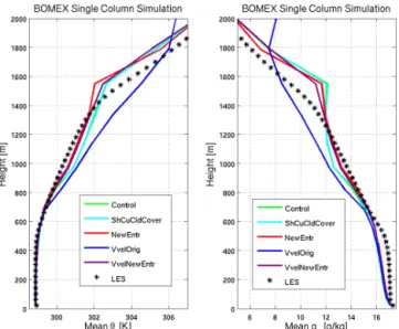
Figure 1 shows profiles of liquid water potential temper-ature and total water specific humidity averaged over hours 3–6 of the BOMEX experiments. We show these primarily to give the reader a sense of the environment being simu-lated: a fairly well-mixed subcloud layer up to about 500 m, a conditionally unstable cloud layer, and a capping inversion starting slightly above 1400 m. SCM results differ from LES primarily in a less well-mixed subcloud layer, a more stably stratified cloud layer, and excess moisture at the inversion. This last feature is explored more in the forthcoming discus-sion. Biases are most extreme in theVvelOrigconfiguration, with profiles that imply far too much mixing with the free troposphere.
A major problem with the control GFS simulation of the BOMEX case is that it over-precipitates. The BOMEX case is idealised, but it is designed to mimic a several-day pe-riod during which observers and photographs suggest pre-cipitation was negligible (Siebesma and Cuijpers, 1995), consistent with our LES results. Figure 2a shows time se-ries of surface precipitation for the experiments. The con-trol configuration maintains a convective precipitation rate of
∼1.5 mm day−1, large enough to be a sizable moisture sink to the trade cumulus boundary layer, compensating roughly 30 % of the surface evaporation.NewEntrreduces the con-vective precipitation by 60 %, but does not eliminate the problem because the precipitation flux is still proportional to the updraught condensate specific humidity, ensuring that all shallow convection will precipitate at least a little.
The VvelOrig configuration actually worsens the bias. Later we show that this is due to an overdeepening of cu-mulus convection. However, in combination withNewEntr, the spurious precipitation is reduced and the shallow convec-tion scheme is prevented from switching off and on as it does in the non-Vvelexperiments.
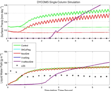
Figure 2 shows that all configurations maintain very small liquid water path (LWP) for the first few hours of simula-tion. This is because nearly all the cloud water is associ-ated with the shallow convection scheme. At varying times in the simulation, however, the LWP rapidly increases in the
Control,ShCuCldCoverandNewEntrexperiments. This in-dicates rapid development of stratiform cloud, which only theVvelchange is able to prevent.
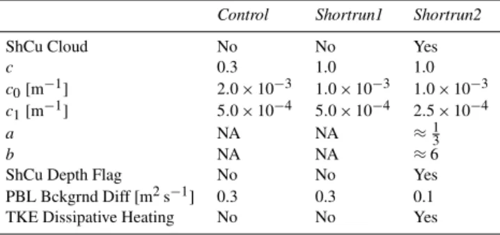
Table 1.Parameter settings for SCM experiments with the BOMEX shallow convection cases. Parametersaandbrefer to coefficients in Eq. (4).
Control ShCuCldCover NewEntr VvelOrig VvelNewEntr
ShCu cloud No Yes Yes Yes Yes
c 0.3 0.3 1.0 0.3 1.0
c0[m−1] 2.0×10⁻³ 2.0×10⁻³ 1.0×10⁻³ 2.0×10⁻³ 1.0×10⁻³ c1[m−1] 5.0×10⁻⁴ 5.0×10⁻⁴ 2.5×10⁻⁴ 5.0×10⁻⁴ 2.5×10⁻⁴
a NA NA NA ≈13 ≈13
b NA NA NA ≈6 ≈6
Figure 1.BOMEX liquid water potential temperature (left) and to-tal water (right) profiles averaged over hours 3–6. Coloured lines are different SCM experiments; black stars are LES.
that simply adding cumulus condensate to the radiation cloud fraction – theShCuCldCoverchange – is a major improve-ment, though the bias is now too much cloud cover rather than too little. This bias is reduced by subsequent parameter changes, and the spike in upper PBL cloud cover (and con-densate) is removed by theVvelchange. Finally, comparing the middle and right panels shows the large difference that can exist between cloud fraction in the microphysics scheme and that of the radiation scheme.
Figure 4 shows time-averaged cumulus updraught proper-ties: mass flux and condensate specific humidity. For the LES comparison, we define cumulus updraught properties as the average across all LES grid points that are both saturated and have positive vertical velocity.
The mass flux profiles of theControlandShCuCldCover
configurations show the effect of those experiments’ high precipitation. Evaporation of rainfall below cloud base over-stabilises the subcloud layer, reducing cumulus updraught buoyancy such that convection often extends only one or two grid levels above cloud base – if it is not shut off completely.
Figure 2.BOMEX time series of surface precipitation rate (top) and liquid water path (bottom) in the first 6 h of simulation. Coloured lines are different SCM experiments; black stars are LES.
This leads to a time-averaged mass flux profile that is too bottom-heavy and biased low, particularly between 800 and 1200 m. However, the cloud top is in good agreement with LES.
TheNewEntr parameter change improves on this by re-ducing precipitation directly (via the precipitation efficiency c0) and indirectly (via increased entrainment dilution and re-duced mass flux in the upper cloud layer). However, the cloud top is lower than theControlconfiguration and LES – this is also due to increased entrainment dilution. The tendency of the GFS to produce too-low shallow cumulus cloud top when the entrainment rate is set to a value suggested by cur-rent knowledge is in fact why the operational value ofcis so small.
TheVvelparameter change increases cloud depth and en-hances penetrative entrainment of warm dry inversion air. This is what prevents stratiform condensation in the Vvel
Figure 3.BOMEX grid-scale condensate (left, g kg−1) and cloud fraction as calculated in the stratiform microphysics (centre) and radiation (right) parameterisations, averaged over hours 3–6. Coloured lines are different SCM experiments; black stars are LES.
improvement in the mass flux profile – as well as those shown in previous figures – is seen.
Finally, the right panel of Fig. 4 demonstrates the com-pensating errors at work in the shallow convection scheme. All configurations produce similar values for cumulus up-draught condensate specific humidity, values that are close to that of LES. They do so via different tradeoffs between pre-cipitation and entrainment. A major aspect of our parameter changes has aimed to shift the removal of updraught liquid water content away from precipitation and toward increased mixing with the free troposphere.
5.3 DYCOMS
To study model behaviour in a stratocumulus environment, we use a case distilled from the Dynamics and Chemistry of Marine Stratocumulus (DYCOMS-II, referred to hereafter as DYCOMS) Research Flight 1, which sampled a nocturnal, nonprecipitating, well-mixed marine stratocumulus bound-ary layer under a strong capping inversion in the Northeast Pacific (Stevens et al., 2003). We use the GCSS DYCOMS case forcings as presented by Stevens et al. (2005) and Zhu et al. (2005). However, those studies used an idealised long-wave radiation code in their simulations; we use the full model (long-wave only) radiation code in both SCM and LES.
5.3.1 Experiment description
We found in ourControlDYCOMS simulation that the shal-low cumulus scheme was transporting much of the heat and moisture through the PBL despite this being a stratocumulus case (not shown). Recall from Sect. 4.1 that there is a logi-cal flag within the shallow convection scheme code that turns shallow convection off if the cumulus cloud top is at or below PBL top. Thus, in boundary layers where moist updraughts have insufficient energy to penetrate the capping inversion, PBL cloudiness and entrainment will be handled by the PBL
Figure 4.BOMEX shallow cumulus updraught (left) mass flux and (right) condensate profiles averaged over hours 3–6. Coloured lines are different SCM experiments; black stars are LES.
scheme rather than the cumulus convection scheme. This flag is not used by default, even though it is physically reason-able, but we experimented with using it, effectively turning convection off for the duration of the run. This “ShCuFlag” experiment is shown along with the configurations already shown for the BOMEX case. The exception to this is the
ShCuCldCoverconfiguration, which has no effect on the DY-COMS case and is not shown here.
The operational GFS also includes a minimum back-ground diffusion applied both in and above the PBL. The background diffusivity for heat and moisture in the op-erational GFS decreases exponentially with height from 1.0 m2s−1, giving rise to about 0.9 m2s−1 at the 900 hPa level, a typical PBL top in marine stratocumulus. To reduce erosion of coastal stratocumulus, NCEP developers have fur-ther reduced the lower inversion layers’ background diffu-sivity; it is now 30 % of that at the surface (i.e. 0.3 m2s−1; Han and Pan, 2011). Hence, we use this reduced background diffusivity in our DYCOMS simulations.
5.3.2 Results
All DYCOMS experiments with the GFS maintain a reason-ably strong capping inversion, given the model resolution, and produce cloud fraction of about 1.0 after initial spinup (not shown). In this respect, the DYCOMS SCM simulations do not have the same biases that the global coupled model shows in the Northeast Pacific, where the model generates too shallow boundary layer and too low cloud fraction. This limits the interpretation of SCM results.
Figure 5.DYCOMS time series of surface precipitation rate (top) and liquid water path (bottom) in the first 6 h of simulation. Coloured lines are different SCM experiments; black stars are LES. Results are identical for all experiments without shallow convec-tion, thus ShCuFlag and VvelOrig are hidden by VvelNewEntr.
to be about 60 g m−2. The SCM LWP is actually closer to observations. However, this is achieved with a drizzle rate of roughly 0.5 mm d−1. Both observations (Stevens et al., 2003) and LES indicated no drizzle at the surface or even at cloud base. Thus it appears that, as with the convection scheme, the physics parameterisations controlling stratocumulus are too tuned toward precipitation as a mechanism for PBL dry-ing. The simplest explanation is that the modified Lock et al. (2000) parameterisation in the SCM is not producing enough cloud top entrainment of warm, dry air. Initial results, to be reported in a future study, indicate that increasing the entrain-ment rate in the Lock scheme while simultaneously decreas-ing the autoconversion rate in the stratiform microphysics scheme can maintain observed LWP while reducing excess precipitation in the DYCOMS simulation.
The most obvious differences are between (1) theControl
and NewEntr experiments, and (2) the ShCuFlag andVvel
experiments. As part of the implementation of using verti-cal velocity for cloud top prediction, a logiverti-cal flag turning off shallow convection if it is less than 70 hPa deep is in-cluded. Thus, theVvelconfigurations look just like the ShCu-Flag configuration because all of them result in the model turning off shallow convection. Figure 5 shows that, with-out shallow convection, the model takes ∼2.5 h to spin up cloud LWP despite having a 5 min time step and having been initialised with a supersaturated moisture profile. However, experiments with a different stratocumulus case (not shown) show that this is not the case if the model is initialised with liquid water, and furthermore initialising with liquid water eliminates the oscillations that are seen when the shallow convection scheme is active. These oscillations result from
convective precipitation stabilising the subcloud layer and re-ducing convective mass flux, and hence detrained convective condensate, in the subsequent time step.
6 Global model results
6.1 Configuration and experiment description
We perform four simulations with the global version of GFS coupled to MOM4: a 50-year run with GFS operational set-tings; a 1-year control run that, apart from length, is identical to the 50 year run; and two 1-year sensitivity experiments: shortrun1 and shortrun2.Shortrun1includes most of the pa-rameter changes to the shallow convection scheme suggested by our BOMEX SCM study.Shortrun2also includes changes suggested by the DYCOMS study and by basic physical considerations not exposed by either SCM case. All exper-iments are identically initialised on 1 January 1948. The at-mosphere is initialised by NCEP-NCAR reanalysis (Kalnay et al., 1996); the ocean is initialised with the Climate Forecast System Reanalysis (Saha et al., 2010), and the initial state is neutral with respect to the NINO3.4 (El Niño/Southern Os-cillation) index. We included ocean coupling for two reasons. First, it corresponds to the setup for seasonal climate predic-tion, an important application of GFS. Second, it was eas-ier for us to set up a coupled simulation than an uncoupled simulation with seasonally varying sea surface temperatures (SSTs).
The parameter changes in Shortrun1and Shortrun2 are summarised in Table 2.Shortrun1increases the lateral en-trainment rate and reduces the rain conversion rate in the shallow convection parameterisation, following two of the three prescriptions in the BOMEXNewEntrcase.Shortrun2
also reduces the condensate detrainment rate (the other pa-rameter change made inNewEntr), uses cumulus condensate for cloud fraction, and uses the vertical velocity Eq. (4) for cloud top.Shortrun2also incorporates the additional changes discussed in the DYCOMS ShCuFlag case – to prevent shal-low convection with a cloud top that does not extend above the PBL top and to decrease background diffusion in inver-sion layers. However, the former might have little impact in combination with the vertical velocity cloud top change, as was seen in the DYCOMS simulations.
Table 2.Parameter settings for free-running coupled global model experiments.
Control Shortrun1 Shortrun2
ShCu Cloud No No Yes
c 0.3 1.0 1.0
c0[m−1] 2.0×10⁻³ 1.0×10⁻³ 1.0×10⁻³ c1[m−1] 5.0×10⁻⁴ 5.0×10⁻⁴ 2.5×10⁻⁴
a NA NA ≈13
b NA NA ≈6
ShCu Depth Flag No No Yes
PBL Bckgrnd Diff [m2s−1] 0.3 0.3 0.1
TKE Dissipative Heating No No Yes
be presented in a forthcoming paper; they have little effect on subtropical boundary layer clouds.
For the following discussion we focus on marine low cloud sensitivity in the southeastern Pacific for September– October–November (SON). Even though this is only 9– 11 months after the start of the simulations, the climatolog-ical marine low cloud bias and its sensitivity to parameter changes has already emerged, as can be seen by comparing Fig. 6a (the 1-year run) and 6d (the 50-year run). Cloudi-ness differences driven by synoptic timescale variability in the southeastern Pacific may affect the exact magnitudes of changes in the bias in the sensitivity experiments; by com-paring the differences between the simulations in the three individual months comprising the SON period (not shown) we are confident that the signals we report are robust to syn-optically driven cloudiness fluctuations.
6.2 Results
Figures 6 and 7 show the sensitivity of short-wave cloud ra-diative effect (SWCRE) and low cloud fraction over the Pa-cific region for SON. In these plots, panel a shows the bias of the control simulation compared to satellite-derived clima-tologies, and the next two panels show the difference of the control from the two sensitivity runs. The observations used in Fig. 7a are a combination of the climatological low cloud fraction from the CLOUDSAT/CALIPSO GEOPROF prod-uct (Kay and Gettelman, 2009) and the CALIPSO GOCCP product (Chepfer et al., 2010) for 2006–2010 – in each grid box the maximum low cloud fraction from the two is used. This method enhances the low cloud fraction just off the west coasts of the American and African continents because GEO-PROF tends to underestimate low cloud amount because it screens out clouds with tops below 500 m altitude. However, GEOPROF is more accurate in general because the combi-nation of CLOUDSAT and CALIPSO instruments can de-tect low clouds better when mid- and high-level clouds are present. The SWCRE observation used in Fig. 6a and d is from the Clouds and Earth’s Radiant Energy System Edition 2 (CERES2, Minnis et al., 2011) for 2000–2005. In these panels, biases on the Controlsimulation are reduced where
Figure 6.Short-wave cloud forcing biases and their improvements in global simulations. Panel(a)shows the bias in the control run compared to observations; panel(b)shows the difference between control and shortrun1; panel(c)shows the difference between con-trol and shortrun2. In panels(b)and(c), the respective experiment bias has been eliminated to the extent that the pattern matches(a). See text for further explanation. Panel(d)shows the bias in the 50-year control run.
the colours indicate differences of the same sign as the upper panel (e.g. blue colours where there is a blue colour in the upper panel, or vice versa).
While it would be ideal to compare model simulations to observations over the same time period, we found it techni-cally much simpler to initialise the short GFS runs with the same initial conditions as the 50-year run rather than with initial conditions from the satellite era. Long-term trends and decadal variability in global mean downwelling surface ra-diation are of the order of+0.25 and±3–5 W m−2, respec-tively (Hinkelman et al., 2009), one to two orders of magni-tude smaller than the GFS short-wave bias. Additionally, the decade 2000–2010 was one of weak El Niño–Southern Oscil-lation variability (http://www.esrl.noaa.gov/psd/enso/mei/). This gives us confidence that the difference in decades for which we compare means will not substantially affect our results.
Figure 7.Cloud fraction bias and its improvement in global sim-ulations. Panel (a)shows the bias in the control run compared to observations; panel (b)shows the difference between control and shortrun1; panel(c)shows the difference between control and short-run2. In panels(b)and(c), the respective experiment bias has been eliminated to the extent that the pattern matches(a). See text for further explanation.
inShortrun2, which we will discuss in more detail together with the SST response later in this section. The global mean SWCRE bias in Shortrun2, compared to that inControl, is reduced by about half, from∼23 to∼11 W m−2for the an-nual average of 1948 minus the CERES2 anan-nual mean from 2000 to 2005; this bias reduction occurs persistently through-out the year.
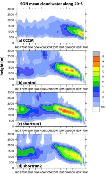
Figure 8 shows the sensitivity of low cloud structure along 20◦S in the East and Central Pacific for SON. In Control
(Fig. 8b), the lack of clouds near the coast and the overexten-sion offshore is clear in comparison to the CERES2-MODIS-CALIPSO-CLOUDSAT (CCCM) data set from the Atmo-spheric Science Data Center at NASA Langley Research Center, Fig. 8a.
Figure 8.Cloud condensate along the 20 S Pacific cross section in (a)observations,(b)the control run,(c)shortrun1 and(d) short-run2.
Figure 9.Shallow cumulus heating (left column) and moistening (right column) in the control run (top), shortrun1 (middle) and shortrun2 (bottom).
The cloud structure changes can be related to changes in the behaviour of the parameterised shallow convection. Fig-ure 9 shows heating and moistening from the shallow con-vection scheme in each experiment along the transect. The difference betweenShortrun2andShortrun1east of 100◦W shows that nearly all shallow convective activity has been eliminated in this region, which is observed to be dominated by stratocumulus clouds. Meanwhile, increasing the entrain-ment/detrainment parameter (one of the two differences be-tweenShortrun1andControl) decreases mass flux in the up-per cloud layers and thus reduces convective heating in the cumulus and Sc–Cu transition regions west of 100◦W.
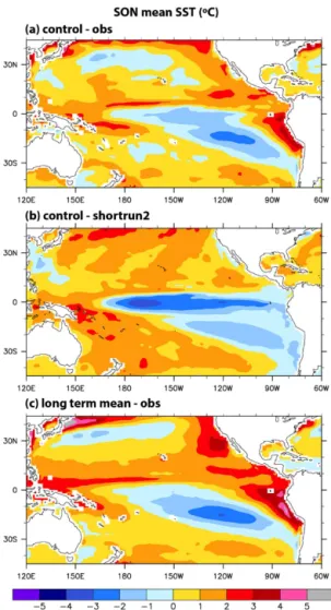
The SST response in SON is shown in Fig. 10 for Short-run2. The response inShortrun1is small and not shown here. InControl, we see large positive SST errors near the Ameri-can coasts (4◦C off South American coast) and negative bi-ases to their west (−2◦C in the southeastern Pacific). In the tropics, there are warm SST biases of 2◦C along the ITCZ and SPCZ and near the maritime continent, and negative bi-ases along the equator. In Shortrun2, the negative biases in the southeastern Pacific are reduced by at least half but the warm biases near the coast are worsened. In the tropics the warm biases along ITCZ and SPCZ and near the maritime continent are reduced, but the equatorial cold bias is turned into a warm bias, especially between 150 and 180◦W.
It is unlikely that changes in cloud radiative forcing di-rectly caused the SST changes in deep convective regions,
where the substantial change in short-wave cloud forcing was largely offset by a change in long-wave cloud forcing (not shown). However, reductions in excess cloud cover in the off-shore southeast Pacific may contribute to the increase in SST in that region and subsequent reduction in zonal SST gradient associated with a weakening of the Walker circulation. This can also be seen in the change in SST off the Peruvian and Chilean coasts, where positive SST biases worsen despite an increase in cloud cover. This is likely due to a weakening in coastal upwelling. We found that changes in wind stress also suggest a weakening of this circulation, with a decrease in surface easterlies in the central and west Pacific and a reduc-tion of northerlies in the southeast Pacific (not shown). Such sensitivity of the basin-wide Hadley–Walker circulation pat-tern to changes in marine low clouds associated with param-eter changes in shallow convection and moist turbulence pa-rameterisation is also found in other GCMs (e.g. Ma et al., 1994; Xiao et al., 2014).
7 Future tests
Figure 10.Pacific SST in global simulations:(a)bias in the control run;(b)the difference between control and shortrun2, and(c)bias in the 50 year control run. In panel(b), the experiment has eliminated the bias to the extent that the pattern matches that of panel(a). See text for further explanation.
especially in terms of the 500 hPa anomaly correlation, pre-cipitation skill over the United States, or hurricane track fore-cast, the change is likely to be implemented. If the skill is neutral but the climate bias is reduced, there is still a good chance of implementing the change. If the forecast skill is degraded, modifications or re-tuning of other model param-eters, such as those controlling autoconversion or the critical relative humidity used for condensation, will be tried.
A short data assimilation experiment implementing the model changes included in theNewEntrandShCuCldCover
SCM results of BOMEX and DYCOMS, respectively, has been performed. Initial results suggest that, while in many respects the forecast skill is improved or neutral, the root mean square error in tropical horizontal winds is increased. As a consequence of these experiments, further work must be done before these changes can be implemented into fu-ture versions of the GFS; climate improvements must, at the
very least, have a neutral impact on forecasts. Single col-umn tests (not shown) indicate that changes in horizontal winds are not a result of cumulus momentum transport – the
NewEntr change has no impact on winds in the SCM. In-stead, the change is affecting horizontal pressure gradients; thus more global model tests – and possible model retuning – are needed to investigate this further. This work is under-way by NCEP developers and will be reported on in a future study.
8 Conclusions
The NOAA stratocumulus-to-cumulus transition Climate Process Team has run sensitivity experiments to single-column and global coupled versions of the NCEP-GFS model in conjunction. To improve the GFS simulation of sub-tropical boundary layer cloud, we used single-column simu-lations to identify and attribute underlying problems in the shallow convection scheme, and we then tested improve-ments suggested by this approach in short global coupled simulations.
In single-column mode, we found that some simple pa-rameter changes to the shallow convection scheme improved simulated boundary layer structure and precipitation com-pared to LES. In particular, it is beneficial to increase cu-mulus lateral mixing with the environment and decrease the rate at which updraught condensate falls out as rain and is detrained to the grid scale. This shifts some of the cumulus updraught removal of water from precipitation to evaporation associated with entrainment.
However, the single-column model still over-precipitates in both shallow convective and stratiform environments. We hypothesise that this can be improved by increasing entrain-ment of warm, dry free-tropospheric air into the boundary layer through changes to the boundary layer scheme, by re-ducing autoconversion of liquid cloud water to rain in the stratiform microphysics scheme, and by reformulating shal-low convective precipitation to suppress all rainfall when condensate specific humidity is small.
One-year global coupled model experiments combining these changes substantially reduce biases in subtropical low cloud fraction and short-wave cloud forcing seen in the trol version of GFS. Improvements are seen in the deep con-vective regions as well as the subtropical boundary layer cloud regimes. Global model changes also improve SST and precipitation bias in most regions. However, underestimation of low cloud off the subtropical west coasts of the Ameri-cas remains a problem even after the changes, and increased tropical wind RMSE must be addressed before this change can be implemented in the GFS.
global cloud cover and its radiative effects through improve-ments of the microphysics, cloud fraction, cumulus convec-tion, and PBL parameterisations and their interactions.
The Supplement related to this article is available online at doi:10.5194/gmd-7-2107-2014-supplement.
Acknowledgements. This work is supported by NOAA MAPP grant GC10-670a as part of the Sc–Cu Climate Process Team. The first author would like to thank Hua-Lu Pan at NCEP for his support and Peter Blossey at University of Washington for providing LES runs.
Edited by: J. C. Hargreaves
References
Arakawa, A. and Schubert, W. H.: Interaction of a
cu-mulus cloud ensemble with the large-scale
environ-ment, J. Atmos. Sci., 31, 674–701, doi:10.1175/1520-0469(1974)031<0674:ioacce>2.0.co;2, 1974.
Bister, M. and Emanuel, K. A.: Dissipative heating and hurricane intensity, Meteorol. Atmos. Phys., 65, 233–240, 1998.
Bretherton, C. S., McCaa, J. R., and Grenier, H.: A new param-eterization for shallow cumulus convection and its application to marine subtropical cloud-topped boundary layers. Part I: De-scription and 1D results, Mon. Weather Rev., 132, 864–882, doi:10.1175/1520-0493(2004)132<0864:anpfsc>2.0.co;2, 2004. Chepfer, H., Bony, S., Winker, D., Cesana, G., Dufresne, J. L., Min-nis, P., Stubenrauch, C. J., and Zeng, S.: The GCM-Oriented CALIPSO Cloud Product (CALIPSO-GOCCP), J. Geophys. Res.-Atmos., 115, D00H16, doi:10.1029/2009jd012251, 2010. Chou, M. D., Suarez, M. J., Ho, C. H., Yan, M. M. H., and
Lee, K. T.: Parameterizations for cloud overlapping and short-wave single-scattering properties for use in general circula-tion and cloud ensemble models, J. Climate, 11, 202–214, doi:10.1175/1520-0442(1998)011<0202:pfcoas>2.0.co;2, 1998. Grabowski, W. W., Bechtold, P., Cheng, A., Forbes, R., Halli-well, C., Khairoutdinov, M., Lang, S., Nasuno, T., Petch, J., Tao, W. K., Wong, R., Wu, X., and Xu, K. M.: Daytime con-vective development over land: A model intercomparison based on LBA observations, Q. J. Roy. Meteorol. Soc., 132, 317–344, doi:10.1256/qj.04.147, 2006.
Grant, A. L. M. and Brown, A. R.: A similarity hypothesis for shallow-cumulus transports, Q. J. Roy. Meteorol. Soc., 125, 1913–1936, doi:10.1256/smsqj.55801, 1999.
Griffies, S. M., Gnanadesikan, A., Dixon, K. W., Dunne, J. P., Gerdes, R., Harrison, M. J., Rosati, A., Russell, J. L., Samuels, B. L., Spelman, M. J., Winton, M., and Zhang, R.: Formulation of an ocean model for global climate simulations, Ocean Sci., 1, 45–79, doi:10.5194/os-1-45-2005, 2005.
Han, J. and Pan, H.-L.: Revision of Convection and Vertical Dif-fusion Schemes in the NCEP Global Forecast System, Weather Forecast., 26, 520–533, doi:10.1175/waf-d-10-05038.1, 2011.
Hinkelman, L. M., Stackhouse Jr., P. W., Wielicki, B. A., Zhang, T., and Wilson, S. R.: Surface insolation trends from satellite and ground measurements: Comparisons and challenges, J. Geophys. Res., 114, 1–18, doi:10.1029/2008JD011004, 2009.
Holland, J. Z. and Rasmusson, E. M.: Measurements of atmo-spheric mass, energy, and momentum budgets over a 500-kilometer square of tropical ocean, Mon. Weather Rev., 101, 44– 55, doi:10.1175/1520-0493(1973)101<0044:motame>2.3.co;2, 1973.
Hong, S. Y. and Pan, H. L.: Nonlocal boundary layer
ver-tical diffusion in a Medium-Range Forecast Model,
Mon. Weather Rev., 124, 2322–2339, doi:10.1175/1520-0493(1996)124<2322:nblvdi>2.0.co;2, 1996.
Hou, Y., Moorthi, S., and Compana, K.: Parameterization of so-lar radiation transfer in NCEP models, NCEP Office Note, #441, available at: http://www.emc.ncep.noaa.gov/officenotes/ FullTOC.html#2000, 2002.
Kalnay, E., Kanamitsu, M., Kistler, R., Collins, W., Deaven, D., Gandin, L., Iredell, M., Saha, S., White, G., Woollen, J., Zhu, Y., Chelliah, M., Ebisuzaki, W., Higgins, W., Janowiak, J., Mo, K. C., Ropelewski, C., Wang, J., Leetmaa, A., Reynolds, R., Jenne, R., and Joseph, D.: The NCEP/NCAR 40-year reanalysis project, B. Am. Meteorol. Soc., 77, 437–471, doi:10.1175/1520-0477(1996)077<0437:tnyrp>2.0.co;2, 1996.
Kay, J. E. and Gettelman, A.: Cloud influence on and response to seasonal Arctic sea ice loss, J. Geophys. Res.-Atmos., 114, D18204, doi:10.1029/2009JD011773, 2009.
Khairoutdinov, M. F. and Randall, D. A.: Cloud resolving mod-eling of the ARM summer 1997 IOP: Model formulation, re-sults, uncertainties, and sensitivities, J. Atmos. Sci., 60, 607–625, doi:10.1175/1520-0469(2003)060<0607:crmota>2.0.co;2, 2003. Lock, A. P., Brown, A. R., Bush, M. R., Martin, G. M., and Smith, R. N. B.: A new boundary layer mixing scheme. Part I: Scheme description and single-column model tests, Mon. Weather Rev., 128, 3187–3199, doi:10.1175/1520-0493(2000)128<3187:anblms>2.0.co;2, 2000.
Lord, S.: Development and observational verification of cumulus cloud parameterization, Ph. D. Thesis, University of California, Los Angeles, 1978.
Luo, Y. L., Krueger, S. K., and Moorthi, S.: Cloud properties sim-ulated by a single-column model. Part I: Comparison to cloud radar observations of cirrus clouds, J. Atmos. Sci., 62, 1428– 1445, doi:10.1175/jas3425.1, 2005.
Ma, C. C., Mechoso, C. R., Arakawa, A., and Farrara, J. D.: Sen-sitivity of a coupled ocean-atmosphere model to physical pa-rameterizations, J. Climate, 7, 1883–1896, doi:10.1175/1520-0442(1994)007<1883:soacom>2.0.co;2, 1994.
Mlawer, E. J., Taubman, S. J., Brown, P. D., Iacono, M. J., and Clough, S. A.: Radiative transfer for inhomogeneous atmospheres: RRTM, a validated correlated-k model for the longwave, J. Geophys. Res.-Atmos., 102, 16663–16682, doi:10.1029/97jd00237, 1997.
Trans-port, J. Atmos. Sci., 66, 1465–1487, doi:10.1175/2008jas2635.1, 2009.
Pan, H. and Wu, W.: Implementing a mass flux convective pa-rameterization package for the NMC Medium- Range Fore-cast model, NMC Office Note, 409, available at: http://www. emc.ncep.noaa.gov/officenotes/FullTOC.html#1990 (last access: 9 September 2014), 1995.
Randall, D., Krueger, S., Bretherton, C., Curry, J., Duynkerke, P., Moncrieff, M., Ryan, B., Starr, D., Miller, M., Rossow, W., Tse-lioudis, G., and Wielicki, B.: Confronting models with data – The GEWEX cloud systems study, B. Am. Meteorol. Soc., 84, 455–469, doi:10.1175/bams-84-4-455, 2003.
Saha, S., Nadiga, S., Thiaw, C., Wang, J., Wang, W., Zhang, Q., Van den Dool, H. M., Pan, H. L., Moorthi, S., Behringer, D., Stokes, D., Pena, M., Lord, S., White, G., Ebisuzaki, W., Peng, P., and Xie, P.: The NCEP Climate Forecast System, J. Climate, 19, 3483–3517, doi:10.1175/jcli3812.1, 2006.
Saha, S., Moorthi, S., Pan, H.-L., Wu, X., Wang, J., Nadiga, S., Tripp, P., Kistler, R., Woollen, J., Behringer, D., Liu, H., Stokes, D., Grumbine, R., Gayno, G., Wang, J., Hou, Y.-T., Chuang, H.-Y., Juang, H.-M. H., Sela, J., Iredell, M., Treadon, R., Kleist, D., Van Delst, P., Keyser, D., Derber, J., Ek, M., Meng, J., Wei, H., Yang, R., Lord, S., Van den Dool, H., Kumar, A., Wang, W., Long, C., Chelliah, M., Xue, Y., Huang, B., Schemm, J.-K., Ebisuzaki, W., Lin, R., Xie, P., Chen, M., Zhou, S., Higgins, W., Zou, C.-Z., Liu, Q., Chen, Y., Han, Y., Cucurull, L., Reynolds, R. W., Rutledge, G., and Goldberg, M.: The NCEP climate fore-cast system reanalysis, B. Am. Meteorol. Soc., 91, 1015–1057, doi:10.1175/2010bams3001.1, 2010.
Sela, J.: Implementation of the sigma pressure hybrid coordinate into GFS, Tech. rep., NCEP office Note, 2009.
Siebesma, A. P. and Cuijpers, J. W. M.: Evaluation of
parametric assumptions for shallow cumulus
convec-tion, J. Atmos. Sci., 52, 650–666, doi:10.1175/1520-0469(1995)052<0650:eopafs>2.0.co;2, 1995.
Siebesma, A. P., Bretherton, C. S., Brown, A., Chlond, A., Cuxart, J., Duynkerke, P. G., Jiang, H. L., Khairoutdinov, M., Lewellen, D., Moeng, C. H., Sanchez, E., Stevens, B., and Stevens, D. E.: A large eddy simulation intercomparison study of shallow cumulus convection, J. Atmos. Sci., 60, 1201–1219, doi:10.1175/1520-0469(2003)60<1201:alesis>2.0.co;2, 2003.
Stevens, B., Lenschow, D. H., Vali, G., Gerber, H., Bandy, A., Blomquist, B., Brenguier, J. L., Bretherton, C. S., Burnet, F., Campos, T., Chai, S., Faloona, I., Friesen, D., Haimov, S., Laursen, K., Lilly, D. K., Loehrer, S. M., Malinowski, S. P., Morley, B., Petters, M. D., Rogers, D. C., Russell, L., Savic-Jovac, V., Snider, J. R., Straub, D., Szumowski, M. J., Takagi, H., Thornton, D. C., Tschudi, M., Twohy, C., Wetzel, M., and van Zanten, M. C.: Dynamics and chemistry of marine stra-tocumulus - DYCOMS-II, B. Am. Meteorol. Soc., 84, 579–593, doi:10.1175/BAMS-84-5-579, 2003.
Stevens, B., Moeng, C. H., Ackerman, A. S., Bretherton, C. S., Chlond, A., De Roode, S., Edwards, J., Golaz, J. C., Jiang, H. L., Khairoutdinov, M., Kirkpatrick, M. P., Lewellen, D. C., Lock, A., Muller, F., Stevens, D. E., Whelan, E., and Zhu, P.: Evaluation of large-Eddy simulations via observations of noctur-nal marine stratocumulus, Mon. Weather Rev., 133, 1443–1462, doi:10.1175/mwr2930.1, 2005.
Sundqvist, H.: Parameterization scheme for non-convective conden-sation including prediction of cloud water content, Q. J. Roy. Me-teorol. Soc., 104, 677–690, doi:10.1002/qj.49710444110, 1978. Troen, I. and L.: A simple model of the atmospheric boundary layer
– sensitivity to surface evaporation, Bound.-Lay. Meteorol., 37, 129–148, doi:10.1007/bf00122760, 1986.
Xiao, H., Mechoso, C. R., Sun, R., Han, J., Park, S., Hannay, S., Teixeira, J., and Bretherton, C.: Diagnosis of Marine Low Clouds Simulation in the NCAR Community Earth System Model (CESM) and the NCEP Global Forecast System (GFS)-Modular Ocean Model v4 (MOM4) coupled model, Clim. Dy-nam., 43, 737–752, 2014.
Xu, K. M. and Randall, D. A.: A semiempirical cloudiness parame-terization for use in climate models, J. Atmos. Sci., 53, 3084– 3102, doi:10.1175/1520-0469(1996)053<3084:ascpfu>2.0.co;2, 1996.