ECONOMY IN THE 2000s
Alexandre Messaa
ABSTRACT: This paper investigates the sources of structural change in the Brazilian
economy in the 2000s. On that purpose, it uses the input-output structural decompo-sition analysis and introduces a method to correct the influence of prices on the time behavior of the technical coefficients, making them actually represent changes in the production structure. Results show that most of the growth differential between servi-ces and industry in that period was induced by the production structure: more preci-sely, by a lower intermediate consumption of domestic industrial inputs by the pro-duction chain of all economic sectors, concomitant with a higher intermediate consumption of services.
KEYWORDS: Structural change; input-output analysis.
JEL CLASSIFICATION: C67; O10; O14.
* Artigo recebido em 24/10/2012 e aprovado em 16/01/2014.
MUDANÇAS ESTRUTURAIS NA ECONOMIA
BRASILEIRA AO LONGO DA DÉCADA DE 2000
RESUMO: Este artigo investiga as fontes das mudanças estruturais da economia
bra-sileira ao longo da década de 2000. Para tal, utiliza-se a análise de decomposição estru-tural de insumo-produto e introduz-se um método que corrige a influência dos preços sobre o comportamento dos coeficientes técnicos ao longo do tempo, fazendo com que estes reflitam de fato a evolução da estrutura produtiva. Os resultados obtidos mostram que a maior parte do diferencial de crescimento ente os serviços e a indústria durante aquele período foi induzida pela estrutura produtiva: mais precisamente, por um menor consumo intermediário de insumos industriais domésticos pela cadeia produtiva de todos os setores da economia, concomitante a um maior consumo inter-mediário de serviços.
1. INTRODUCTION
In the 2000s, Brazilian economy established a model based on the expansion of con-sumption and on low savings rates, supported by the export of commodities and the absorption of foreign savings. Despite the fact that the manufacturing’s declining share of the Brazilian Gross Domestic Product (GDP) was largely a 1980s phenomenon – see Nassif (2008) –, the behavior of the real exchange rate induced by this model sparked
a heated debate about structural change in the Brazilian economy3.
The unequal growth across sectors in modern economies was first documented by Kuznets (1966). Since then, the economic growth literature has dealt with this issue from two different perspectives. From the preferences one, consumers would tend to change their consumption habits as their incomes increase: first, their preference would be toward agricultural goods, in order to meet basic survival needs; after satis-fying these needs, consumers would demand industrial goods; finally, at a given
in-come level, consumers would begin to demand an array of non-essential services4.
Alternatively, Baumol (1967) introduces the idea that unbalanced growth across sectors may be a consequence of an unequal technological progress: through time, those sectors whose productivity grew more slowly (usually associated to services) would tend to use larger shares of the production factors in order to satisfy their de-mands; therefore, their costs and prices would tend to increase compared to more dy-namic sectors (commonly associated to manufacturing); consequently, those sectors
shares of employment and value of production were expected to increase over time5.
In fact, these standpoints complement each other and both forces should be pre-sent all along. However, the idea that structural changes in the economy could result from factors either on the demand side or on the supply one hinders the proper inter-pretation of the phenomena that underlie economic changes.
Using that as a starting point, this paper investigates the sectoral dynamics in the Brazilian economy in the 2000s, in order to make a distinction between the effects produced by the demand side and by the supply one on recent structural changes. The study is limited to this period due especially to two factors. First, such restraint allows focusing the analysis on changes resulting from the current Brazilian economic model, based on the expansion of consumption and on a low savings rate. Secondly, in more practical terms, it enables an analys is limited to a period in which the verification of
3 See, for instance, Bonelli and Pessôa (2010) and Oreiro and Feijó (2010), in addition to Nassif (2008). 4 This is an age-old idea in the economic theory, which alludes to Engel’s law. Kongsamut, Rebelo and Xie
(2001) introduce these kinds of preferences in a dynamic sectoral model.
the System of National Accounts by the Brazilian Institute of Geography and Statistics (IBGE) follows a common methodology.
To achieve these goals, this paper relies on an input-output analysis. This method is appropriate in this context because, on the one hand, different industries are actually interdependent. The service sector, for instance, demands inputs from the manufactu-ring industry and vice versa. Therefore, an increase in the demand for services also produces a boost in the demand for manufacturing inputs, and a lower demand for industrial goods may lead to a smaller relative importance of certain services. Thus, to properly assess the effect of final demand on different sectors, it is necessary to analyze the production structure of the consumer goods and services. On the other hand, re-gardless of the behavior of final demand, changes in production techniques can also condition the sectoral dynamics. Suitably, the input-output analysis allows for the pro-per decomposition of structural changes resulting from either the behavior of final demand or the technological progress.
Hence, this paper is related to the literature on input-output structural decomposition analysis, which investigates the sources of changes in the economy using comparative statics exercises through input-output matrices. This line of research has several applica-tions and has given rise to a large body of studies. In fact, an assessment of this literature goes beyond the scope of this paper. For this, the review made by Rose and Casler (1996) is still a benchmark. Among the applications, it is worth citing Feldman, McClain and Palmer (1987) for the analysis of the U.S. economy, Skolka (1989) for the Austrian one, and, more recently, Ma and Stern (2008) and Lim, Yoo and Kwak (2009) for studies,
res-pectively, on energy consumption in China and on CO2 emission by the Korean industry.
However, although the coefficients of input-output matrices are often interpreted in terms of physical quantities, these matrices are actually developed, by the respective statistical institutes of each country, using monetary values. Consequently, the beha-vior of these coefficients over time does not reflect exactly the production structures of each sector, but actually their cost structures.
This paper then introduces a method that intends to correct the influence of prices on the technical coefficients. In this way, it becomes possible to interpret the effects of these coefficients on output growth strictly in terms of physical quantities, as resulting from changes in the production structure of the respective sectors.
Between 2000 and 20096, the respective outputs of the agricultural, industrial and
service sectors grew, at constant prices, at rates of 46.0%, 19.3% and 35.4%. With
gard to the first one, this paper shows, among other results, that final demand was the major determining factor for its growth. Among the components of this demand, the most relevant for agriculture were personal consumption expenditures and exports, which led, each one alone, to a growth of 18.6% and 12.7%, respectively, of this sector.
In addition, this paper points out that 59% of the growth differential (of 16.1%) between services and industry was due to changes in the input-output relations of these sectors. More precisely, it can be noted, in a way common to the three sectors, both a smaller intermediate consumption of domestic industrial inputs – which led alone to a 5.6% decrease in the industrial output –, and a higher consumption of inputs from services – resulting by itself in a 3.8% increase in the output of this sector.
Then, the remaining 41% of the growth differential between services and industry was due to demand-side factors. As to the components of this demand, three of them stand out for different reasons: gross fixed capital formation, government consump-tion expenditures and personal consumpconsump-tion expenditures. The first one contributed negatively to that differential (by -40.2%) – i.e., it favored the growth of industry more than the services one.
In their turn, the other two components accounted, respectively, for 38.5% and 32.9% of that differential. However, these components differ from each other due to the fact that, while government consumption exerted an important impact only on services (especially on the own services of public administration, health and education), perso-nal consumption shows an influence on the whole economy (even though, throughout the analyzed period, this influence was more significant on the service sector).
To carry out this analysis, the present paper is organized into three sections in addition to this introduction. Using the input-output model, section 2 derives the structural decomposition from which the results are obtained. These, in turn, will be reported and analyzed in section 3. Finally, section 4 concludes.
2. STRUCTURAL DECOMPOSITION
In view of the input-output analysis of an economy disaggregated into n sectors,
de-fine: q, an n×1 vector of sectoral outputs; A, an n×n matrix of technical coefficients;
and f, an n×1 vector of final demand for the output of each sector. Then, the vector q
of sectoral outputs can be expressed by equation q = Aq + f. After algebraic
manipula-tions, one obtains the input-output model relating the respective sectoral outputs to final demand:
where C = (I-A)–1, and I is an n×n identity matrix. By means of equation (1), one
ob-tains vector q of sectoral outputs from vector f of final demand and from matrix C. In
this matrix, the entry Cij (referring to row i and column j) expresses the fraction of
monetary unit of the output of sector i necessary to produce one monetary unit of the
output of sector j.
Consider then two time instants: an initial time zero, and a final time t > 0.
Using subscripts to tell them apart, one has the respective outputs at each time: q0 = C0f0 and qt = Ctft. Define i = 1, ..., n, as the ratio between the prices of the output
of sector i at t and at zero, and let p
t be the n×1 vector of sectoral deflators, such that
p
t = . Applying the Hadamard
7 product (denoted below by
°) on both
sides of equation (1),
(2)
The vector p
t°qt, n
×
1 denotes the deflated sectoral output at time t, adopting zero asbase time. Subtracting q0 on both sides of (2) and recalling that q0 = C0f0,
(3)
The left-hand side of the above equation represents the growth of sectoral output, in
absolute terms, through the period between zero and t. Adding and subtracting the
terms and on the right-hand side of equation (3),
(4)
The right-hand side of the above equation decomposes sectoral output growth into effects of the input-output relations (the sum of the first two lines) and effects of the final demand (third line). To properly understand this decomposition, let [pt °qt – q0]i be the output growth of sector i, C
ij the entry of matrix C for row i and
co-lumn j, and f i the entry for row i of vector f. Then, taking i = 1 as an example, by
equa-tion (4),
(5)
The third line of the above equationgives the effect of the final demand on sectoral
output: by keeping constant the production structure (given by C0), it expresses the
impact on output resulting from changes in final demand (given by (ft°p
t – f0)). Thus,
for example, in (5), represents the value of the input supplied by sector i = 1
neces-sary to produce one monetary unit of the sector j good, whereas
repre-sents the growth of the final demand for this good. Note also that the effects of the final demand on a given sector can be either direct, by means of the final demand for its own output, or indirect, through the supply of inputs to the production chain of other sector whose outputs meet final demand.
The second line represents the output growth due to changes in the production
structure: stands for the variation in the value of the input supplied by
sector i = 1 necessary to produce one monetary unit of the output of sector j.
Me-anwhile, the first line corrects the influence of prices on these variations: considering
fixed both the value of the input supplied by sector i = 1 necessary to produce one
monetary unit of output of sector j (given by ), and the final demand for this output
(given by ), the changes in relative sector prices make it necessary an amount
times larger of input from sector i = 1. Thus, whereas the second line
gives the effect of input-output relations on sectoral output growth in terms of values, the sum of the first two lines allows the interpretation of such an effect in terms of quantities.
3. RESULTS
In the following analysis, the years 2000 and 2009 represent, respectively, the time zero
and t of equations (1) to (5) from the previous section. Matrices q2000, C2000 and f2000
vec-tor q2009 was obtained from the System of National Accounts data for 2009, also
publi-shed by IBGE. Matrices A2009 and f2009 were also obtained from the System of National
Accounts for 2009, but using the method developed in Maciente (2013)8. From these
matrices, one obtains C2009 = (I – A2009)
–1. Finally, to obtain vector p
2009, it was used the
implicit GDP deflator, also obtained from the SNA data.
The following calculations were made using the data concerning the disaggrega-tion of product and activities into the level 12 of the classificadisaggrega-tion used by the SNA/ IBGE. The results for the agricultural, industrial and service sectors were obtained from later aggregation of the calculations made at a more disaggregated level.
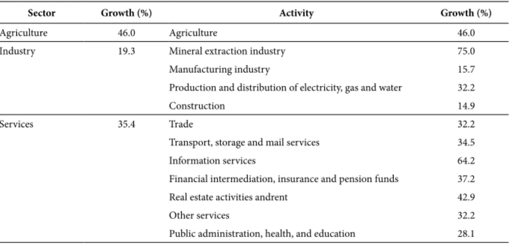
Table 1 shows the percentage output growth between 2000 and 2009, at constant prices, for the 12 activities and their respective aggregations. Note, for instance, that the mineral extraction industry and information services stand out in terms of relative growth (75.0% and 64.2%, respectively).
Table 1 – Output growth between 2000 and 2009
Sector Growth (%) Activity Growth (%)
Agriculture 46.0 Agriculture 46.0
Industry 19.3 Mineral extraction industry 75.0
Manufacturing industry 15.7
Production and distribution of electricity, gas and water 32.2
Construction 14.9
Services 35.4 Trade 32.2
Transport, storage and mail services 34.5
Information services 64.2
Financial intermediation, insurance and pension funds 37.2
Real estate activities andrent 42.9
Other services 32.2
Public administration, health, and education 28.1
Source: Data compiled by the author from Input-Output Matrices for 2000 and from the System of National Accounts for 2009, both published by IBGE.
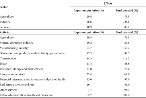
Table 2 summarizes the output growth decomposition as to the effects of input--output relations and of final demand, according to equation (4), but in percentage terms. For example, according to Table 2, 20.5% and 79.5% of the growth of the
cultural sector was due, respectively, to the effects of input-output relations and of final
demand9.
Table 2 – Effects on output growth between 2000 and 2009
Sector
Effects
Input-output ratios (%) Final demand (%)
Agriculture 20.5 79.5
Industry -28.8 128.8
Services 10.9 89.1
Activity Input-output ratios (%) Final demand (%)
Agriculture 20.5 79.5
Mineral extraction industry 19.2 80.8
Manufacturing industry -53.7 153.7
Generation and production of electricity, gas and water 17.5 82.5
Construction -14.3 114.3
Trade 11.4 88.6
Transport, storage and mail services 21.0 79.0
Information services 32.4 67.6
Financial intermediation, insurance andpension funds 13.0 87.0
Real estate activities and rent 16.1 83.9
Other services 1.7 98.3
Public administration, health and education -2.7 102.7
Source: Data compiled by the author based on the Input-Output Matrices for 2000 and the System of National Accounts data for 2009, both published by IBGE.
Three important conclusions can be drawn from Table 2. First, it can be noted that final demand was the major factor of growth for all activities in the 2000s.
Second, input-output relations contributed to the contraction of two industrial activities: manufacturing and construction. In other words, a lower intermediate con-sumption of inputs supplied by these two activities accounted for a decrease in their
output equivalent to 8.4%10 and 2.1%11, respectively. At a more aggregate level, this lower
intermediate consumption led to a decrease of 5.6%12 in industrial output.
9 Therefore, once that, according to Table 1,agriculture had a 46% growth, the effects of input-output rela-tions and of final demand accounted for the respective growths of 9.4% (46% × 20.5%) and 36.5% (46% × 79.5%) of this sector.
Third, the effects of input-output relations and of final demand yielded a growth
of -5.6%13and 24.9%14, respectively, for the industry, and 3.8%15 and 31.6%16 for
servi-ces. Therefore, the growth differential between services and industry induced by the
effects of input-output relations corresponds to 9.4%17 (accounting for 59% of the
16.1% differential), while that induced by the effects of the final demand amounts to
6.7%18 (or 41% of the overall differential).
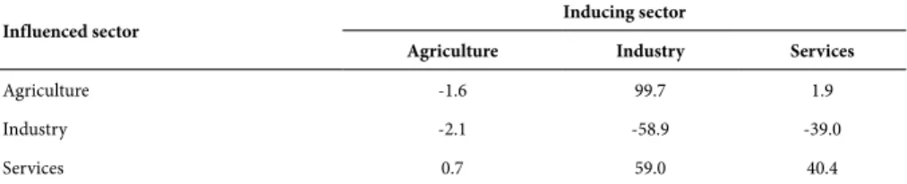
Table 3 shows the sectors responsible for the effects of input-output relations on
each sector19. For example, recall that, according to Table 2, the increase in
interme-diate consumption of agricultural inputs accounted for a 20.5% growth of this sector. Thus, according to Table 3, 99.7% of this growth originated from an increase in inter-mediate consumption was induced by industry, while percentages equivalent to 1.9% and -1.6% were induced, respectively, by the service and agricultural sectors.
Table 3 – Decomposition of the effects of input-output relations (%)
Influenced sector
Inducing sector
Agriculture Industry Services
Agriculture -1.6 99.7 1.9
Industry -2.1 -58.9 -39.0
Services 0.7 59.0 40.4
Source: Data compiled by the author based on the Input-Output Matrices for 2000 and the System of National Accounts data for 2009, both published by IBGE.
Two conclusions can be established from Table 3. First, the smaller demand for industrial inputs, which was responsible for a reduction in industrial output, is a com-mon phenomenon to the production chains of the three sectors. Second, a larger de-mand for inputs necessary to produce industrial goods was relevant to the growth of both the agricultural and the service sectors (but especially for the former one).
13 19.3% (Table 1)
× (-28.8%) (Table 2) = -5.6%.
14 19.3% (Table 1) × 128.8% (Table 2) = 24.9%. 15 35.4% (Table 1) × 10.9% (Table 2) = 3.8%. 16 35.4% (Table 1)
× 89.1% (Table 2) = 31.6%.
17 3.8% - (-5.6%) = 9.4%. 18 31.6% - 24.9% = 6.7%.
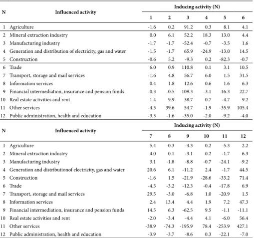
Table 4 exhibits the same results of Table 3, but disaggregated into the 12 activities. Note that the positive effects for agriculture and services from the larger intermediate consumption of inputs supplied by these sectors for the production of industrial goods
were caused mainly by the production chain of the manufacturing industry20.
Table 4 – Disaggregated decomposition of the effects of input-output relations (%)
N Influenced activity
Inducing activity (N)
1 2 3 4 5 6
1 Agriculture -1.6 0.2 91.2 0.3 8.1 4.1
2 Mineral extraction industry 0.0 6.1 52.2 18.3 13.0 4.4
3 Manufacturing industry -1.7 -1.7 -52.4 -0.7 -3.5 1.6
4 Generation and distribution of electricity, gas and water -1.5 -1.7 65.9 -24.9 -13.0 14.5
5 Construction -0.6 5.2 -9.3 0.2 -82.3 -0.7
6 Trade 6.0 0.9 110.8 0.1 3.1 10.5
7 Transport, storage and mail services -1.6 4.8 56.7 6.0 1.5 31.5
8 Information services 0.4 1.8 12.6 0.6 1.6 6.3
9 Financial intermediation, insurance and pension funds -0.3 -0.5 109.3 -3.1 16.3 22.7
10 Real estate activities and rent 1.4 9.9 38.7 0.7 -4.7 9.2
11 Other services -4.5 39.6 54.7 -1.9 -35.9 105.4
12 Public administration, health and education -3.3 -1.6 -35.0 -2.0 -9.2 -4.0
N Influenced activity
Inducing activity (N)
7 8 9 10 11 12
1 Agriculture 5.4 -0.3 -4.3 0.2 -5.3 2.2
2 Mineral extraction industry 4.0 0.1 -3.1 0.2 -1.7 6.3
3 Manufacturing industry 3.1 -1.8 -8.8 -0.7 -24.1 -9.2
4 Generation and distributionof electricity, gas and water 20.6 6.1 -11.2 2.4 -1.7 44.5
5 Construction -1.6 1.5 -21.9 -28.6 -33.2 71.4
6 Trade -4.5 -3.2 -12.3 -0.4 -17.8 6.9
7 Transport, storage and mail services 29.5 -3.0 -6.8 1.0 -20.9 1.5
8 Information services 2.4 13.4 4.4 1.9 7.2 47.3
9 Financial intermediation, insurance and pension funds 14.5 6.3 -62.5 9.5 -1.1 -11.1
10 Real estate activities and rent -2.0 -3.4 -4.4 4.1 -6.0 56.4
11 Other services -38.9 -74.3 -195.9 78.4 -253.9 427.1
12 Public administration, health and education -3.9 -3.7 -8.6 0.3 -22.1 -7.0
Source: Data compiled by the author based on the Input-Output Matrices for 2000 and the System of National Accounts data for 2009, both published by IBGE.
Table 5 allows the identification of the share of growth of each sector induced by the final demand from each of the other sectors. In this way, it can be seen that, on the one hand, the increase in the final demand for industrial goods had a significant impact on
the growth of agriculture (accountable for a 10.8%21 increase in the output of this sector),
and, on the other hand, the increase in the final demand for services was also relevant for
the growth of industry (leading to an increase of 5.1%22 in the industrial output).
Table 5 – Decomposition of the effects of final demand (%)
Influenced sector
Inducing sector
Agriculture Industry Services
Agriculture 60.3 29.4 10.3
Industry 3.3 76.2 20.5
Services 1.0 9.9 89.1
Source: Data compiled by the author based on the Input-Output Matrices for 2000 and the System of National Accounts data for 2009, both published by IBGE.
3.1. FINAL DEMAND COMPONENTS
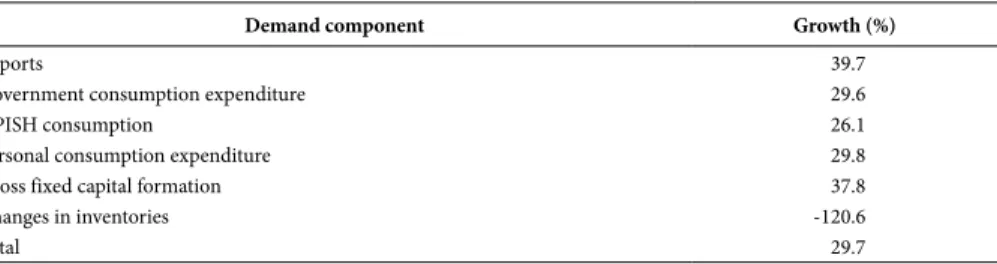
The final demand item of the System of National Accounts consists of the sum of six components: exports, government consumption expenditures, consumption of non-profit institutions serving households (NPISH), personal consumption expenditures, gross fixed capital formation and changes in inventories. Table 6 shows the percentage growth of each one of these components throughout the period between 2000 and 2009.
Table 6 – Growth of the final demand components between 2000 and 2009
Demand component Growth (%)
Exports 39.7
Government consumption expenditure 29.6
NPISH consumption 26.1
Personal consumption expenditure 29.8
Gross fixed capital formation 37.8
Changes in inventories -120.6
Total 29.7
Source: Data compiled by the author based on the Input-Output Matrices for 2000 and the System of National Accounts data for 2009, both published by IBGE.
Table 7 exhibits the percentage values of the effects of final demand on each sector for which the respective components were accountable. For instance, note that, accor-ding to Table 2, the effects of the final demand accounted for 79.5% of the growth of
agriculture. In its turn, Table 7 shows that exports account for 34.9% of these effects. Thus, these exports led alone to a 12.7% growth (46.0% × 79.5% × 34.9%) of the agri-cultural sector between 2000 and 2009.
Table 7 – Decomposition of the effects of final demand, by its components (%)
Sector
Demand component
Exports Government consumption
expenditure NPISH consumption
Agriculture 34.9 3.5 0.3
Industry 18.1 7.5 0.6
Services 9.1 25.5 1.7
Sector
Demand component
Personal consumption expenditure
Gross fixed capital
formation Changes in inventories
Agriculture 50.9 23.1 -12.7
Industry 51.1 36.9 -14.2
Services 57.0 8.7 -2.0
Source: Data compiled by the author based on the Input-Output Matrices for 2000 and the System of National Accounts data for 2009, both published by IBGE.
According to Table 7, both for agriculture and for industry, the most relevant final demand components were exports, personal consumption expenditure and gross fixed capital formation. Conversely, the most relevant components for the service sector appear to have been government and personal consumption. It may therefore be con-cluded that, on the one hand, exports and gross fixed capital formation had significant impacts on the agricultural and industrial sectors, but only secondary effects on servi-ces. On the other hand, the opposite was observed for government consumption: a relevant effect on services, but a secondary one on the other sectors.
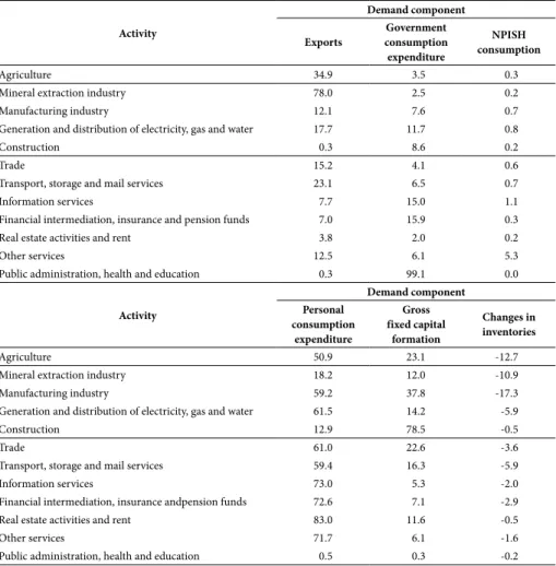
Finally, Table 8 shows similar results to those of the previous table, but disaggrega-ted into the 12 activities that make up the sectors. As to the industrial sector, this de-composition allows a clearer distinction between the effects of each component of fi-nal demand: the mineral extraction industry was fostered mainly by exports; the manufacturing industry, by personal consumption and by gross fixed capital forma-tion; generation and distribution of electricity, by personal consumpforma-tion; and, finally, the construction industry, by gross fixed capital formation.
Table 8 – Disaggregated decomposition of the effects of final demand, by its components (%) Activity Demand component Exports Government consumption expenditure NPISH consumption
Agriculture 34.9 3.5 0.3
Mineral extraction industry 78.0 2.5 0.2
Manufacturing industry 12.1 7.6 0.7
Generation and distribution of electricity, gas and water 17.7 11.7 0.8
Construction 0.3 8.6 0.2
Trade 15.2 4.1 0.6
Transport, storage and mail services 23.1 6.5 0.7
Information services 7.7 15.0 1.1
Financial intermediation, insurance and pension funds 7.0 15.9 0.3
Real estate activities and rent 3.8 2.0 0.2
Other services 12.5 6.1 5.3
Public administration, health and education 0.3 99.1 0.0
Activity Demand component Personal consumption expenditure Gross fixed capital formation Changes in inventories
Agriculture 50.9 23.1 -12.7
Mineral extraction industry 18.2 12.0 -10.9
Manufacturing industry 59.2 37.8 -17.3
Generation and distribution of electricity, gas and water 61.5 14.2 -5.9
Construction 12.9 78.5 -0.5
Trade 61.0 22.6 -3.6
Transport, storage and mail services 59.4 16.3 -5.9
Information services 73.0 5.3 -2.0
Financial intermediation, insurance andpension funds 72.6 7.1 -2.9
Real estate activities and rent 83.0 11.6 -0.5
Other services 71.7 6.1 -1.6
Public administration, health and education 0.5 0.3 -0.2
Source: Data compiled by the author based on the Input-Output Matrices for 2000 and the System of National Accounts data for 2009, both published by IBGE.
4. CONCLUSIONS
In addition, this paper shows that if, on the one hand, the increase in final demand played an important role in the growth of the Brazilian economy in the 2000s, on the other the magnitude and direction of the influence of each component of this demand were quite heterogeneous. In fact, the results allowed drawing the following conclusions:
(i) Personal consumption was relevant for the whole economy.
(ii) Gross fixed capital formation was important to both the manufacturing and construction industries.
(iii) Exports were relevant mainly to the mineral extraction and agricultural in-dustries.
(iv) Government consumption had a significant impact only on public adminis-tration, health and education services, in addition to a secondary but impor-tant effect on information and financial intermediate on services. In the re-mainder of the economy, it played a less important role.
It was not within the scope of the present study to assess whether the concern with the smaller share of industry in the GDP is valid, or whether compensatory measures for the industry are desirable. However, it is possible to conclude that, if policy makers are interested in such compensatory measures and if one wants to offset the changes in the production structure with stimulus for the aggregate demand, one should create incentives for gross fixed capital formation, to the detriment of government consump-tion. This conclusion is supported by Dasgupta and Singh (2006) and Rowthorn and Ramaswamy (1999), who find positive correlations between the level of gross fixed capital formation and the share of manufacturing in employment and production.
However, Dos Santos and Pires (2009) show that private investment in Brazil is little sensitive to changes intaxes, implying that the ability of policymakers to induce an increase in the former variable through the traditional tools of fiscal policyis very limited. In this sense, Demir (2009) employs a model of portfolio choice in order to explain the low investment rates of three developing countries (Argentina, Mexico and Turkey) during the 1990s. The author argues that, given risk, uncertainty, imperfec-tions in capital markets and relative returns, firms may prefer to make reversible short--term financial investments than irreversible longshort--term fixed ones. This can also be the reason lying behind the insensitivity of Brazilian private investment in relation totaxes, but that remains a hypothesis to be investigated in future research.
5. REFERENCES
BONNELLI, R.; PESSÔA, S. A. Desindustrialização no Brasil: um resumo da evidência. Texto para Discussão, IBRE, Fundação Getúlio Vargas, n. 7, 2010.
DASGUPTA, S.; SINGH A. Manufacturing, services and premature deindustrialization in deve-loping countries – a Kaldorian analysis. UNU-WIDER Research Paper, n. 2006/49, 2006. DEMIR, F. Financial liberalization, private investment and portfolio choice: financialization of
real sectors in emerging markets. Journal of Development Economics, v. 88, n. 2, p. 314-324, 2009.
DOS SANTOS, C. H.; PIRES, M. C. C. Qual a sensibilidade dos investimentos privados a au-mentos na carga tributária brasileira? Uma investigação econométrica. Revista de Economia Política, v. 29, n. 3, p. 213-231, 2009.
FELDMAN, S. J.; MCCLAIN, D.; PALMER, K. Sources of structural change in the United States, 1963-78: An input-output perspective. The Review of Economics and Statistics, v. 69, n. 3, p. 503-510, 1987.
GUILHOTO, J.; SESSO FILHO, U. Estimação da matriz insumo-produto utilizando dados pre-liminares das contas nacionais: aplicação e análise de indicadores econômicos para o Brasil em 2005. Revista Economia e Tecnologia, v. 6, n. 4, p. 53-62, 2010.
KONGSAMUT, P.; REBELO, S.; XIE, D. Beyond balanced growth. Review of Economic Studies, v. 68, n. 4, p. 869-882, 2001.
KUZNETS, S. Modern economic growth: rate, structure and spread. New Haven and London: Yale University Press, 1966
LIM, H.; YOO, S.; KWAK, S. Industrial CO2 emissions from energy use in Korea: A structural decomposition analysis. Energy Policy, v. 37, n. 2, p. 686-698, 2009.
MA, C.; STERN, D. I. China’s changing energy intensity trend: A decomposition analysis. Energy Economics, v. 30, n. 3, p. 1.037-1.053, 2008.
MACIENTE, A. N. The determinants of agglomeration in Brazil: input-output, labor and know-ledge externalities. Doctoral dissertation, Agricultural and Consumer Economics, Graduate College, University of Illinois, Urbana-Champaign, 2013.
NASSIF, A. Há evidências de desindustrialização no Brasil? Revista de Economia Política, v. 28, n. 1, p. 72-96, 2008.
NGAI, L. R.; PISSARIDES, C. A. Structural change in a multisector model of growth. American Economic Review, v. 97, n. 1, p. 429-443, 2007.
OREIRO, J. L.; FEIJÓ, C. A. Desindustrialização: conceituação, causas, efeitos e o caso brasileiro.
Revista de Economia Política, v. 30, n.2, p. 219-232, 2010.
ROSE, A.; CASLER, S. Input–output structural decomposition analysis: a critical appraisal. Eco-nomic Systems Research, v. 8, n. 1, p. 33-62, 1996.
ROWTHORN, R.; RAMASWAMY, R. Growth, trade, and deindustrialization. IMF Staff Papers, v. 46, n. 1, p. 18-41, 1999.