Rev. Econ. Contemp., Rio de Janeiro, v. 15, n. 3, p. 483-511, set-dez/2011 483 * Artigo recebido em 21/03/2011 e aprovado em 12/01/2012.
1991-1998
Geraldo Edmundo Silva Junior
**ABSTRACT: his paper presents an empirical contribution to the identiication of
Grossman-Helpman’s “Protection for Sale” parameters model for Brazilian trade policy, based on robust estimations techniques, which means the use of instrumental variables in a 2SLS for Generalized Method of Moments and Limited Information Maximum Likelihood methods for weak instruments with corrections of size tests, in order to correct endogenous bias. he results suggest that the political economy of Brazil’s trade policy is an outlier in international comparisons, as the identiication of structural parameters for Protection for Sale model shows a low part of population represented by an interest group and low weight of the welfare function.
KEYWORDS: political process; rent-seeking; lobbying; elections; legislatures; and
voting behavior; trade policy; international trade organizations; country; industry studies of trade.
JEL Code: D72; F13; F14.
POLÍTICA COMERCIAL ENDÓGENA
BRASILEIRA: 1991-1998
RESUMO: O presente trabalho é uma contribuição empírica para a identiicação dos
parâmetros do modelo “Protection for Sale” de Grossman e Helpman para a política comercial brasileira, baseado em técnicas de estimação robustas, o que signiica o uso de variáveis instrumentais em um procedimento de Mínimos Quadrados em Dois Estágios (MQ2E) para o Método dos Momentos Generalizados (GMM) e o Método de Máxima Verossimilhança com Informação Limitada (FIML) para instru-mentos fracos com correções dos tamanhos dos testes para a correção da tendência de endogamia. Os resultados mostram que a economia política da política comercial
** Doutor em Economia pela Universidade Federal do Rio Grande do Sul e professor do Programa de
brasileira é atípica em relação às comparações internacionais, pois a identiicação dos parâmetros estruturais para o modelo de Proteção de Vendas mostra uma pequena parcela da população representada por um grupo de interesses e uma baixa ponderação da função de bem-estar social.
PALAVRAS-CHAVE: processos políticos; busca de renda; lobbying; eleições;
1. INTRODUCTION
he literature on the Endogenous Trade Policy heory reveals that the research object should not be only the economic system, but also the political inluence of agents and coalition formation in political system. herefore, the inference about optimal results extrapolated the scope of economic analysis. For Nelson (1988), the research agenda imposed the condition, in which, the decision making should be based on the structure of hypothesis on political system and in the interaction amongst gover-nments and private agents, either represented by lobbies or not.
he Endogenous Trade Policy heory has been an important role for economic literature, in response to the liberalization policies support and their endorsement by decision-makers. Also, it is observed tarif line speciication depended on the results of two stage game involving internal that the agents, private agents against a incum-bent govern, a and external agents, represented by discussions amongst trade part-ners or members in an international forum.
he theory would be the result of the intellectual efort, from economists and political scientists, to explain the determination of the domestic protection levels. he endogenous approach has been promoted by the following observations: (i) the awareness of a disparity between the propositions held by economists about free trade and economic authorities’ practices; (ii) the lack of a relation to economic optimum and the political optimum; and, (iii) the existence of a political market where the protection level was negotiated and determined.
he literature of endogenous policy theory was an answer to the non-exogenous aspect in domestic protection’s level. So, in the eighties, it sourced a set of frameworks for endogenous protection to substitute the ad hoc models 70’s, namely:
a) Hillman (1982), Cassing, Hillman and van Long (1985), Hillman and Ursprung (1988), van Long and Vousden (1991), Brainard and Verdier (1994), Laphan and Ware (2001) and Hillman, van Long and Soubeyran (2001) derived a political support function that edged the policymakers trade actions constraints that causes welfare reduction;
b) Tarif formation function derived from Findlay and Wellisz (1983), Feenstra and Bhagwati (1983), Rodrik (1986), and Wellisz and Wilson (1986) that established a linear relationship amongst contributions from lobbies and tarifs;
c) Median elector model derived for Mayer (1984) suggested that the median elector chooses the level of protection;
e) Grossman and Helpman (1994) derived the political contributions model, a parsimoniously framework from game theory in a irst price menu auction under complete information, in which interest groups and incumbent government interaction results in a level of protection. Trade wars and trade talk’s model, in Grossman and Helpman (1995a), and free trade area, in Grossman and Helpman (1995b), sourced from PS Model.
So, for a small country, Grossman and Helpman (1994) established a single model, to determine endogenous trade protection through and parsimonious contri-butions by organized and prominent sectors, named Protection for Sale model, PS model hereater.
he framework is based on a two stage game amongst an incumbent govern-ment and industrial sectors. he objective of incumbent governgovern-ment is maximize the govern function, which weighted political contributions from organized sectors and aggregated well-being. hrough contributions, the sectors accessed the political deci-sions on tarifs barriers. Empirical literature suggested the opposite relation between parts of government function. So, with the both parameters, namely, a weight of well--being function and proportion of organized population in interest groups deter-mined the sectors protection levels.
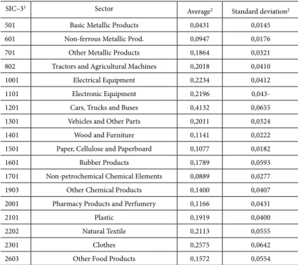
Table 1 – Basic statistics of sectorial tarifs
SIC–31 Sector
Average2 Standard deviation2
501 Basic Metallic Products 0,0431 0,0145
601 Non-ferrous Metallic Prod. 0,0947 0,0176
701 Other Metallic Products 0,1864 0,0321
802 Tractors and Agricultural Machines 0,2018 0,0410
1001 Electrical Equipment 0,2234 0,0412
1101 Electronic Equipment 0,2196
0,043-1201 Cars, Trucks and Buses 0,4132 0,0655
1301 Vehicles and Other Parts 0,2011 0,0324
1401 Wood and Furniture 0,1141 0,0222
1501 Paper, Cellulose and Paperboard 0,1077 0,0182
1601 Rubber Products 0,1789 0,0593
1701 Non-petrochemical Chemical Elements 0,0889 0,0277
1903 Other Chemical Products 0,1400 0,0407
2001 Pharmacy Products and Perfumery 0,1166 0,0431
2101 Plastic 0,1919 0,0400
2202 Natural Textile 0,2113 0,0555
2301 Clothes 0,2575 0,0642
2603 Other Food Products 0,1572 0,0554
Notes: (1)Standard Industrial Code (three digits),(2)Parameters referring to the period of 1991-1998.
Source: Results achieved and organized by the author.
With the basic statistics of the ad valorem tarifs, summarized in Table 1, it was observed that the average of the sector tarifs, like: Basic Metallic Products and Non--Ferrous Metallic Products, would be considered as low. Sectors as Automobiles, Trucks and Buses, Clothes, Natural Textiles, Electrical Equipment and Electronic Equipment would be considered as high. By taking the standard deviation, since the period of 1991-1998 includes the launching process of the MERCOSUR Agreement, and the beginning of the deterioration of the commercial relations amongst members as of 1997, because of the Asian crisis, it was observed that sectors as Automobiles, Trucks and Buses, Rubber Products, Natural Textiles, Clothes and Other Food Products presented a high standard deviation in comparison to the other sectors.
Considering the references of Calfat, Ganame, and Flores (2001) and Facchini et al. (2010) that implied partial identiication of PS Model for Argentina, Brazil, Para-guay, and UruPara-guay, by the irst and for Latin America and South Cone, the second one, is suggested that Brazilian trade policy had been established endogenously.
So, the hypothesis of the present paper is to verify if the model was suitable or not for the Brazilian economy in the period of 1991-1998, although the inluence of trade agreement amongst Argentina, Brazil, Paraguay and Uruguay.
his paper uses panel data methodology that refers to multidimensional data to reveal the Brazilian data support to PS model framework. he dimensional perspective is shown by eighteen industrial sectors, by cross-section dimension, and eight years (1991 to 1998), by time series dimension. We added Armington’s elasticity1, which
is time invariant. For the indicator estimation for interest group organization, we use random efects Tobit regression censored. In response to endogenous bias, presented in endogenous protection models, we use weak instruments in 2SLS for the Genera-lized Method of Moments (GMM) and Limited Information Maximum Likelihood (LIML) procedures, with correction of size tests.
2. EMPIRICAL RESULTS WITH ENDOGENOUS TRADE POLICY MODELS2
Besides some theoretical empirical contributions in literature of Endogenous Trade Policy, only ater PS model, suggested by Grossman and Helpman (1994), a new theo-retical line of propositions, with rigorous empirical tests, corroborates endogenous trade policies endogenous properties.
he contributions outitted by Grossman and Helpman’ paper (1994) considered the following modiications: the greater number of agents involved in the deal, the formulation of agreements of free trade with and without symmetry, and the parti-cipation of foreign lobbies in the domestic scenery3. It must be included the
endoge-nous aspect of lobbies, proposed by Mitra (1999).
he pioneering characteristic of the empirical treatment, related to the PS model, was due to Goldberg and Maggi (1999) seminal paper. hose authors observed that the predictions of the PS model were consistent with the data of the North-American economy in 1983, identifying the structural model parameters in their original formulation.
Besides, they tested whether the inclusion of other variables, which were impor-tant in ad-hoc models, afects the model explanatory power. Such variables are
rele-1 The use of the Armington’s elasticity for the PS model test was initially proposed by Gallaway,
McDaniel, and Rivera (2003).
2 Gawande and Krishna (2005) reviewed some empirical papers on endogenous protection, until 2001,
without incorporating the results of Eicher and Osang (2002), Calfat, Flôres, and Ganame (2000), and posterior publications.
vant to the equations of tarif and non-tarif barriers (employment rate, sectorial unemployment rate, unionization, changes in the import penetration and concentra-tion of buyers and sellers, among others).
he speciication was also tested for Argentina, Brazil, Paraguay, and Uruguay by Calfat, Flores and Ganame (2000). hose authors concluded that the model also would be applicable to the MERCOSUR case, since the partial results allowed the identiication of the correct signs for Brazil and Uruguay. It was also identiied, in 1996, the proportion of the voting population that should be represented by an inte-rest group in Brazil and Uruguay, with parameter values of 0.67 and 0.86, respectively, without the identiication of the weighted parameter.
he empirical strategy suggested by authors evolved a hree-Stages Leas Squares (3SLS) that combines 2SLS with Seemingly Unrelated Regression (SUR). he problem with procedure was that authors take the SUR stage equivalent to Ordinary Least Square (OLS).
he heteroscedasticity were used in the same procedure as Goldberg and Maggi (1999). In the same way, although with the aim of measuring Latin America’s reaction about the increase in imports from China and India, Facchini et al. (2010) identiied the aggregated weight well-being function to Latin America (a = 918), and South Cone (a = 1639). hose authors used China and India’s participation in product’s world trade and US capital-labor as instrumental variables. hey do not presented any test to the quality of instruments or the correction of sample size.
Considering the partial results and procedure limitations for Calfat, Flores and Ganame (2000) and, also, the aggregation for Latin America and limitations of empi-rical procedure to Facchini et al. (2010), our paper presents the identiication of all Brazilian PS model parameters based on robust procedure.
he Eicher and Osang (2002) test, applied to the American economy in 1983, proved that the PS model were superior to the Tarif Formation Function model, by Feenstra and Bhagwati (1983).
Conventional use of the original equation also produced favorable results for Turkey. Mitra, homakos and Ulubasoglu (2002) applied the model in periods from 1983 to 1990, which resulted in a higher weight of the welfare function in democratic period, and changes in the speciication of the original model allowed the inclusion of theoretical relevant variables. Gawande and Bandyopadhyay’s paper (2000), and McCalman’s paper (2004) enrolled the list of empirical papers for PS model.
On the other hand, McCalman’s paper (2004), applied to Australia using the same method, demonstrated that, with data to the periods from 1968 to 1969, and from 1991 to 1992, the percentage of the voting population organized in an interest group increased due to the commercial liberalization, which took place in the second period. here was no statistically signiicant diference for the weight of welfare func-tion in both periods. Bohara, Gawande, and Sanguinetti (2004) pursued to empiri-cally identify the Argentinean and Brazilian sectors presented in the list of exceptions to the Common External Tarif (CET). hey adapted Grossman and Helpman’s model (1995a, 1995b), an extension of the PS model. With information regarding to tarifs and non-tarif barriers, during period from the irst quarter of 1992 to the fourth quarter of 1994, they concluded that the model was not able to explain the reason for the exclusion of some CET sectors.
Finally, modiication presented by Gawande, Krishna, and Robbins (2006), applied to the data concerning USA economy, in periods of 1978-1979 and 1981-1982, was speciied to include the foreign lobbies in the protection equation of the PS model. he objective was to verify the inluence of foreign interest groups in the determination of the American protection structure.
Results reveal that PS model, modiied for the inclusion of external lobbies, was strong and statistically signiicant. In other words, the signs of the estimated parame-ters were not altered with the inclusion of other variables.
he diferences proposed for the empirical treatment in the present paper are the use of the Armington’s elasticity, as proxy of the price elasticities in demands for imports; the speciication of instrumental variables compatible with sectorial struc-tures and conjuncstruc-tures; the use of panel data techniques for a period of eight years, aiming at the capture of the inter- and intra-sectorial dynamic efects in the time interval studied and, since PS model structure is a balance result, statistical signii-cance reveals consistency; and, inally, the use of tarif aliquots, which would origi-nally be represented in the PS model.
instruments to control the bias of endogenous aspect. Finally, we managed the problems of heteroscedasticity and autocorrelation.
3. METHODOLOGY
he methodology was based on the use of panel data techniques with the speciica-tion of instrumental variables, for the eliminaspeciica-tion of the endogenous bias presented in such models, as proposed by Treler (1993). Estimates were applied for the data concerning Brazilian economy, in period from 1991 to 1998, comprising the commer-cial openness, started in 1991, the admission of the country in the MERCOSUR in 1995, and the beginning of its collapse in the end of 1998.
3.1 THE EMPIRICAL MODEL TESTED
he basic model developed by Grossman and Helpman (1994) considers an objective function of an incumbent government given by:
h L h
( )
( )
G C p aW p
∈
=
∑
+ (1)in which:
C = campaign contributions;
L = sectors organized in interest groups;
h = h–th activity sector;
a = weight of the welfare function;
W = welfare function; p = price vector.
he government objective-function demonstrated to be additive to the resources from contributions of interest groups and some weight of the welfare function.
he public welfare function W(p) would represent the sum of these functions to the results of each of the i–th sectors of the economic activity, according to the identity (2):
( )
1( )
n i i
W p =
∑
=W p (2)in which:
he structure of protection is derived from a menu-auction problem, or a two-stage game, in which sectors contributions through lobbies are limited to a feasible set. Based on contributions, government established the optimal trade policy with maximization of his objective function. As this game is repeated, the strategic contributions forced government to best choices to lobbies as a Truthful Nash Equilibria, as equation (3) described:
( )
( )
( )
( )
0 0 0 0 0 0 0 0,
j j i L i
W p C p C p a W p j L
∈
∇ − ∇ +
∑
∇ + ∇ = ∀ ∈ (3)Solving the problem for (3), based on equations (1) and (2), generates equation (4).
(
) ( )
(
*) ( ) (
' *) ( )
' 0j L j j L j j j j j j j j
I −α y p +α p −p m p +a p p m− p = (4)
By rearranging equation (4), and solving it for τi = (pi – pi*)/pi*, result the expres-sion (5), plus an index for speciication to time:
1
it it L it
it
L it
I z
y
it e
τ α
τ α α
−
= =
+ + (5)
in which:
y = tarif relation;
τ = ad valorem import tarif;
z = inverse import penetration;
I = interest group representation indicator;
e = price–elasticity of the demand for imports;
i = activity sector, i = 1, ...., n; and
t = time unit, t = 1991, ...., 1998.
3.2 ECONOMETRIC MODEL: THE PANEL DATA METHOD
collinearity among variables, and the possibility of interaction between cross-sections and time units of those sets, signiicant to the study of dynamic adjustment.
he inferences on the model results would be done based on the estimations of equations (6) and (7), written with the price elasticity of demand for imports in irst member, Model 1, or with the price elasticity of demand for imports in second member, Model 2, namely:
1
it
it i i it it it it
it
y e τ e yz δz υ µ τ
= = + + +
+ (6)
in which:
0
it
L Î a γ
α =
+ ;
L
L a
α δ
α =
+ ;
L δ α
γ = −
1
a δ
γ + =
z = inverse import penetration;
υ = random residuals to measure random efects;
m = deterministic residuals to measure ixed efects.
1
it it it
it i it i
it i i
z z
y e u
e e
τ γ δ υ
τ
= = + + +
+ (7)
Some problems appear in estimation process for PS model. So, an empirical stra-tegy must nullify them.
3.3 DATA TREATMENT AND EMPIRICAL STRATEGY
In the veriication of the endogenous aspect of the Brazilian trade policy, two econo-metric diiculties were found. he irst econoecono-metric diiculty was the speciication of the dummy variable to the organization in industrial sectors.
he empirical literature presented some alternatives to estimate the organization’s indicator in interest group. Goldberg and Maggi (1999) tried a double censored Tobit model using non-trade barriers. hat proposal was followed by other authors, such as Gawande and Bandyopadhyay (2000), Mitra, homakos and Ulubasoglu (2002), Eicher and Osang (2002), McCalman (2004), and Gawande, Krishna, and Robbins (2006).
Beloc and Guerrieri (2008) used an arbitrary level of 70% to characterize an orga-nized sector in a probit model. Likewise Hagemejer and Michalek (2008) used the sample mean to identify an organized sector, but without an estimation process. A discriminant analysis was used by Mitra, homakos and Ulubasoglu (2002) and Mitra, homakos and Ulubasoglu (2006).
In the present work, sectors that presented a concentration index, for hypothesis, are protected by an import tarif superior to 10%4. So, a Tobit model for a censored
variable was estimated.
0
it it i
I =wβ ϕ+ (8)
in which:
0
it
I = interest group indicator;
wit = vector of independent variables;
β = vector of coeicients; and
ϕi = random efect.
he set of independent variables corresponds to inverse import penetration (zit) industrial concentration index (iciit), number of irms (ne500it), employment turnover rate (treit), export annual coeicients (caeit), annual coeicients of net openness(caalit) and annual coeicients of imported input participation (capiiit), real wage per worker (wit) sectorial employment (lit), increase in sales(cvit), general liqui-dity (lgit), industrial physical production index (ipiit), and imports (mit), all of them presented in the Appendix.
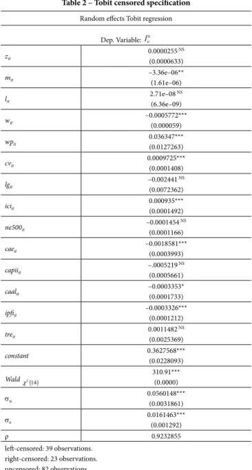
For intervals to the estimation of censored Tobit model5, we have: let side
corres-ponding to non-organized sectors, inferior to “a” level, and right side, the organized sectors, corresponding to level superior to “b”. he estimation results are showed on Table 2.
4 Basic statistics to 18 sectors, from 1991-1998, shows the mean of 14.51%, and standard-deviation of
6.72% in tarifs. he minimum ad valorem tarif was 2.2% and maximum was 37.6%. So, the choice of 10% corresponds to two units of standard-deviation in an asymmetric distribution frequency.
5 he speciication requires the joint density of censored Tobit Model, the observed data in panel data,
Table 2 – Tobit censored speciication
Random efects Tobit regression
Dep. Variable: 0
it
Î
zit
0.0000255 NS (0.0000633)
mit
–3.36e–06** (1.61e–06)
lit
2.71e–08 NS (6.36e–09)
wit
–0.0005772*** (0.000059)
wpit
0.036347*** (0.0127263)
cvit
0.0009725*** (0.0001408)
lgit
–0.002441 NS (0.0072362)
iciit
0.000935*** (0.0001492)
ne500it
–0.0001454 NS (0.0001166)
caeit
–0.0018581*** (0.0003993)
capiiit
–.0005219 NS (0.0005661)
caalit
–0.0003353* (0.0001733)
ipiit
–0.0003326*** (0.0001212)
treit
0.0011482 NS (0.0025369)
constant 0.3627568***
(0.0228093)
Wald 2( )
14
χ
310.91*** (0.0000)
σu
0.0560148*** (0.0031861)
σe
0.0161463*** (0.001292)
ρ 0.9232855
let-censored: 39 observations. right-censored: 23 observations. uncensored: 82 observations.
Notes: (*)10% of significance; (**)5% of significance; (***)1% of significance;
he second problem was the endogenous bias presented in endogenous protec-tion models, deined as the inverse import penetraprotec-tion as an explanatory variable, as well as the price import elasticity.
From empirical literature, diferences amongst alternatives were identiied in the estimation process with Maximum Likelihood for Goldberg and Maggi (1999), and Hagemejer and Michalek (2008); Two Stage Least Square for Gawande and Bandyo-padhyay (2000), McCalman (2004), and Belloc and Gerrieri (2008); Minimum Distance Estimator for Eicher and Osang (2002); Non-Linear Two Stage Least Square Estimation for Mitra, homakos and Ulubasoglu (2002), and Gawande, Krishna, and Robbins (2006); Non-Linear Tobit Limited Information Maximum Likelihood for Gawande and Li (2009).
he strategy to treat price import elasticity endogenous was solved using the elasticity variable in the let-hand side of equation. Strategy was proposed by Goldberg and Maggi (1999), and followed by Eicher and Osang (2002), and McCalman (2004). Diferently, this paper considered the both structures with elasticity in the let-hand side, as equation (6), and in the right-hand side, as equation (7).
Besides the elasticity measurement error problem, due to empirical data set that corresponds to a single year, in the case of Goldbeg and Maggi (1999) and Eicher and Osang (2002), this paper used a larger dataset in which elasticity measurement errors should be less intensive compared to a single year. Moreover, Armington’s elasticities, time invariant, can do better that price import elasticities.
Likewise when you used the price import elasticities in the let-hand side of equa-tion or in the right-hand side, endogenous bias should appear either with tarif efects on domestic production, as a small open country model, or with tarif efects on imports, and consequently on inverse import penetration.
A generalized solution is based on instrumental variables referring to an esti-mation technique used to a variety of violations including measurement error, simultaneity, and omitted variables. Two-Stages Least Squares (2SLS) is gene-rally used as a standard technique. Exception is attributed to Mitra, homakos and Ulubasoglu (2004) that used Weighted Two-Stages Least Square (W2SLS) to manage the endogenous aspect, measurement error problem, and heteroscedas-ticity problem.
Generally, the advantage of 2SLS is an instrumental variable estimation technique that is formally equivalent in linear case, referring this paper. Although, even in an applied instrumental variables procedures to eliminated endogenous bias, another problem appears in instruments’ quality, namely, weak instruments.
In the estimation procedures, we used the Generalized Method of Moments (GMM)6 that allows the achievement of estimated parameters, when the maximum
likelihood requires the non-linear optimization, which is observed in procedures with instrumental variables. he procedure covers the proposal of Mitra, homakos, and Ulubasoglu (2002), and Gawande, Krishna and Robbins (2006). To corroborate the results with this procedure, tests were necessary, since weak instruments cause bias, according to Baltagi (2003).
Classical and robust standard errors are obtained for arbitrary heteroscedasticity to 2SLS instrumental variables procedure in GMM estimation. For Arellano (2002), Sargan’s test is a test of the validity for instrumental variables, basically over identii-cation restrictions.
Using weak instruments in procedure, we need Sargan’s test for Generalized Method of Moments (GMM). So, using instrumental variables is necessary to test the hypothesis requiring correct size when instruments are weak as well as strong7.
Now, the Limited Information Maximum Likelihood procedures (LIML) present advantages in comparison to the other methods, mainly when the number of instru-ments varies in relation to the sample size. Besides, the results of the Monte Carlo simulation showed that the LIML method presents consistent results, even when the instruments are weak, which happened in the analysis, according to Baltagi (2003).
Using weak instruments in LIML procedure requires Anderson-Rubin test (AR), as a test of structural parameters. Also, Lagrange multiplier test (LM) called score test. Recently, Moreira (2003) proposed the Conditional Likelihood Ratio (CLR) test, evaluating tests in the presence of weak instruments8.
For identiication of instruments, according to Greene (1997), it was necessary to adjust the choice of the instruments and the procedure that comprises the following:
• Estimation of the original equation and residuals capture;
• Estimation of a regression between residuals and several potential instru
-ments, including a constant, a trend variable, the lagged dependent varia-bles and the lagged explanatory variavaria-bles. he non-signiicant parameters
6 To GMM procedure with weak instruments, see Baum, Schafer, and Stillman (2003). 7 See Moreira (2003).
were potential instruments, because they did not present correlation with residuals;
• Estimation of the explanatory variables according to the instruments,
where the signiicant parameters were potential instruments, provided that they had not been signiicant in the previous procedure.
In the procedure, the weak and strong instruments used in the two-stage proce-dure were selected. he weak instruments were the non-signiicant ones for equation of the residuals and weakly correlated with endogenous explanatory variables, while the strong or consistent instruments were the non-signiicant for residues and corre-lated with the endogenous explanatory variable.
Finally, to verify the procedure consistency, the regression residues were regressed in two stages, according to the instruments; the non-signiicance of the parameters proved that the residues are consistent.
he advantages of this paper over general literature are (i) it manages the price import elasticity using the both speciication for Model 1 and Model 2; (ii) it consi-dered the Armington’s import elasticity that is time invariant; (iii) the quality of instruments were checked out with a rigorous procedure that determines weak and strong instruments that not appears in other related papers; (iv) even using weak or strong instruments, the Sargan’s test to overidentiication of restrictions was executed; (v) the used alternative of GMM and FIML, the irst based in the non--linear optimization estimation process attributable to the use of instrumental varia-bles, the last based on the variable number of instruments; (vi) the Anderson-Rubin test, Lagrange multiplier test, and conditional likelihood ratio test in the presence of weak instruments in the use of LIML procedure; (vii) the procedure were robust to autocorrelation, heteroscedasticity, or both.
Speciically for Brazilian estimation or aggregated results for Latin America, this paper presented all advantages summarized above.
4. RESULTS AND DISCUSSION
he procedures to reach PS model parameters, as presented in previous section, were based on the estimation of original equation, corresponding to the equations speci-ied as equation (6), as Model 1, and equation (7), as Model 2.
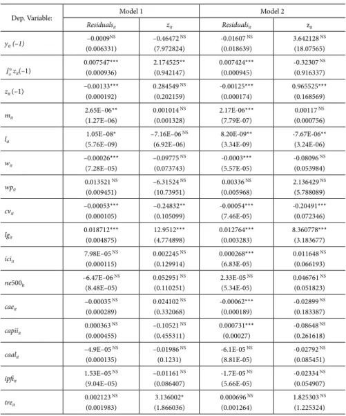
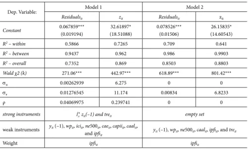
hen, in second step, as implied in Table 3, the residuals estimated were, then, regressed according to the instruments presented in groups of section 3.3, with addi-tion of the lagged dependent variable, and the lagged of endogenous variables, as suggested by Greene (1997). hen, the endogenous variable is regressed (only the inverse of import penetration) according to the variables of the previous regression, as showed on Table 3.
Table 3 – Instruments identiication – maximum likelihood method
Dep. Variable: Model 1 Model 2
Residualsit zit Residualsit zit
yit (–1)
–0.0009NS (0.006331)
–0.46472 NS (7.972824)
-0.01607 NS (0.018639)
3.642128 NS (18.07565)
0
it Î zit(–1)
0.007547*** (0.000936) 2.174525** (0.942147) 0.007424*** (0.000945)
-0.32307 NS (0.916337)
zit (–1)
–0.00133*** (0.000192)
0.284549 NS (0.202159) -0.00125*** (0.000174) 0.965525*** (0.168569) mit 2.65E–06** (1.27E–06)
0.001014 NS (0.001328)
2.17E-06*** (7.79E-07)
0.00117 NS (0.000756)
lit
1.05E–08* (5.76E–09)
–7.16E–06 NS (6.92E–06) 8.20E-09** (3.34E-09) -7.67E-06** (3.24E-06) wit –0.00026*** (7.28E–05)
–0.09775 NS (0.073743)
-0.0003*** (5.57E-05)
-0.08096 NS (0.053984)
wpit
0.013521 NS (0.009451)
–6.31524 NS (10.73951)
0.00336 NS (0.005968)
2.136429 NS (5.788089) cvit –0.00053*** (0.000105) –0.24832** (0.105099) -0.00054*** (7.46E-05) -0.20491*** (0.072346) lgit 0.018712*** (0.004875) 12.9512*** (4.774898) 0.012764*** (0.003283) 8.360778*** (3.183677) iciit
7.98E–05 NS (0.000115)
0.002245 NS (0.129914)
0.000268*** (6.83E-05)
0.011648 NS (0.066193)
ne500it
–6.47E–06 NS (8.48E–05)
0.052951 NS (0.110251)
2.33E-05 NS (5.34E-05)
0.046761 NS (0.051823)
caeit
–0.00035 NS (0.000289)
0.024102 NS (0.332068)
-0.00062*** (0.000189)
-0.02899 NS (0.183387)
capiiit
0.000363 NS (0.000455)
–0.10521 NS (0.455311)
0.000731*** (0.00027)
-0.08648 NS (0.261618)
caalit
–4.9E–05 NS (0.000135)
–0.01986 NS (0.1231)
-6.1E-05 NS (8.81E-05)
-0.02792 NS (0.085451)
ipiit
1.53E–05 NS (9.04E–05)
–0.01161 NS (0.086407)
-1.7E-05 NS (5.66E-05)
-0.02334 NS (0.054907)
treit
0.002123 NS (0.001983)
3.136002* (1.866036)
0.000696 NS (0.001264)
Table 3 – Instruments identiication – maximum likelihood method
Dep. Variable: Model 1 Model 2
Residualsit zit Residualsit zit
Constant 0.067859***
(0.019194)
32.61897* (18.51088)
0.078526*** (0.01506)
26.15835* (14.60543)
R2 – within 0.5866 0.7265 0.709 0.641
R2 – between 0.9437 0.962 0.986 0.9903
R2 – overall 0.7352 0.869 0.8503 0.8803
Wald χ2 (k) 271.06*** 442.97*** 618.89*** 801.42***
σu 0.00262939 6.275 0 0
σe 0.01276545 11.174 0.00834 6.8233
ρ 0.04069975 0.239741 0 0
strong instruments 0
it
Î zit(–1) and treit empty set
weak instruments yit(–1), wpit, iciit, ne500it, caeit, capiiit, caalit,
and ipiit
yit (–1), wpit, ne500it, caalit, ipiit, and treit
Weight ipiit ipiit
Notes: (*)10% of significance; (**)5% of significance; (***)1% of significance; (NS)non-significant; ( ) = standard errors.
hrough the observation of the parameter signiicance, the following initial results were found: (a) Model 1: weak instruments9 (y
it(–1), wpit, iciit, ne500it, caeit,
capiiit, caalit, and ipiit) and strong instruments10 (zit(–1) and treit); and (b) Model 2: weak instruments (yit(–1), wpit, ne500it, caalit, ipiit,, and treit) and no strong instru-ments. To these instruments, an intercept variable and a trend variable, which refers to the years from 1991 to 1998, may be added.
hen, the results for Model 1 and Model 2, using the GMM and LIML methods, were summarized in Table 4 (GMM) and Table 5 (LIML).
9 It can be seen that the variables considered weak instruments were those which simultaneously presented
no correlation with the residuals and weak correlation with the endogenous explanatory variables.
10 he consistent instruments presented non-signiicance in the residuals regression and were statistically
Table 4 – Results of the endogenous protection for the GMM method
Model 1:
1 it
it i i it it it i
it
y e τ e γz δz υ µ τ
= = + + +
+
Model 2:
1
it it it
it i i it i
it i i
z z
y e e u
e e
τ γ δ υ
τ = = + + + + 0 it it it L Î z z a γ α = + 0.10749** (0.0445) 0
it it it it L it
z Î z
e a e
γ α = + 0.0186142*** (0.0094404) L it it L z z a α δ α = + –0.02279** (0.009163) 0
it it it it L it
z Î z
e a e
δ α = + –0.0040473*** (0.0020437) Constant 0.2954094*** (0.0557) Constant 0.15078*** (0.01684) Instrument Variables year, 0 it
Î zit(–1), treit, yit(–1), wpit, iciit, ne500it, caeit, capiiit,
caalit, and ipiit
Instrument Variables wpit, ne500it, caalit, ipiit, andtreit
Instrumented Variables 0
it
Î zitandzit Instrumented Variables Îit0zit and zit
n. observations 144 n. observations 144
F(2, 141) 3.09** F(2, 141) 1.93NS
SQ Residuals 11.674 SQ Residuals 0.30332
SQ Centered Residuals 9.4585 SQ Centered Residuals 0.336724
R2 Centered –0.2343 R2 Centered 0.0992
Sargan’s Statistics 2 9
χ 26.594*** Sargan’s Statistics 2
3
χ 13.252***
Standard errors robust in the presence of arbitrary heteroscedasticity.
Standard errors robust in the presence of arbitrary heteroscedasticity.
Notes: (*)10% of significance; (**)5% of significance; (***)1% of significance; (NS)non-significant. The statistics are
consistent with autocorrelation. The GMM method involved the correction of the heteroscedasticity for the weight
alternative that took into account the square root of the variance of ipfi variable.
Source: Results achieved by the author using Stata Program.
In the basic results corresponding to Table 4, GMM method indicates the signiicant representation to Model 1. Exceptions could be ascribed to the signal of the centered R2. However, Stata procedures show that their negative values did not hinder the
infe-rences about the regression parameters (Sribney, Wiggins, and Drukker, 2003)11.
Sargan’s statistics (Wooldridge, 2002, p. 123; Baum, Schafer, and Stillman, 2003, p. 17), evidenced the overidentiication of the instruments, specifying that, under the null hypothesis, the set of instruments excluded would be valid, besides the non--correlation with residuals for strong instruments. According to the test, the set of instruments are valid, even the correct size is required when they are weak or strong. he Model 2 F-test rejects the structure based on original purpose with the elasticity on second equation member.
Structural parameters estimated, through the signiicance of gamma and delta parameters, which correspond to both variables (inverse import penetration and inverse import penetration by the organization of an interest group), result in the part of population represented by an interest group, aL= 0.21, and the weight of the welfare function, a = 9.09.
Table 5 – Results of the endogenous protection for the LIML method
Model 1:
1 it
it i i it it it i
it
y e τ e γz δz υ µ τ
= = + + +
+
Model 2:
1
it it it
it i i it i
it i i
z z
y e e u
e e
τ γ δ υ
τ = = + + + + 0 it it it L Î z z a γ α = + 0.656234** (0.327027) 0 it it it L Î z z a γ α = + 0.0980684*** (0.0269773) L it it L z z a α δ α = + –0.12993**
(0.064973) it L it
L z z a α δ α = + -0.0190798*** (0.0051416) Constant 0.73344** (0.29961) Constant 0.2216979*** (0.0304048) Instrumental Variables 0 it
Î zit(–1), treit, yit (–1), wpit, iciit, ne500it, caeit, capiiit,
caalit, zit, and ipiit
Instrumental Variables
treit, yit(–1), ne500it, caalit,
0
it
Î zit, and ipiit
Instrumented Variables
zit Instrumented
Variables
zit
n. observations 126 n. observations 126
F(2, 123) 1.98NS F(2, 123) 6.88***
SQ Residuals 84.915 SQ Residuals 1.72536
SQ Cent. Residuals 7.7842 SQ Cent. Residuals 0.242238
R2 Centered –9.9087 R2 Centered –6.1226
H0:_b[zit] –0.33392 H0:_b[zit] –0.018963
Anderson-Rubin = χ92 empty*** Anderson-Rubin =
2 5
χ [–0.037, –0.012679]***
Score (LM)
(–∞,–0.133] U U [0.00098, 0.001] U
U [0.6338, ∞)***
Score (LM) [–0.03712, –0.01266] U
U [0.000302, 0.000346]***
Conditional LR (–∞,–0.133] U
U [0.64, ∞)*** Conditional LR [–0.030206,–0.01377]***
k = 1.22152; λ = 1.24784 e Fuller (#) = 3 k = 1.09094; λ = 1.09941 and Fuller (#) = 1
Note: (*)10% of significance; (**)5% of significance; (***)1% of significance; (NS)non-significant. The statistics are consistent with autocorrelation.
he basic results corresponding to Table 5, now for LIML method, result in the signiicance for Model 2, and no signiicance for Model 1. On the LIML method, results were more robust, since the procedure allows the inclusion of weak instru-ments, without causing bias in the estimated parameters (Cruz and Moreira, 2005). he basic statistics for the use of weak instruments is given by Anderson-Rubin test, Lagrange multiplier (LM) – score test, and conditional probability of CLR statistical that provides the correct sizes for parameters.
he Anderson-Rubin test, a chi-squared test with 5 degrees of freedom, with statistics consistent with autocorrelation produces an instrumented variable coei-cient equal to –0.018963. For LM or score test, the results conirm the parameter for the inverse import penetration relation.
Finally, the conditional probability of CLR statistical, for a = 0.1, results in a signi-icant parameter for delta equal to –0.018963. Combining results for both structural parameters, we achieved part of population represented by an interest group, aL= 0.19, and the weight of the welfare function, a = 10.
In synthesis, the estimations procedures result in adequacy of Model 1 for Brazi-lian economy estimated by GMM method, and Model 2 by LIML method. It provides the adequacy of the model to the Brazilian economy data for the period of 1991-1998, since the parameters αL (referring to the part of the voting population repre-sented by an interest group), and the parameter a (which indicates the weight that the government attributes to the welfare function) corroborated for the endogenous protection hypotheses suggested by Calfat, Flores and Ganame (2000), related to the presence of interest groups in the formulation of the Brazilian trade policy.
5. CONCLUSIONS
he extent of empirical results linked to the proposal of endogenous protection in the trade policy was motivated in the beginning of the 90’s by the series of struc-tured works with the use of the Game heory by Grossman and Helpman (1994). As a result, the contributions of those authors became an important paradigmatic mark of the international economy literature, as well as the empirical results achieved from the econometric works based on their parsimonious structure.
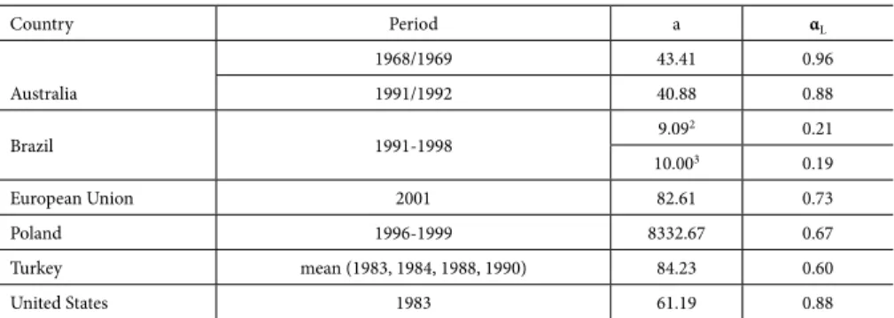
model adequacy based in the identiication of structural parameters for Protection for Sale Model.
Table 6 – Comparative results with the empirical literature
Country Period a αL
Australia
1968/1969 43.41 0.96
1991/1992 40.88 0.88
Brazil 1991-1998 9.09
2 0.21
10.003 0.19
European Union 2001 82.61 0.73
Poland 1996-1999 8332.67 0.67
Turkey mean (1983, 1984, 1988, 1990) 84.23 0.60
United States 1983 61.19 0.88
Source: McCalman (2004); GMM-Model 1;LIML-Model 2; Belloc and Gerrieri (2008); Hagemejer and Michalek (2008);
Mitra, Thomakos, and Ulubasoglu. (2002); Goldberg and Maggi (1999).
Once Brazilian trade policy supported results to PS model, a benchmark, based on results for Australia, European Union, Poland, Turkey, and United States, give us support to international comparisons for new results from empirical literature.
For international comparisons to the results of empirical literature – see Table 6, the parameters, besides the signiicance of structural parameters – Brazilian economy produces an outlier, as well as a Poland economy. Based on Mitra, homakos and Uluba-soglu(2006), searching for realistic parameters, they identiied the opposite relation between both PS model parameters that implies highaLand low a, or lowaLand high a.
he Brazilian results indicate low aLand low a, and Poland results indicates
aL, following international tendency combined with an expressive a level, causing another outlier.
Although the results were signiicant for a parsimonious model, in comparison to the ad hoc structures in force in literature between the 60’s and the 90’s, the empi-rical evidence demanded a considerable econometric efort, in comparison to the ad hoc structures. Besides, there may be some questioning for the theoretical model and application in the Brazilian economy.
he basic question refers to the relation between the parameters αL and a, which, apparently, present an inverse relation, when partial results of countless estimates are observed. To explain the outlier results, we suggest the inclusion of exchange rate regime in the PS model12. Partial derivative for the ad valorem tarif against nominal
12 p
exchange rate results in 0
E τ ∂ >
∂ , for p>E1−1 . A higher diference between domestic and foreign prices, that includes exchange rate level causes a low aL and low a for Brazilian’s parameters.
As appointed by Baer, Cavalcanti, and Silva (2002), two channels are considered for exporters and importers in South America in the beginning of 90’s – exchange rate volatilities chanel and lobbying channel that determinates the level of protection to domestic goods.
In this point of view, we consider the result as an outlier for Brazilian economy as a consequence of endogenous trade policy mixed with exchange rate policy.
his paper provided many advantages amongst other papers, mainly in empirical strategy and econometric procedure used. he quality of instruments were checked out with a rigorous procedure that determines weak and strong instruments, included Sargan’s test to overidentiication restrictions, the Anderson-Rubin test, Lagrange multiplier test, and conditional likelihood ratio test in the presence of weak instru-ments, using GMM and LIML procedure. Finally, robustness was used to autocorrela-tion, heteroscedasticity, or both.
In spite of the doubts concerning the streamline of the research on endogenous protection, it can be concluded that Brazilian economy has sufered inluence of inte-rest groups in the determination of the level of tarif coverage imposed by the central government, according to what can be observed during 1991-1998, based on the Grossman and Helpman (1994) model structure.
APPENDIX
One of the main diiculties for the econometric tests of this subject was the avai-lability of statistical information, aggregated in a way to enable inferences on the subject. So, eforts were made to ofer the widest set of information to establish a credible basis for the endogenous protection test applied to the Brazilian economy.
he information represented a set of sectorial disaggregated variables, at level 80 in statistics of the Brazilian Institute of Geography and Statistics (IBGE), compatible with the SIC-3 digit level. Part of the information was taken from secondary bases already mentioned, or those elaborated by the author, such as the industrial concen-tration index, with the need to make it compatible with the speciication of level 80.
he statistics made available as follow:
• Inverse Import Penetration (zit) – shows the relation between imports and the domestic production. he statistics were elaborated by Ramos (1999), and Ramos and Zonenschein (2000), and made available by Muendler (2001b);
• Armington Elasticity (eai) – proxies of the true elasticities. By deini-tion, the Armington elasticity relects the degree of replacement between the domestic and imported goods. hus, such elasticities would take into account the changes in the relative prices, attributable to tarif changes. he data was achieved from the paper of Tourinho, Kume, and Pedroso(2002);
• Industrial Concentration Index (iciit) – based on Herindahl-Hirschman Index (HHI), (Source: Revista Exame Maiores e Melhores – several issues). he data was available for the years of 1990, 1992, 1993, 1994, 1995, 1996, 1997, and 1998. So, the data referring to 1991 refers to the year of 1990;
• Number of Firms (ne500it) – number of companies in the sector among 500 main companies. he criterion is based on the main variables and indicators selected by the Getulio Vargas Foundation (FGV) – Source: Revista Conjun-tura Econômica – As 500 Maiores Empresas do Brasil;
• Wage Premium13 (wp
it) – the wage premium is a variable ascribed to the workers’ industrial ailiation. In other words, it depends on the sector in that the individual works. Industrial ailiation is important in the evalua-tion of the efects for commercial openness, or block formaevalua-tion, on the workers’ wage in models of short and medium term, and imperfect compe-tition. his variable was made compatible for eighteen out of the ity sectors presented in Table 1;
• Employment Turnover Rate (treit) – monthly employment turnover rate. Use of data referring to December of each year. (Source: IBGE – Monthly Indus-trial Research – General Data);
• Export Annual Coeicients (caeit) – comprise the division of the exported value by the domestic production value (Ribeiro and Pourchet, 2002:12) – Nota Técnica FUNCEX;
• Liquid Openness Annual Coeicients (caalit) – diference between the export coeicient and the imported input coeicient (Ribeiro and Pourchet, 2002:12) – Nota Técnica FUNCEX;
• Annual Coeicients of Imported Input Participation (capiiit) – division of the imported inputs used in production by the domestic production value (Ribeiro and Pourchet, 2002:12) – Nota Técnica FUNCEX;
• Real Wage per Worker (wit) – real payroll per worker per kind of index, and genders of the transformation industry – Fixed Base 1985 = 100. Source: IBGE – Monthly Industrial Research – General Data;
• Sectorial Employment (lit) – statistics of this variable were taken from the Statistical Yearbook at www.midc.gov.br. With such information, the problem with the lack of data availability referring to 1991 was solved by the estimation based on the variation of the industry employment level in1992;
• Increase in Sales(cvit) – index with ixed basis 1990 = 100. he data was found in the Revista Exame – Maiores e Melhores, several issues;
• General Liquidity (lgit) – long term receivables over the liabilities. From 1995, the concept made available by the Exame Magazine was that of “Current Liquidity”, which results from the relation between the “Assets” and the “Liabilities”;
• Industrial Physical Production Index (ipiit) – index of the monthly physical production per index, and type of transformation industry with monthly ixed basis and annual adjustment, average of 1991 = 100. (Source: IBGE – Monthly Industrial Production – Physical Production);
• Imports (mit) – value of imports in US$ thousands. This variable was available at www.ipeadata.gov.br.
REFERENCES
ARELLANO, M. Sargan’s Instrumental Variables Estimation and the Generalizes Method of Moments. Journal of Business & Economic Statistics, v. 20, n. 4, p. 450-459, 2002.
ARELLANO, M. Panel Data Econometrics. Advanced Texts in Econometrics. New York: Oxford University Press, 2003.
BANCO CENTRAL DO BRASIL (BACEN). Boletim do Banco Central do Brasil: Relatório Anual, 1996. Relações Econômico-Financeiras com o Exterior, Relatório Anual. Available at http:// www.bcb.gov.br/pec/boletim/banual96/rel96-04.pdf. Captured on October 20th, 2005.
BAER, W.; CAVALCANTI, T.; SILVA, P. Economic integration without policy coordination.
Emerging Markets Review, v. 3, p. 269-291, 2002.
BAUM, C. ; SCHAFFER, M.; STILLMAN, S. Instrumental Variables and GMM: Estimation and Testing. Stata Journal, v. 3, n. 1, p. 1-31, 2003.
________. Enhanced routines for instrumental variables/GMM estimation and testing. Stata Journal, v. 7, n. 4, p. 465-506, 2007.
BELLOC, M.; GUERRIERI, P. Special Interest Groups and Trade Policy in EU. Open Economies Review, v. 19, p. 457-478, 2008.
BOHARA, A.; GAWANDE, K.; SANGUINETTI, P. Trade Diversion and Declining Tarifs: Evidence from Mercosur. Journal of International Economics, v. 64, p. 65-88, 2004.
BRAINARD, S.; VERDIER, T. Lobbying and Adjustment in Declining Industries. European Economic Review, v. 38, p. 685-595, 1994.
CALFAT, G.; FLORES, R. G. Jr.; GANAME, M. Endogenous Protection in Mercosur: An Empirical Analysis. Ensaios Econômicos da EPGE, n. 407, 2000. Available at http://biblio-tecadigital.fgv.br/dspace/handle/10438/975. Captured on October 20th, 2005.
CASSING, J.; HILLMAN, A.; VAN LONG, N. Political-Inluence and Choice Between Tarifs and Quotas. Journal of International Economics, v. 19, p. 279-290, 1985.
CRUZ, L. M.; MOREIRA, M. J. On the Validity of Econometric Techniques With Weak Instruments: Inference on Returns to Education Using Compulsory School Attendance Laws. Journal of Human Resources, v. 40, n. 2, p. 393-410, 2005.
EICHER, T.; OSANG, T. Protection for Sale: An Empirical Investigation: Comment. American Economic Review, v. 92, n. 5, p. 1.702-1.710, 2002.
FACCHINI, G.; OLARREAGA, M.; SILVA, P.; WILLMANN, G. Substitutability and protec-tionism: Latin America’s trade policy and imports from China and India. World Bank Economic Review, v. 24, n. 3, p. 446-473, 2010.
FEENTRA, R. C.; BHAGWATI, J. N. “Tarif Seeking and the Eicient Tarif ”. In: FEENTRA, R. C. (Ed.) Essays in International Economic heory. he heory of Commercial Policy– Jagdish Bhagwati. v. 1. Cambridge: he MIT Press, p. 381-395, 1983.
FINDLAY, R.; WELLISZ, S. Some Aspects of the Political Economy of Trade Restrictions.
Kyklos, v. 36, n. 3, p. 469-481, 1983.
GALLAWAY, M. P.; MCDANIEL, C.A.; RIVERA, S. A. Short-Run and Long-Run Industry-Level Estimates of U.S. Armington Elasticities. North American Journal of Economics and Finance, n. 14, p. 49-68, 2003.
GAWANDE, K.; BANDYOPADHYAY, U. Is Protection for Sale? A Test of the Grossman-Helpman heory of Endogenous Protection. Review of Economics and Statistics, n. 82, p. 139-152, 2000.
GAWANDE, K.; KRISHNA, P.; ROBBINS, M. Foreign Lobbies and US Trade Policy. Review of Economics and Statistics, v. 88, n. 3, 563-571, 2006.
GAWANDE, K.; LI, H. Dealing with Weak Instruments: An Application to the Protection for Sale Model. Political Analysis, v. 17, p. 236-260, 2009.
GOLDBERG, P.; MAGGI, G. Protection for Sale: An Empirical Investigation. American Economic Review, v. 89, p. 1.135-1.155, 1999.
GREENE, W. H. Econometric Analysis. Upper Saddle River: Prentice Hal, 1997.
GROSSMAN, G. M.; HELPMAN, E. Protection for Sale. American Economic Review, v. 84, p. 833-854, 1994.
GROSSMAN, G. M.; HELPMAN, E. Trade Wars and Trade Talks. Journal of Political Economy, v. 103, p. 675-708, 1995a.
GROSSMAN, G. M.; HELPMAN, E. he Politics of Free Trade Agreements. American Economic Review, v. 85, p. 667-690, 1995b.
HAGEMEJER, J.; MICHALEK, J. Political economy of Poland’s trade policy: Empirical veriica-tion of Grossman-Helpman Model. Eastern European Economics, v. 46, n. 5, p. 27-46, 2008.
HILLMAN, A. Declining Industries and Political-Support Protectionist Motives. American Economic Review, v. 72, n. 5, p. 729-745, 1982.
HILLMAN A. L.; VAN LONG, N.; SOUBEYRAN, A. Protection, Lobbying and Market Structure. Journal of International Economics, v. 54, p. 383-409, 2001.
HILLMAN, A.; URSPRUNG, H. Domestic Politics, Foreign Interests, and International Trade Policy. American Economic Review, v. 78, n. 4, p. 729-745, 1988.
HSIAO, C. Analysis of Panel Data, Econometric Society Monographs. Cambridge: Cambridge University Press, 1999.
JUDGE, G. G.; HILL, R. C.; GRIFFITHS, W. E.; LÜTKEPOHL, H.; LEE, T-C. Introduction to the heory and Practice of Econometrics. Toronto: John Wiley & Sons, 1988.
KUME, H.; PIANI, G.; BRÁZ DE SOUZA, C. F. A Política Brasileira de Importação no Período 1987-1998: Descrição e Avaliação. Brasília: Instituto de Pesquisa Econômica Aplicada – IPEA, 2000.
LAPHAM, B.; WARE, R. A Dynamic Model of Endogenous Trade Policy. Canadian Journal of Economics, v. 34, n. 1, p. 225-23, 2001.
LEE, M-J. Panel Data Econometrics: Methods-of-Moments and Limited Dependent Variables. San Diego: Academic Press, 2002.
VAN LONG, N.; VOUSDEN, N. Protectionist Responses and Declining Industries. Journal of International Economics, v. 30, n. 1/2, p. 87-103, 1991.
MAGEE, S.; BROCK, W. A.; YOUNG, L. Black Hole Tarifs and Endogenous Policy heory:
MAYER, W. Endogenous Tarif Formation. American Economic Review, v. 74, n. 5, p. 970-985, 1984.
MCCALMAN, P. Protection for Sale and Trade Liberalization: An Empirical Investigation.
Review of International Economics, v. 12, p. 81-94, 2004.
MIKUSHEVA, A.; POI, B. Tests and conidence sets with correct size in the simultaneous equations model with potentially weak instruments. Stata Journal, v. 1, n. 1, 1-11, 2001.
MITRA, D. Endogenous Lobby Formation and Endogenous Protection: A Long Run Model of Trade Policy Determination. American Economic Review, v. 89, p. 1.116-1.134, 1999.
MITRA, D., THOMAKOS, D. D.; ULUBASOGLU, M. “Protection for Sale” in Developing Country: Democracy vs. Dictatorship. Review of Economics and Statistics, v. 83, p. 497-508, 2002.
________. Protection versus Promotion: An Empirical Investigation. Economics and Politics, v. 16, n. 2, p. 147-162, 2004.
________. Can we obtain realistic parameter estimates for the ‘Protection for Sale’ model?
Canadian Journal of Economics, v. 39, p. 187-210, 2006.
MOREIRA, M. J. A conditional likelihood ratio test for structural models. Econometrica, v. 71, n. 4, p. 1.027-1.048, 2003.
MUENDLER, M-A. Import Tarif Series for Brazil. 1986-1999. Rio de Janeiro: Pontifícia Universidade Católica do Rio de Janeiro, 2001a.
________. Series of Market Penetration by Foreign Products: Brazil. 1986-1998. Rio de Janeiro: Pontifícia Universidade Católica do Rio de Janeiro, 2001b.
NELSON, D. Endogenous Tarif heory: A Critical Survey. American Journal of Political Science, v. 32, p. 796-837, 1988.
PAVCNIK, N.; BLOM, A.; GOLDBERG, P.; SHADY, N. Trade Liberalization and Industry Wage Structure: Evidence from Brazil. World Bank Economic Review, v. 18, n. 3, p. 319-344, 2004.
RAMOS, R. L. R. O Comportamento das Importações e Exportações Brasileiras Com Base no Sistema de Contas Nacionais: 1980-1997. Instituto Brasileiro de Geograia e Estatística (IBGE), Texto para Discussão, n. 95, 1999.
RAMOS, R. L. R.; ZONENSCHAIN, C. N. he Performance of the Brazilian Imports and Exports Based on System of National Accounts: 1980-1998. Annals… XIII International Conference on Input Output Techniques, Macerata - Italy, August, 21-25th, 2000.
RIBEIRO, F. J.; POURCHET, H. Coeicientes de Orientação Externa da Indústria Brasileira: Novas Estimativas. Nota Técnica Funcex, ano I, n. 2, 2002.
RODRIK, D. Tarifs, Subsidies, and Welfare with Endogenous Policy. Journal of International Economics, v. 21, n. 3/4, p. 285-296, 1986.
TOURINHO, O. A. F.; KUME, H.; PEDROSO, A. Elasticidades de Armington para o Brasil: 1986-2001. Texto para Discussão do IPEA, n. 901, 2002.
TREFLER, D. Trade Liberalization and the heory of Endogenous Protection: An Econometric Study of U.S. Import Policy. Journal of Political Economy, v. 101, p. 138-160. 1993.
WELLISZ, S.; WILSON, J. Lobbying and Tarif Formation: A Deadweight Loss Consideration.
Journal of International Economics, v. 20, n. 3/4, p. 367-375, p. 1986.