Carlos Pestana Barros & Nicolas Peypoch
A Comparative Analysis of Productivity Change in Italian and Portuguese Airports
WP 006/2007/DE _________________________________________________________
Susana Santos
A SAM (Social Accounting Matrix) approach to the
Policy decision process
WP 28/2012/DE/UECE _________________________________________________________
De pa rtme nt o f Ec o no mic s
W
ORKINGP
APERSISSN Nº 0874-4548
School of Economics and Management
i
A SAM (Social Accounting Matrix) approach to the policy decision process
∗∗∗∗Susana Santos†
(July 2012)
Abstract
Policy analysis and policy making are parts of the policy decision process for which working tools
are needed. A Social Accounting Matrix (SAM) consistent with the national accounts is presented
at the level of a country, as a possible working tool intended to support that process.
Such a framework will therefore consist of a SAM-based approach. On the one hand, it will involve
the presentation of a numerical version of a SAM, constructed from national accounts adapted to the
System of National Accounts (SNA). This numerical version will be shown as a device that makes
it possible to take a snapshot of the reality under study. On the other hand, it will also involve the
presentation of two algebraic versions, with which alternative scenarios will be defined for the
measurement of policy impacts. One version will consist of accounting multipliers, and the other
version will be a so-called master model. In the latter each cell will be defined with a linear
equation or system of equations, whose components will be all the known and quantified
transactions of the SNA, using the parameters deduced from the numerical SAM that served as the
basis for this model.
The national accounts will be adopted as the main source of information. The nominal flows that
are representative of that part of a society’s activity that is measured by these accounts will be used
to measure the network of linkages and interactions involving institutional sectors, production
activities and products, as well as the factors that are involved in the production process.
An application will be made of a SAM to the Portuguese case, with a comparison being made of the
data obtained from the initial numerical SAM and the numerical versions replicated after running
the SAM-based models that are representative of those two algebraic versions.
Certain comments will be made about those aspects that are either not measured at all or are poorly
measured, or else are not identified, and these will be considered as limitations affecting the work
∗
Base of the presentation to the 20th International Input-Output Conference, held in Bratislava - Slovakia, on 24- 29/6/2012 and of the poster presented to the 32nd IARIW (International Association for Research in Income and Wealth) General Conference, Boston, USA, August 5-11, 2012.
The financial support provided by UTL FCT (Fundação para a Ciência e a Tecnologia) in Portugal is gratefully acknowledged. This paper is part of the Strategic Project for 2011-12 (PEst-OE/EGE/UI0436/2011).
†
ii
undertaken. Some guidelines will be defined for future research, designed to take the study of the
SAM to a deeper level and to improve its use in establishing a suitable framework for explaining
the reality of countries and supporting the policy decision process
Keywords: Social Accounting Matrix; SAM-based Modelling; Macroeconomic Modelling; Policy
Analysis.
JEL Codes: E61; E10; D57.
Abbreviations1
AC – Accounting Multipliers
ESA – European System of National and Regional Accounts in the European Community
cif – cost-insurance-freight included
fob – free on board
GDP – Gross Domestic Product at market prices
ISWGNA – Inter-Secretariat Working Group on National Accounts
MM – Master Model
NPISH – Non-Profit Institutions Serving Households
n.e.c. - not elsewhere classified
SAM – Social Accounting Matrix
SNA – (United Nations) System of National Accounts
1
iii
CONTENTS
1. Introduction ... 1
2. The SAM-based approach – description and methodology ... 2
2.1. The numerical version of the SAM ... 3
2.2. The algebraic versions of the SAM ... 9
2.2.1. Accounting multipliers ... 9
2.2.2. The master model ... 12
2.2.3. Accounting multipliers and the master model ... 16
3. From the snapshot of the reality under study to alternative scenarios for the measurement of the impact of socioeconomic policy. An application to Portugal ... 17
4. Beyond the measured part ... 48
5. Concluding Remarks ... 51
References ... 56
Appendices A.1. Portuguese basic SAM (Social Accounting Matrix) for 2005 (in 106 euros) ... 59
A.2. Portuguese SAM (Social Accounting Matrix) for 2005 (in 106 euros) ... 60
A.3. Accounting multipliers for Portugal in 2005 ... 62
A.4. Master model - conventions and declarations ... 64
A.5. Integrated Economic Accounts Table for Portugal in 2005 ... 70
A.6. “Portugal-05”- Snapshot Details ... 72
iv
List of Tables
1. The basic SAM ... 4
2. The National Accounts transactions in the cells of the basic SAM ... 5
3. The SAM in endogenous and exogenous accounts ... 10
4. The formalized transactions (cells) in the basic SAM ... 13
5. “Portugal-05” Domestic Production: who produces? ... 18
6. “Portugal-05” Domestic Production: at what costs? ... 19
7. “Portugal-05” Domestic Production: what is produced? ... 22
8. “Portugal-05” Domestic Production: what destination? ... 24
9. “Portugal-05” Domestic Demand: what origin? ... 25
10.“Portugal-05” Domestic Demand: what composition? ... 27
11.“Portugal-05” National Income: what origin and distribution? ... 29
12.“Portugal-05” Income in Cash: what origin and distribution? ... 30
13.“Portugal-05” Cash Needs: what origin and distribution? ... 32
14.“Portugal-05” Net Lending or Net Borrowing? ... 33
15.“Portugal-05” Institutional balance of Households ... 36
16.“Portugal-05” Institutional balance of General Government ... 37
17.“Scenarios”: Impacts on Net Lending and Net Borrowing ... 38
18. “Scenarios”: Impacts on Cash Needs ... 40
19. “Scenarios”: Impacts on Income in Cash ... 42
20. “Scenarios”: Impacts on Domestic Demand ... 43
21. “Scenarios”: Impacts on Domestic Production ... 46
A.1. Portuguese basic SAM (Social Accounting Matrix) for 2005 (in 106 euros) ... 59
A.2. Portuguese SAM (Social Accounting Matrix) for 2005 (in 106 euros) ... 60
A.3.1.Average expenditure propensities matrices ... 62
A.3.2.Accounting multipliers matrix ... 62
A.5.Integrated Economic Accounts Table for Portugal in 2005 (in 106 Euros) ... 70
A.6.1. “Portugal-05” Origin and distribution of the disposable income ... 72
A.6.2. “Portugal-05” Origin and distribution of the income available for consumption and investment ... 72
A.6.3. “Portugal-05” Net fixed capital formation ... 72
v
A.6.5. “Portugal-05” Institutional balance of financial corporations ... 74
A.6.6. “Portugal-05” Institutional balance of NPISH ... 75
A.6.7. “Portugal-05” Institutional balance of domestic institutions (total) ... 76
A.7.1. “Scenarios”: Impacts on National Income ... 77
A.7.2. “Scenarios”: Impacts on Domestic Production by activity sectors ... 77
A.7.3. “Scenarios”: Impacts on costs with Domestic Production by activity sectors ... 78
List of Charts 22. “Portugal-05” Domestic Production by Institutional Sectors: who produces? ... 18
23.“Portugal-05” Domestic Production by Activity Sectors: who produces? ... 19
24.“Portugal-05” Domestic Production by Institutional Sectors: at what costs? ... 20
25.“Portugal-05” Domestic Production by Activity Sectors: at what costs? ... 20
26.“Portugal-05” Domestic Production: what is produced? ... 23
27.“Portugal-05” Domestic Production: what destination? ... 25
28.“Portugal-05” Domestic Demand: what origin? ... 26
29.“Portugal-05” Domestic Demand by Activity Sectors: what composition? ... 27
30.“Portugal-05” Domestic Demand by Products: what composition? ... 28
31.“Portugal-05” National Income: what origin and distribution? ... 29
32.“Portugal-05” Income in Cash: what origin and distribution? ... 31
33.“Portugal-05” Cash Needs: what origin and distribution? ... 32
34.“Portugal-05” Net Lending or Net Borrowing? ... 33
35. “Scenarios”: Impacts on Net Lending and Net Borrowing ... 39
36. “Scenarios”: Impacts on Cash Needs ... 41
37. “Scenarios”: Impacts on Income in Cash ... 42
38. “Scenarios”: Impacts on Domestic Demand – Intermediate Consumption ... 44
39. “Scenarios”: Impacts on Domestic Demand – Final Consumption Expenditure ... 44
40. “Scenarios”: Impacts on Domestic Demand – Gross Capital Formation ... 45
41. “Scenarios”: Impacts on Domestic Production – Production/Output ... 47
- 1 - 1. Introduction
This work revisits the contents of the study presented to the 18th International Input-Output
Conference in 2010 (also published as a working paper: Santos, 2010). Based on one of the two
experiments undertaken in that work, the purpose is of this paper is to reconsider what was done at
that time, reanalyse the results, and clarify the analyses made and the conclusions drawn. At the
same time, the systematisation and formalisation of the methodology used in the construction of the
SAM in 2011 will also be revisited here (Santos, 2012 and 2011).
In Section 2, a description will be provided of the use that is made of the SAM in this study,
together with a presentation of the methodology adopted. This will consist, on the one hand, of a
numerical version of a SAM, constructed from national accounts adapted to the United Nations
System of National Accounts (SNA), and, on the other hand, of two algebraic versions. The
numerical version, presented in Section 2.1, will be shown as a device that provides a snapshot of
the reality under study, while the two algebraic versions, presented in Section 2.2, will be shown as
devices that permit the construction of alternative scenarios for the measurement of policy impacts.
Our attention will be focused on the institutional sectors; the distribution, redistribution and use of
income; and social policies.
Through an application of the SAM to Portugal, Section 3 will provide a snapshot of the reality
under study, based on the numerical SAM thus constructed, which will focus on three main aspects:
domestic production; domestic demand; and income. This snapshot will then serve as the basis for
the comparison of two scenarios showing the impacts of a 1% reduction in the rate of the direct
taxes paid by households to the government. These scenarios will be based on numerical versions of
SAMs that are replicated after running the SAM-based models representing the two algebraic
versions referred to above.
In Section 4, some comments will be made about the aspects that are either not measured at all, are
poorly measured, or else are not identified, and these will be considered as limitations affecting the
work undertaken. Some indications will be provided about the places where some of these aspects
should fit into the SAM structure as it is defined here, and these will be used as guidelines for future
work.
The concluding remarks presented in Section 5 offer a systematic summary of the main ideas of the
other sections, seeking to identify the main aspects of the work that was undertaken in the course of
the study and suggesting what needs to be done in continuing the study of the SAM-based approach
and its use in defining a suitable framework for explaining the reality of a country’s economy and
- 2 -
2. The SAM-based approach – description and methodology
Richard Stone and Graham Pyatt played a key role in the implementation of the SAM-based
approach. Both worked on the conceptual details of that approach: the former worked more in
numerical terms, within the framework of a system of national accounts, while the latter worked
more in algebraic terms, mainly within the scope of input-output analysis. Their work has been
decisive for understanding the importance of the SAM as a measurement tool.
In the foreword to the book that can now be regarded as a pioneering work in terms of the
SAM-based approach, “Social Accounting for Development Planning with special reference to Sri
Lanka”, Richard Stone stated that the framework of the system of national accounts can be
rearranged and “the entries in a set of accounts can be presented in a matrix in which, by
convention (…), incomings are shown in the rows and outgoings are shown in the columns; and in
which, reflecting the fact that accounts balance, each row sum is equal to the corresponding column
sum.” That matrix, with an equal number of rows and columns, is the SAM, in the construction of
which “it may be possible to adopt a hierarchical approach, first adjusting the entries in a summary
set of national accounts and then adjusting subsets of estimates to these controlling totals.” (Pyatt
and Roe, 1977: xix, xxiii).
In turn, in the abstract to his article, “A SAM approach to modeling”, Graham Pyatt says: “Given
that there is an accounting system corresponding to every economic model, it is useful to make the
accounts explicit in the form of a SAM. Such a matrix can be used as the framework for a
consistent dataset and for the representation of theory in what is called its transaction form.” In that
transaction form (or TV (transaction value) form), the SAM can be seen ... “as a framework for
theory” and its cells...“can be filled instead with algebraic expressions, which describe in
conceptual terms how the corresponding transaction values might be determined”. Thus, the SAM
is used as “the basic framework for model presentation.” (Pyatt, 1988: 327; 337).
Looking at the question from the perspectives outlined above, it can be said that a SAM can have
two versions: a numerical version, which describes the activity of a society empirically; and an
algebraic version, which describes that same activity theoretically. In the former version, each cell
has a specific numerical value, with the sums of the rows being equal to the sums of the columns.
In the latter version, each cell is filled with algebraic expressions that, together with those of all the
other cells, form a SAM-based model, the calibration of which involves a replication of the
- 3 -
In the words of Graham Pyatt, “the essence of (...) the SAM approach to modelling is to use the
same SAM framework for both the empirical and the theoretical description of an economy.”
(Pyatt, 1988: 337).
In 1953, with the first and most fundamental contribution written by Richard Stone, the United
Nations implemented the System of National Accounts (SNA), which continued to be published in
successive versions until 2008 (ISWGA, 2008). This system establishes the rules for measuring the
activity of countries or groups of countries, which, in turn, have been adopted and adapted to
specific realities by the corresponding statistical offices.
2.1. The numerical version of the SAM
The latest versions of the SNA have devoted a number of paragraphs to discussing the question of
SAMs. The 2008 version mentions SAMs in Section D of Chapter 28, entitled “Input-output and
other matrix-based analysis” (ISWGA, 2008: 519-522), in which a matrix representation is
presented of the accounts identified and described in the whole SNA. This representation is not to
be identified with the SAM presented in this paper, although they both cover practically all the
transactions recorded by those accounts. The SAM that will be presented below results from the
work that the author has undertaken within a conceptual framework based on the works of Graham
Pyatt and his associates (Pyatt, 1988 and 1991; Pyatt and Roe, 1977; Pyatt and Round, 1985) and
from the efforts made to reconcile that framework with what has been defined by (the successive
versions of) the SNA (Pyatt, 1985 and 1991a; Round, 2003; Santos, 2009). Thus, the author will
propose a version of the SAM that, as will be seen, is representative of practically all the nominal
flows measured by the SNA.
Working within the framework of the European System of National and Regional Accounts in the
European Community of 1995 (the adaptation for Europe of the 1993 version of the SNA), Santos
(2007) makes an application to Portugal at an aggregate level, explaining the main differences
between the two matrices mentioned above – the matrix representation of the SNA accounts and the
author’s own version of the SAM. Pyatt (1999) and Round (2003) also approach this same issue
with their own versions. Because the general differences between the accounts identified and
described in the 1993 and 2008 versions of the SNA are not significant, these analyses still remains
valid.
Thus, following on from what was said above, a square matrix will be worked upon, in which the
sum of the rows is equal to the corresponding sum of the columns. In keeping with what is
- 4 -
represented in the entries made in the rows, while uses, outlays, expenditures or changes in assets
will be represented in the entries made in the columns. Each transaction will therefore be recorded
only once, in a cell of its own.
The starting point for the construction of a numerical SAM should be its design, i.e. the
classification of its accounts, which will depend on the purposes for which it is to be used. By
adopting the SNA as the underlying base source of information, a basic structure is proposed and
the consistency of the whole system is highlighted. The flexibility of that basic structure will be
shown, together with the possibilities that it presents for characterising any problem and for
achieving the purposes of any study.
Adopting the working method recommended by Richard Stone in the second paragraph of Section 2
of this paper, the basic structure for the SAM presented here will be a summary set of the national
accounts and the controlling totals for the other levels of disaggregation. Thus, in keeping with the
conventions and nomenclature defined by the SNA, besides a rest of the world account, the
proposed SAM will also include both production and trade accounts and institutional accounts.
Table 1 shows the above-mentioned basic structure, representing nominal transactions (“t”) with
which two indexes are associated. The location of these transactions in the matrix framework is
described by those indexes, the first of which represents the row account and the second the column
account. Each cell of this matrix will be converted into a submatrix, with the number of rows and
columns corresponding to the level of disaggregation of the row and column accounts.
Table 1. The basic SAM
p a f dic dik dif rw Total
p – products tp,p tp,a 0 tp,dic tp,dik 0 tp,rw tp..
a – activities ta,p 0 0 0 0 0 0 ta .
f – factors 0 tf,a 0 0 0 0 tf,rw tf .
dic – (domestic) institutions’ current account tdic,p tdic,a tdic,f tdic,dic 0 0 tdic,rw tdic.
dik – (domestic) institutions’ capital account 0 0 0 tdikdic tdik,dik tdik,dif tdik,rw tdik.
dif – (domestic) institutions’ financial account 0 0 0 0 0 tdif,dif tdif,rw tdif.
rw – rest of the world trw,p trw,a trw,f trw,dic trw,dik trw,dif trw.
Total t.p t.a t.f t.dic t.dik t.dif t..rw
Sources: Santos (2010).
- 5 -
Taking into account the basic structure of the SAM, and in order to form a first general idea of the
network of linkages between its different accounts, Outline 1 shows the nominal transactions or
flows (“t”), with the arrows illustrating the direction of the payments made from the (column)
account that pays to the (row) account that receives. Table 2 describes these flows.
Table 2. The National Accounts transactions in the cells of the basic SAM
SAM National Accounts transactions
row column Description (valuation2) (SNA)
code Description (valuation
2 )
p p trade and transport margins --- trade and transport margins
a p production (basic prices) P1 output (basic prices)
dic p net taxes on products (paid to domestic
institutions – general government) D21- -D31
taxes on products
minus
subsidies on products rw p
net taxes on products (paid to the RW), when these exist
imports (cif prices) P7 imports of goods and services (cif prices)
p rw exports (fob prices) P6 exports of goods and services (fob prices)
p a intermediate consumption (purchasers’
prices) P2
intermediate consumption (purchasers’ prices)
p dic final consumption (purchasers’ prices) P3 final consumption expenditure (purchasers’ prices)
p dik gross capital formation (purchasers’
prices) P5 gross capital formation (purchasers’ prices)
f a gross added value (factor cost)
D1
D4
B2g
B3g
compensation of employees
net property income
gross operating surplus
gross mixed income
2
In the transactions represented by the cells whose rows and/or columns represent production accounts, as well as in the aggregates and balances that can be calculated from these, as will be seen in Section 3, the following types of valuation are identified (regardless of whether one is working with current or constant (price) values): factor cost; basic, cif (cost-insurance-freight included) and fob (free on board) prices; purchasers’ or market prices.
Factor cost represents the compensation of the factors (or the primary incomes due to labour and capital) used in the production process of the domestic economy, excluding taxes on production and imports (taxes on products and other taxes on production) and subsidies (subsidies on products and other subsidies on production). This type of valuation is considered in the SNA (Paragraph 265) to be complementary (ISWGNA, 2008: 22).
When other taxes on production, net of other subsidies on production, are added to the production value of the domestic economy at factor cost, we obtain the basic prices for the production that will be transacted in the domestic market and the fob price level of the part that will be exported. Imports, valued at cif prices, will be added at this level to the unexported part of domestic production to be transacted in the domestic market.
- 6 -
SAM National Accounts transactions
row column Description (valuation2) (SNA)
code Description (valuation
2 )
dic a net taxes on production (paid to
domes-tic institutions - general government) D29-
-D39
other taxes on production
minus
other subsidies on production rw a net taxes on production (paid to the
RW), when these exist
dic f gross national income B5g gross national income
rw f compensation of factors to the RW D1
D4
primary income paid to/received from the rest of the world
compensation of employees net property income
f rw compensation of factors from the RW
dic dic current transfers within domestic institutions
D5
D6
D7
D8
current taxes on income, wealth, etc.
social contributions and benefits
other current transfers
adjustment for the change in the net equity of households in pension fund reserves
rw dic current transfers to the RW
dic rw current transfers from the RW
dik dic gross saving B8g gross saving
dik dik capital transfers within domestic institutions
D9 capital transfers dik rw capital transfers from the RW
rw dik capital transfers to the RW dik dif - net lending/borrowing3
B9 net lending/borrowing
dif dif financial transactions within domestic
institutions F1 F2
F3 F4 F5 F6 F7
monetary gold and special drawing rights (SDRs)
currency and deposits securities other than shares loans
shares and other equity insurance technical reserves other accounts receivable/payable rw dif financial transactions to the RW
dif rw financial transactions from the RW
p total aggregate demand row sum of the p account’s cells (see above)
3
In the National Accounts, the net lending (+) or borrowing (-) of the total economy is the sum of the net lending or borrowing of the institutional sectors. This represents the net resources that the total economy makes available to the rest of the world (if it is positive) or receives from the rest of the world (if it is negative). The net lending (+) or borrowing (-) of the total economy is equal (but with an opposite mathematical sign) to the net borrowing (-) or lending (+) of the rest of the world.
- 7 -
SAM National Accounts transactions
row column Description (valuation2) (SNA)
code Description (valuation
2 )
total p aggregate supply column sum of the p account’s cells (see above)
a total production value P1 output (basic prices)
total a total costs column sum of the a account’s cells (see above)
f total
aggregate factors income
row sum of the f account’s cells (see above)
total f column sum of the f account’s cells (see above)
dic total
aggregate income
row sum of the dic account’s cells (see above)
total dic column sum of the dic account’s cells (see above)
dik total investment funds row sum of the dik account’s cells (see above)
total dik aggregate investment column sum of the dik account’s cells (see above)
dif total
total financial transactions
row sum of the dif account’s cells (see above)
total dif column sum of the dif account’s cells (see above)
rw total value of transactions to the rest of the
world row sum of the rw account’s cells (see above)
total rw value of transactions from the rest of the
world column sum of the rw account’s cells (see above) Source: Santos (2012).
The integrated economic accounts table is equivalent to a summary of everything that is measured
by the SNA. According to paragraph 2.75 of the 2008 SNA, “The integrated economic accounts use
(…) three of the conceptual elements of the SNA (...) [institutional units and sectors, transactions
and assets and liabilities] together with the concept of the rest of the world to form a wide range of
accounts. These include the full sequence of accounts for institutional sectors, separately or
collectively, the rest of the world and the total economy.” (ISWGNA, 2008: 23). The table in
Appendix A.5 illustrates this situation for Portugal in 2005. Based on that table, and in view of the
previous description, it can be said that all the transactions recorded by the national accounts are
considered in the cells of the SAM.
Therefore, as mentioned above and again using the words of Richard Stone, the basic SAM that has
just been described is the most aggregate “summary set of national accounts” and can represent a
first level of the intended hierarchical method (approach), with all the controlling totals for the next
- 8 -
Outline 1: The nominal flows between the basic SAM accounts
Source: Santos (2006)
Some other levels of that method can be identified within the national accounts, providing other
controlling totals for greater levels of disaggregation – with or without national accounts.
Possible disaggregations and extensions are described, such as, for instance, the ones presented in
Santos, 2012, while the results of an application made of a SAM to the case of Portugal in 2005 are
presented in Section 3 (see the basic Portuguese SAM in Table A.1, of the Appendix).
Details about the sources of information and methodologies used in the construction of the SAM
can be found in Santos, 2009: 179-184. These are based on an identical SAM constructed for 1995,
but with a greater level of disaggregation.
The classification adopted for the accounts in that application involved the level of disaggregation
described below. The case of the domestic economy, “Production and Trade” was divided into six
groups of products and activities4 and two factors of production – labour (employees) and own
4
Respectively: group P6 of the “Classification of Products by Activity (CPA)” – principal products of activities according to NACE Rev.1., and group A6 of the “New Statistical Nomenclature of the Economic Activities in the European Community (NACE)” Rev. 1. See the description of each group in Appendix A.4. (sets).
f a dic p dik dif
trw,a
trw ,f
trw,dic
trw,p
trw,dik
trw,dif tdif ,rw
tdik,rw tdic,rw
tf,rw
tp,rw
tdik,dif
tdic,dic t
p,p
tdif,dif tdik,dik
tf ,a
tdic,f
tdic,a
tdik,dic
ta,p tp,a
tp,dik tdic,p
tp,dic Rest of the world
- 9 -
account labour and capital. In turn, “Institutions” were divided into current, capital and financial
accounts, with the last of these being a totally aggregate figure (due to the lack of information on
the “from whom to whom” transactions) while the others were divided into: households,
non-financial corporations, non-financial corporations, general government and non-profit institutions
serving households (NPISH). Besides these accounts, we also have an aggregate account for the
“rest of the world” – see the (disaggregated) Portuguese SAM in the Table A.2, of the Appendix.
The system underlying the national accounts worked on for that numerical version was European
System of National and Regional Accounts in the European Community of 1995 – ESA 95
(Eurostat, 1996), which is based on the 1993 version of the International United Nations System of
National Accounts – SNA 93, prepared by the Inter-Secretariat Working Group and published by
the United Nations Statistical Office (ISWGNA, 1993). Consequently, all the conventions and
nomenclatures of that system have been adopted. As referred above, because the general differences
between the accounts identified and described in the 1993 and 2008 versions of the SNA are not
significant, the analyses of those results still remains valid.
2.2. The algebraic versions of the SAM
Using both of the versions described below, a static and comparative static analysis will be made
within a framework in which prices are not separated from quantities, with changes being identified
only at the level of values.
It will be assumed that there is excess capacity in the economy and that the production technology
and resource endowment are given.
2.2.1. Accounting multipliers
The base methodology that is to be followed is centred upon the use of multipliers. A systematic
outline of this methodology is provided below, following Santos (2004 and 2007a), in keeping with
the work of Pyatt and Roe (1977) and Pyatt and Round (1985).
As shown in Table 3, we will have both exogenous and endogenous accounts, so that consequently
the transactions in each cell of the SAM will be considered exogenous or endogenous according to
- 10 -
Table 3. The SAM in endogenous and exogenous accounts
Endogenous Exogenous
Total
Σ Σ
Endogenous N n X x yn
Exogenous L l R r yx
Total yn ’ yx’
Source: Pyatt and Round (1985).
Note: As referred above, rows represent resources, incomes, receipts or changes in liabilities and
net worth and columns represent uses, outlays, expenditures or changes in assets.
Key:
N = matrix of transactions between endogenous accounts; n = vector of the (corresponding) row
sums.
X = matrix of transactions between exogenous and endogenous accounts (injections from first
into second); x = vector of the (corresponding) row sums.
L = matrix of transactions between endogenous and exogenous accounts (leakages from first into
second); l = vector of the (corresponding) row sums.
R = matrix of transactions between exogenous accounts; r = vector of the (corresponding) row
sums.
yn = vector (column) of the receipts of the endogenous accounts ( n: diagonal; n-1: inverse); yn’
= vector (row) of the expenditures of the same accounts.
yx = vector (column) of the receipts of the exogenous accounts; yx’ = vector (row) of the
expenditures of the same accounts.
From Table 3, it can be written that
yn = n + x (1)
yx = l + r (2)
The amount that the endogenous accounts receive is equal to the amount that they spend (row totals
equal column totals). In other words, in aggregate terms, total injections from the exogenous into
the endogenous accounts (i.e. the column sum of “x”) are equal to total leakages from the
endogenous into the exogenous accounts, i.e. considering i’ to be the unitary vector (row), the
column sum of “1” is:
x * i’ = l * i’. (3)
In the structure of Table 3, if the entries in the N matrix are divided by the corresponding total
- 11 -
propensities of the endogenous accounts within the endogenous accounts or of the use of resources
within those accounts. Calling this matrix An, it can be written that
An = N* n -1 (4)
N = An* n (5)
Considering equation (1), yn = An*yn + x (6)
Therefore, yn = (I-An)-1* x = Ma * x. (7)
We thus have the equation that gives the total receipts of the endogenous accounts (yn), by
multiplying the injections “x” by the matrix of the accounting multipliers:
Ma = (I-An)-1. (8)
On the other hand, if the entries in the L matrix are divided by the corresponding total expenditures
a corresponding matrix (non squared) can be defined of the average expenditure propensities of the
endogenous accounts into the exogenous accounts or of the use of resources from the endogenous
accounts into the exogenous accounts. Calling this matrix Al, it can be written that
Al = L* n-1 (9)
L = Al* n (10)
Considering equation (2), yx = Al*yn + r (11)
Thus, l = Al * yn = Al * (I-An)-1* x = Al * Ma * x. (12)
So, with the accounting multipliers, the impact of changes in receipts is analysed at the moment
when they occur, assuming that the structure of expenditure in the economy does not change.
The results of an application of a SAM to Portugal in 2005 are presented in Section 3. In that
application, a scenario (AC) was studied that considered a reduction in the rate of the direct taxes
paid by households to the government. Since this involved a flow from the households to the
government, the (current and capital) accounts of the households were set as exogenous, as were the
financial and the rest of the world accounts. After this, the accounting multipliers were calculated
(see the An and Ma matrices, respectively, in Tables A.3.1 and A.3.2, of the Appendix). Based on a
1% reduction in the rate of the direct taxes paid by households to the government, a “new” x vector
was calculated, after the X matrix had been recalculated with the new amount of the SAM cell (18,
15) of Table A.2. From equation (7), a “new” yn vector was determined. The rest of the “new” SAM
was calculated considering equations (5) and (10). Based on that “new” SAM, it was possible to
carry out the analysis shown in Section 3.
- 12 - 2.2.2. The master model
This model, initially known by the name of “linear model”, was first developed by the author in
Santos (2008) and Santos (2009). The two models presented in these papers had the same basic
structure, but a few more details were to be found in the latter study, linked to a more disaggregated
numerical version. It was not possible to show these models here, due to the unavailability of data
for the year that was worked upon.
As can be confirmed by comparing the structure of this model with the structure of the underlying
database, or numerical version, presented in Section 2.1, all the transactions of the national accounts
are identified, although a significant part are still considered as exogenous. Parameters were
calculated from the data used for the construction of the numerical versions, from which the
exogenous variables were also identified.
The GAMS (General Algebraic Modelling System) software was used to run this model – firstly to
calibrate it and then to perform the application, which results will be studied in Section 3.
In this version of the model, it will be assumed that all domestically produced output is market
output, and therefore any output produced for own final use and other non-market output will be
considered as non-existent – the author hopes that this assumption can be eliminated in a future
version of this model. On the other hand, since there is sufficient production capability available in
the economy and imports are exogenous, domestic output will respond exclusively to aggregate
- 13 -
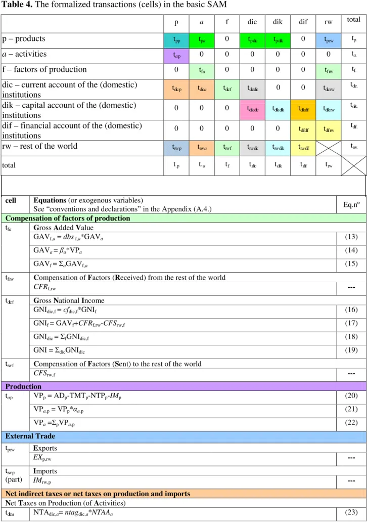
Table 4. The formalized transactions (cells) in the basic SAM
p a f dic dik dif rw total
p – products tp p tp a 0 tp dic tp dik 0 tp rw tp.
a – activities ta p 0 0 0 0 0 0 ta .
f – factors of production 0 tf a 0 0 0 0 tf rw tf .
dic – current account of the (domestic)
institutions tdic p tdic a tdic f tdic dic 0 0 tdic rw
tdic .
dik – capital account of the (domestic)
institutions 0 0 0 tdik dic tdik dik tdik dif tdik rw
tdik .
dif – financial account of the (domestic)
institutions 0 0 0 0 0 tdif dif tdif rw
tdif .
rw – rest of the world trw p trw a trw f trw dic trw di k trw dif trw.
total t.p t.a t.f t.dic t.dik t.dif t.rw
cell Equations (or exogenous variables)
See “conventions and declarations” in the Appendix (A.4.) Eq.nº
Compensation of factors of production
tf a Gross Added Value
GAVf,a = dbsf,a*GAVa (13)
GAVa = a*VPa (14)
GAVf = aGAVf,a (15)
tf rw Compensation of Factors(Received) from the rest of the world
CFRf,rw ---
tdic f Gross National Income
GNIdic,f = cfdic,f*GNIf (16)
GNIf = GAVf+CFRf,rw-CFSrw,f (17)
GNIdic = fGNIdic,f (18)
GNI = dicGNIdic (19)
trw f Compensation of Factors (Sent) to the rest of the world
CFSrw,f ---
Production
ta p VPp = ADp-TMTp-NTPp-IMp (20)
VPa,p = VPp* a,p (21)
VPa = pVPa,p (22)
External Trade
tp rw Exports
EXp,rw ---
trw p (part)
Imports
IMrw,p ---
Net indirect taxes or net taxes on production and imports
Net Taxes on Production (of Activities)
- 14 -
cell Equations (or exogenous variables)
See “conventions and declarations” in the Appendix (A.4.) Eq.nº
NTAdic= aNTAdic,a (24)
NTAa= dicNTAdic,a (25)
trw a NTArw,a= ntarwrw,a*NTAAa (26)
NTArw= aNTArw,a (27)
NTA = dicNTAdic+NTArw (28)
Net Taxes on Products
tdic p NTPdic,p= ntpgdic,p*NTPp (29)
NTPdic= pNTPdic,p (30)
trw p (part)
NTPrw,p= ntprwrw,p*NTPp (31)
NTPrw = pNTPrw,p (32)
NTPp = tpp*DTp (33)
NTP = dicNTPdic +NTPrw (34)
Trade and Transport Margins
tp p TMp,p = tmrp,p*DTp (35)
TMPp = p TMp,p (column sum) (36)
Domestic Trade
DTmpp = VICp + FCp + GCFp (37)
DTp = DTmpp - TMPp - NTPp (38)
tp a (Value of) Intermediate Consumption
VICa = a*VPa (39)
VICp,a = icpp,a*VICa (40)
VICp= aVICp,a (41)
VIC = p aVICp,a (42)
tp dic Final Consumption
FCdic = apcdic* DIdic (43)
FCp,dic = fcsp,dic*FCdic (44)
tp dik Gross Capital Formation
GCFp,dik = gfcfp,dik*P51dik + P52p*chinvp,dik + advp,dik*P53dik (45)
GCFdik = p GCFp,dik (46)
P52p = chinvcp*ASp (47)
P53dik = advcdik*Sdik (48)
Current Transfers
tdic dic CTdic,dic= d5sdic,dic*D5dic + d61sdic,dic*D61dic +d62sdic,dic*D62Pdic + d7dic,dic*D7Pdic +D8dic,dic (49)
D5dic = tidic*AIdic (50)
D61dic = scdic*GNIdic (51)
CTRdic = dic CTdic,dic (52)
CTPdic= dic CTdic,dic (53)
tdic rw CTdic,rw = D5RWdic,rw + D61RWdic,rw + D62RWdic,rw +D7RWdic,rw (54)
trw dic CTrw,dic = d5rwsrw,dic*D5dic + d61rwsrw,dic*D61dic + d62rwsrw,dic *D62Pdic +d7rwsrw,dic *D7Pdic (55)
- 15 -
cell Equations (or exogenous variables)
See “conventions and declarations” in the Appendix (A.4.) Eq.nº
Capital Transfers
tdik ik KTdik,dik = d91dik,dik *D91Pdik +D92Rdik*d92dik,dik + D99Rdik*d99dik,dik (57)
D91Pdik = tkdik * D99Rdik (58)
D92Rdik = cgfcf dik*P51dik (59)
KTRdik = dikKTdik,dik (60)
KTPdik = dikKTdik,dik (61)
tdik rw KTdik,rw = D92Rdik *d92rwdik,rw + D99Rdik*d99rwdik,rw (62)
trw di k KTrw,dik = D92Prw,dik+ D99Prw,dik + K2 rw,dik (63)
Gross Saving
tdik dic Sdik,dic = sidik,dic*Sdic (64)
Sdik = dikSdik,dic (65)
Sdic = (1-apcdic)*DIdic (66)
S = dic Sdic = dik Sdik (67)
Financial Transactions
tdif dif FTdif ---
tdif rw FTRWdif,rw = FTrw,dif + NLBdif (68)
trw dif FTrw,dif ---
Net borrowing/lending
tdik dif NLBdik,dif = AINVdik – (Sdik +KTRdik+KTdik,rw) (69)
NLBdif = dik NLBdik,dif (70)
Row totals
tp. Aggregate Demand
ADp = VICp + FCp + GCFp + EXp,rw (71)
ta . Production Value
VPTa= pVPap (72)
tf . Aggregate Factors Income (Received)
AFIRf = GAVf + CFRf,rw (73)
tdic . Aggregate Income
AIdic = GNIdic + NTAdic + NTPdic + CTRdic +CTdic,rw (74)
tdik . Investment Funds
INVFdik = Sdik+ KTRdik + NLBdik,dif + KTdik,rw (75)
tdif . Total Financial Transactions (Received)
TFTRdif = FTdif,dif + FTRWdif,rw (76)
trw . Value of Transactions to the Rest of the World (Paid)
TVRWPrw = CFSrw,f + aNTArw,a+ p(NTPrw,p + IMrw,p) + dic (CTrw,dic+ FCrw,dic) + dikKTrw,dik + FTrw,dif
(77)
Column totals
t.p Aggregate Supply
ASp = VPp + TMTp + NTPp + IMrw,p (78)
t.a Total Costs
VCTa = GAVa + VICa+ NTAa + NTArw,a (79)
t.f Aggregate Factors Income (Paid)
- 16 -
cell Equations (or exogenous variables)
See “conventions and declarations” in the Appendix (A.4.) Eq.nº
t.dic Aggregate Income
AIPdic = FCdic + CTPdic + Sdic + (CTrw,dic+ FCrw,dic) (81)
t.dik Aggregate Investment
AINVdik = GCFdik + KTPdik + KTrw,dik (82)
tdif . Total Financial Transactions (Paid)
TFTPdif = NLBdif+ FTdif,dif + FTrw,dif (83)
t.rw Value of Transactions from the Rest of the World (Received)
TVRWRrw = CFRf,rw + pEXp,rw+ dicCTdic,rw+ dik KTdik,rw+ FTRWdif,rw (84)
Sources: Santos (2008 and 2009)
As mentioned above, the results of the application of a SAM to Portugal in 2005 are presented in
Section 3. In that application, a scenario (MM) was studied based on a 1% reduction in the rate of
the direct taxes paid by households to the government. In this case, in equation (50), tidich was
changed and the model was subsequently run, with a “new” SAM being calculated, from which it
was possible to make the analysis shown in Section 3.
2.2.3. Accounting multipliers and the master model
Comparing the two described above SAM algebraic versions, besides the common assumptions
referred to at the beginning of Section 2.2, the existence of many fixed parameters in the master
model and fixed average expenditure propensities in the multipliers can be considered to be
amongst its strongest and most limitative assumptions.
Special mention should be made of the financial transactions and of the transactions with the rest of
the world: all of these are considered as exogenous in the accounting multipliers and almost all of
them are considered as exogenous in the master model.
On the other hand, using the methodology of multipliers, shocks can only be performed on matrix X
(transactions between exogenous and endogenous accounts - injections from first into second) and
therefore the account of origin of the flow to be studied has to be set as exogenous. This means that,
at the level of that account, all that can be measured is the direct influence of that shock. The global
effect of the same shock on the destination is not considered. This does not happen with the master
model, with which shocks can be performed using specific parameters (and exogenous variables)
within specific SAM cells and not within SAM accounts. Therefore, more impacts can be measured
- 17 -
3. From the snapshot of the reality under study to alternative scenarios for the measurement
of the impact of socioeconomic policy. An application to Portugal.
The information given by the numerical version of the SAM will now be used to define the
framework for explaining the reality under study. This numerical version will be the one described
in Section 2.1, which represents the reality under study.
The numerical versions replicated after running the SAM-based models that are representative of
the two algebraic versions presented in Section 2.2 – the accounting multipliers (AC) and the
master model (MM) – will represent the two scenarios to be studied and compared with the reality
under study.
In discussing our application of a SAM to Portugal in 2005, the former will be referred to as
“Portugal-05” and the latter as “Scenario-AC” and “Scenario-MM”. As has already been said, these
two alternative scenarios represent the impacts of a policy measure consisting of a 1% reduction in
the rate of the direct taxes paid by households to the government.
Although the modelling methodology adopted can be used to study structural changes, it does not,
however, actually produce structural changes. Therefore, structural aspects will be presented in the
analysis of the “real” SAM (Portugal-05) and will be used to explain some of the impacts in the
constructed scenarios (Scenario-AC and Scenario-MM). As mentioned above, our attention will be
focused on the institutional sectors and the corresponding distribution, redistribution and use of
income. This will involve pursuing the stated aim of studying the SAM-based approach and its use
in defining a suitable framework for explaining the socioeconomic reality of countries and
supporting the policy decision process.
The following analysis will focus on three main aspects: domestic production, domestic demand
and income. The snapshot made of the reality under study will involve the consideration of
questions which the numerical SAM can answer. Thus, using the information provided by the
application already mentioned, our analysis will be based on the specific parts of the SAM (Table
A.2) compiled in tables whose titles are precisely those questions. Some of these tables are
complemented by further information drawn from the integrated economic accounts (Table A.5),
which is not found in this version of the SAM but is included in the author’s research agenda, as
mentioned in Section 4. To support the analysis of those Tables, charts were also constructed. Our
exercise will involve a high level of aggregation, but, as mentioned in Section 2.1, greater
disaggregation is possible, enabling us to answer the same type of questions (or even other
- 18 -
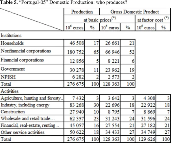
Table 5. “Portugal-05” Domestic Production: who produces?
Sources: Tables A.2 and A.5.
(*)
See the specification of these two types of valuation in the footnote to Table 2.
Source: Table 5
- 19 -
Table 6. “Portugal-05” Domestic Production: at what costs?
Sources: Tables A.2 and A.5. Source: Table 5
- 20 -
Chart 3. “Portugal-05” Domestic Production by Institutional Sectors: at what costs?
Chart 4. “Portugal-05” Domestic Production by Activity Sectors: at what costs?
- 21 -
[See the parts relating to “institutions” in Tables 5 and 6 (and Charts 1 and 3)]
Non-financial corporations are responsible for 65% of domestic production and 52% of the gross
domestic product (the difference between domestic production and intermediate consumption).
Therefore, the cost structure of that institutional sector, namely the importance of intermediate
consumption, contributes significantly towards the reduction of its relative importance in the
economy as a whole, when we pass from domestic production to the gross domestic product. This
does not happen either with the households or with the government – the two other institutional
sectors that make an important contribution to domestic production and the gross domestic product.
In fact, because these two institutional sectors do not require such high proportions of intermediate
consumption in order to produce, their contribution to the gross domestic product (households:
21%; government: 19%) is greater than it is to domestic production (households: 17%; government:
11%). However, in order to produce, they incur higher costs in terms of the compensation of
factors, namely: 49% of the compensation of own account labour and capital, in the case of
households; 71% of the compensation of employees, in the case of the government – but this does
not affect their relative shares of domestic production and the gross domestic product. These are
aspects that cannot yet be seen in the structure of the SAM used in this paper, but which will
become visible in the future, as a result of what will be mentioned in Section 4.
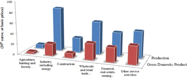
[See the parts relating to “activities” in Tables 5 and 6 (and Charts 2 and 4)]
Industry, including energy5, is responsible for 30% of domestic production and for 18% of the gross
domestic product. Thus, although this activity has the highest share of domestic production, due to
the importance of intermediate consumption (73%) in the structure of its production costs, of the six
sectors of activity into which the economy as a whole is organised, it is only the fourth most
important activity in terms of its contribution to the gross domestic product. In turn, other service
5
- 22 -
activities6 are responsible for only 18% of domestic production, but have the highest share in terms
of the gross domestic product: 27%. The compensation of factors made the major contribution to
the structure of production costs, most notably the compensation of employees. Wholesale and
retail services, repair of motor vehicles and household goods, hotels and restaurants, transport and
communications were in a similar situation to the other service activities.
The above analysis (supported by Tables 5 and 6 and the corresponding charts) was based on values
at basic prices, i.e. including net taxes on production. However, the relative positions of the various
activities are not significantly different if we consider the gross domestic product at factor cost (in
Table 5).
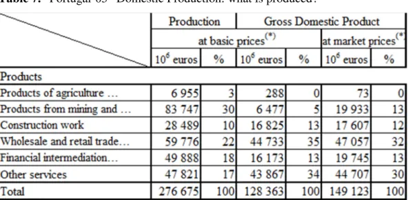
Table 7. “Portugal-05” Domestic Production: what is produced?
Source: Table A.2.
(*)
See the specification of these two types of valuation in the footnote to Table 2.
6
- 23 - [See Tables 7 and 5 and Charts 5 and 2]
Due to the way in which the products are organised and their underlying nomenclatures, a close
relationship can be established between what is produced and the sectors of activity that produce
these products. Thus, the products mainly produced by industry (including energy), i.e. the products
from mining and quarrying, manufactured products and energy products7, are the most
representative group of the six considered, accounting for 30% of domestic production, and yet, at
the same time, they are the least representative in terms of the gross domestic product (at basic
prices), being responsible for only 5%. However, with the help of net taxes on products, this same
group regains its importance, being responsible for 13% of the GDP (gross domestic product) at
market prices. In turn, wholesale and retail trade services, repair services, hotel and restaurant
7
Products included in this group: metal ores; other mining and quarrying products; food products and beverages; tobacco products; textiles; wearing apparel; furs; leather and leather products; wood and products of wood and cork (except furniture), articles of straw and plaiting materials; pulp, paper and paper products; printed matter and recorded media; coke, refined petroleum products and nuclear fuel; chemicals, chemical products and man-made fibers; rubber and plastic products; Other non-metallic mineral products; basic metals; fabricated metal products, except machinery and equipment; machinery and equipment n.e.c.; office machinery and computers; electrical machinery and apparatus n.e.c; radio, television and communication equipment and apparatus; medical, precision and optical instruments, watches and clocks; motor vehicles, trailers and semi-trailers; other transport equipment; furniture; other manufactured goods n.e.c.; recovered secondary raw materials; electrical energy, gas, steam and hot water; collected and purified water, distribution services of water (Santos, 2009: 146-147). Products that were not produced in Portugal in 2005 are not mentioned.
Chart 5. “Portugal-05” Domestic Production: what is produced?
- 24 -
services, and transport and communication services8, are the second most important group in terms
of domestic production, with 22% of the total and occupy first position in terms of the gross
domestic product at both basic prices and market prices, with 35% and 32% of the total,
respectively.
Financialintermediation services, real estate, rental and business services9 and other services, have
almost similar shares in domestic production, with 18% and 17% of the total, respectively.
However, the other services occupy second position in the gross domestic product at basic prices
and at market prices, with 34% and 30% of the total, respectively, whereas financialintermediation
services, real estate, rental and business services has a share of only 13%, in both cases.
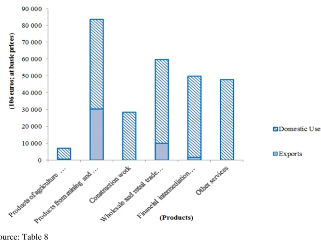
Table 8. “Portugal-05” Domestic Production: what destination?
Source: Table A.2.
8
Products included in this group: trade, maintenance and repair services of motor vehicles and motorcycles; retail trade services of automotive fuel; wholesale trade and commission trade, except of motor vehicles and motorcycles; retail trade, except of motor vehicles and motorcycles; repair of personal and household goods; hotels and restaurants; land transport; transport via pipelines; water transport; air transport; supporting and auxiliary transport activities; activities of travel agencies; post and telecommunications (Santos, 2009: 146-147).
9
- 25 -
Chart 6. “Portugal-05” Domestic Production: what destination?
Source: Table 8
[See Table 8 and Chart 6]
85% of domestic production is used internally, with the remaining 15% being exported. Most of the
exported products come from mining and quarrying, manufactured products and energy products,
which are also the most representative in domestic production, as seen above.
Table 9. “Portugal-05” Domestic Demand: what origin?
- 26 - [see Table 9 and Chart 7]
The domestic production used internally is valued at basic prices, but, after being valued at market
prices (i.e. when the net taxes on products are added to the basic prices), it satisfies 83% of
domestic demand, with the remaining 17% being satisfied by imports.
Besides being the most exported products, products from mining and quarrying, manufactured
products and energy products are also the most imported ones, since 35% of domestic demand is
not satisfied by products with domestic origin. On the other hand, although the products of
agriculture, hunting, forestry, fisheries and aquaculture need to be imported to satisfy 21% of
domestic demand, this relative importance does not exist in absolute terms. Chart 7.“Portugal-05” Domestic Demand: what origin?
- 27 -
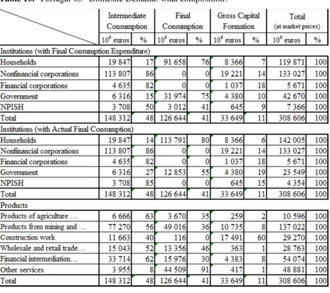
Table 10. “Portugal-05” Domestic Demand: what composition?
Sources: Tables A.2 and A.5.
Chart 8. “Portugal-05” Domestic Demand by Institutional Sectors: what composition?
- 28 - [See Table 10 and Charts 8 and 9]
Intermediate and final consumption account for almost all of the domestic demand (48% and 41%
respectively), whereas gross capital formation represents the remaining 11%. Intermediate
consumption accounts for 86% of the demand of non-financial corporations and 82% of the demand
of financial corporations, while more than half of the demand for four of the six groups of products
is put to the same use. The two groups of products whose demand composition does not have its
main share in intermediate consumption are construction work, where 60% of demand is for gross
capital formation, including acquisitions net of disposals of dwelling by households, and other
services, where 91% of demand is for final consumption.
Some differences can be identified in the amounts and composition of the demand of households,
the government and the NPISH, depending on whether we consider final consumption expenditure
or the actual final consumption. Thus, final consumption expenditure is, respectively, 76%, 75%
and 41% of total demand in the case of those three institutional sectors and (in the same order) that
share changes to 80%, 55% and 0% of total demand if we consider the actual final consumption.
Therefore, when households receive social transfers in kind from the government and the NPISH,
the part of (actual) final consumption in the total demand of households increases by four
percentage points. In turn, the corresponding parts of the government and of the NPISH decrease by
twenty percentage points and forty-one percentage points, respectively.
Chart 9. “Portugal-05” Domestic Demand by Products: what composition?
- 29 -
Table 11. “Portugal-05” National Income: what origin and distribution?
Sources: Tables A.2 and A.5.
[See Table 11 and Chart 10]
The gross domestic product (at market prices), which is also the gross domestic income, becomes
national income after the primary income generated in the domestic economy by non-residents is
deducted and the primary income generated abroad by residents is added to the amount. This
generated primary income includes the compensation of labour (employees), own account labour
and capital, and the net indirect taxes (or net taxes on products and production), which take into
account the valuation of the gross domestic product and the compensation of the government. Thus,
more than half of national income is compensation of labour, which is received entirely by Chart 10. “Portugal-05” National Income: what origin and distribution?
- 30 -
households, contributing to the share of 73% of the total gross national income received by that
institutional sector, jointly with the compensation of own account labour and capital. The remaining
27% of the gross national income, or of the income generated by residents (in the economy and in
the rest of the world), is distributed to the government (13%), non-financial corporations (10%),
financial corporations (3%) and NPISH (1%). What is really quite curious is the distribution of net
national income (the gross national income minus the consumption of fixed capital), especially the
share of non-financial corporations, which are responsible for 65% of domestic production, and
whose 10% share of gross national income is reduced to 1% when the depreciation of fixed capital
is considered.
Since both the amounts and the significance of the consumption of fixed capital have not been
sufficiently studied by the author, our analysis will continue in gross terms.
Table 12. “Portugal-05” Income in Cash: what origin and distribution?
- 31 - [See Table 12 and Chart 11]
By adding the current and capital transfers to the gross national income, we were able to calculate
the so-called income in cash, whose origin and distribution by institutional sectors can be seen in
Table 1210. Thus, 59% of the total income in cash is accounted for by households, 75% of which
originates from gross national income, 23% from current transfers and 2% from capital transfers.
The government has the second most important share of that income, namely 27% of the total, 64%
of which originates from current transfers and 30% from gross national income. The remainder is
distributed among the other three institutional sectors: 8% for non-financial corporations, 5% for
financial corporations and 2% for NPISH.
10
Tables A.6.1 and A.6.2, in the appendix, show the links between gross national income and income in cash through gross disposable income.
Chart 11. “Portugal-05” “Portugal-05” Income in Cash: what origin and distribution?
- 32 -
Table 13. “Portugal-05” Cash Needs: what origin and distribution?
Source: Table A.2.
[See Table 13 and Chart 12]
The institutional sectors require income for consumption and investment purposes, as well as for
transfer, this will be the so-called cash needs. Thus, if the income in cash is not sufficient to satisfy
those requirements, the institutional sectors will have net borrowing; otherwise, they will have net
lending.
Households account for 54% of the cash needs by the institutions as a whole, 67% of which is used
for final consumption. The government is the second institutional sector that requires more income
(29% of the total), 46% of which is used to pay current transfers and 44% for final consumption
(most of which will be used for the actual final consumption of households, as was seen above). Chart 12. “Portugal-05” Cash Needs: what origin and distribution?
- 33 -
Non-financial corporations, with an 11% share of the cash needs of the whole economy, represent
the institutional sector that invests most, in other words that spends most on gross capital formation.
However, as can be seen in Table A.6.3 (in the appendix), although 98% of the gross capital
formation of non-financial corporations is gross fixed capital formation, 74% is used to cover the
consumption of fixed capital and only 25% is used for net fixed capital formation.
Table 14. “Portugal-05” Net Lending or Net Borrowing?
Source: Table A.2.
Chart 13. “Portugal-05” Net Lending or Net Borrowing?