Lat. Am. j. solids struct. vol.10 número3

(1)

Abstract

Steel and composite (steel-concrete) highway bridges are currently subjected to dynamic actions of variable magnitude due to convoy of vehicles crossing on the deck pavement. These dynamic actions can generate the nucleation of fractures or even their propagation on the bridge deck structure. Proper consideration of all of the aspects mentioned pointed our team to develop an analysis meth-odology with emphasis to evaluate the stresses through a dynamic analysis of highway bridge decks including the action of vehicles. The design codes recommend the application of the curves S-N associated to the Miner’s damage rule to evaluate the fatigue and service life of steel and composite (steel-concrete) bridges. In this work, the developed computational model adopted the usual mesh refinement techniques present in finite element method simula-tions implemented in the ANSYS program. The investigated highway bridge is constituted by four longitudinal composite gird-ers and a concrete deck, spanning 40.0m by 13.5m. The analysis methodology and procedures presented in the design codes were applied to evaluate the fatigue of the bridge determining the ser-vice life of the structure. The main conclusions of this investiga-tion focused on alerting structural engineers to the possible distor-tions, associated to the steel and composite bridge’s service life when subjected to vehicle’s dynamic actions.

Key words

dynamic analysis, fatigue assessment, structural dynamics, steel and composite (steel-concrete) highway bridges, design codes, computational modelling.

Fatigue analysis and life prediction of composite

high-way bridge decks under traffic loading

1 INTRODUCTION

Steel and composite (steel-concrete) highway bridges are usually subjected to dynamic actions of variable magnitude due to convoy of vehicles crossing on the deck pavement. Depending on the magnitude and intensity of these dynamic actions, these adverse effects may compromise the struc-tural system response reliability that could also lead to a reduction of the expected bridge service life [1-3].

Fe rn an do N . Le itão1,

Jos é Gu ilh erm e S. da Silva2,*, Se b as tião A. L. d e An drad e3

1_{Post-graduate Programme in Civil}

Engineer-ing, PGECIV, State University of Rio de Janeiro, UERJ, Brazil

2_{Structural Engineering Department, State}

University of Rio de Janeiro, UERJ, Brazil

3_{Civil Engineering Department, Pontifical}

Catholic University of Rio de Janeiro, PUC-Rio, Brazil

Received 08 Fev 2012 In revised form 18 Oct 2012

(2)

Latin American Journal of Solids and Structures 10(2013) 505 – 522

Proper consideration of all of the aspects earlier mentioned pointed our team to develop an analysis methodology with emphasis to evaluate the stresses through a dynamic analysis of steel and compo-site (steel-concrete) highway bridge decks, including the action of vehicles crossing on the pavement surface [1-4].

The present investigation utilises techniques for counting stress-cycles and for applying cumula-tive damage rules combined with S-N curves. The first steps of the composite highway bridge study involved an extensive literature review of the techniques used to define steel and composite bridges service life, a study of the theoretical aspects of fatigue in steel, and the recommended procedures present in main steel and composite structural design codes [5,6].

The design codes recommend the adoption of the S-N curves associated with the Miner’s damage rule to evaluate the steel and composite bridges fatigue and service life. These codes also recom-mend that the bridge structure designs should avoid local stress concentrations, to prevent possible fatigue points.

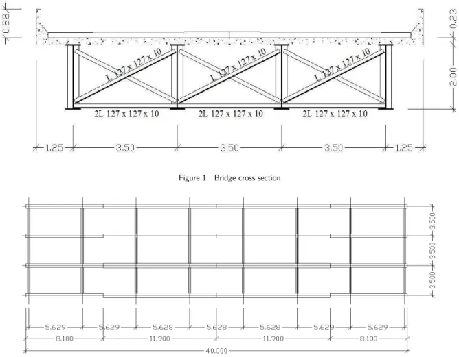
The investigated composite bridge has a roadway width of 12.50m and a concrete deck thickness of 0.23m, spanning 40.0m by 13.5m. The structural system consists of four longitudinal composite girders and a concrete deck. The computational model used in the composite bridge dynamic analy-sis, adopts the usual mesh refinement techniques present in finite element method simulations im-plemented in the ANSYS program [7].

The beam steel sections were simulated by three-dimensional beam and shell finite elements. The beam web was represented by shell finite elements. The top and bottom beam flanges and the lon-gitudinal and vertical stiffeners were simulated by three-dimensional beam elements considering flexural and torsional effects. The bridge concrete slab was simulated by shell finite elements.

The proposed analysis methodology and the procedures presented in the design codes [5,6] were used to evaluate the bridge fatigue response in terms of its structural service life. The main conclu-sions of this paper focused on alerting structural engineers to the possible distortions related to the bridge’s service life when subjected to vehicle’s dynamic actions.

2 MATHEMATICAL MODEL

2.1 Bridge Deck Structural Model

The structural model investigated in the present study corresponds to a composite (steel-concrete) highway bridge deck with straight axis, simple supported, spanning 13.0m by 40.0m. The structural system is constituted of four composite girders and a 0.225m thick concrete slab, as shown in Fig-ures 1 to 4.

The steel sections used were welded wide flanges (WWF) made with a 350MPa yield stress steel

grade and 485MPa ultimate strength. A 2.05x105MPa Young’s modulus was adopted for the steel

beams. The concrete slab possesses a 25MPa specified compression strength and a 3.05x104MPa

(3)

Figure 1 Bridge cross section

Figure 2 Bridge top view

Figure 3 Three-dimensional bridge view

(4)

Table 1 Geometrical characteristics of the beam steel sections.

Cross Section Extremity Cross Section: geometric properties (mm)

Height (d) 2000

Top flange width (bs) 450

Top flange thickness (ts) 25

Bottom flange width (bi) 450

Bottom flange thickness (ti) 50

Web thickness (tw) 9.5

Central Cross Section: geometric properties (mm)

Height (d) 2000

Top flange width (bs) 500

Top flange thickness (ts) 25

Bottom flange width (bi) 670

Bottom flange thickness (ti) 50

Web thickness (tw) 9.5

2.2 Vehicle Model

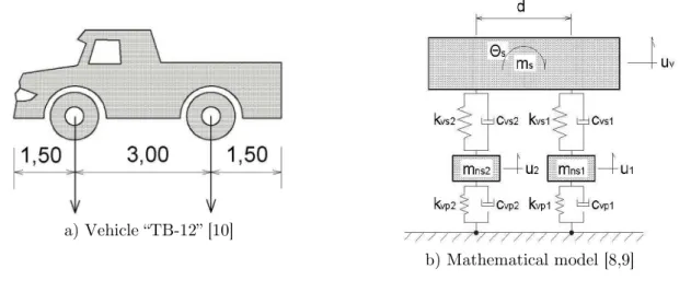
In this work, the adopted vehicle mathematical model was developed by Almeida [8,9]. This model is considered discrete and constituted by “mass-spring-damper” systems with three masses and a four freedom degree. The vehicle model was based on the NBR 7188 [10] vehicle “TB-12” and con-sists of a three masses model with four degrees of freedom (three translational and one rotational) and two axles to simulate each single vehicle, as presented in the Figure 5. Translational vertical displacements and rotational displacements are considered in the vehicle model.

Figure 5 illustrates this representation and uses the following notation: uv, is the vehicle vertical

displacement of the suspended mass; θs, is the vehicle rotational displacement related to the

sus-pended mass; u1 and u2 are the vehicle vertical displacements of the non-suspended mass; ms is the

vehicle suspended mass; mns is the vehicle ith non-suspended mass (for each axle), respectively; kvs

and kvp are the ith stiffness coefficients related to vehicle suspension and tires (for each axle),

respec-tively; cvs and cvp are ith the damping coefficients related to vehicle suspension and tires (for each

axle), respectively.

The vehicle natural frequencies oscillating on rigid base (vertical motion), corresponding to the vehicle suspended mass (suspension system) and non-suspended mass degrees of freedom (tires), as presented in Figure 5, were made equal to 3.0Hz and 20.0Hz, respectively [8,9]. However, the vehicle model has a lower natural frequency, associated to the vehicle suspended mass (suspension system) degree of freedom which is equal to 2.3Hz (rotational motion).

The relative damping coefficient of the vehicles vibration mode with predominant movement of

the vehicles suspended mass is assumed to be ξ=0.1 (ξ=10%) [8,9]. The total mass used in this

vehicle model is equal to 12t (ms = 10.667kg; mns1 = 666.5kg and mns1 = 666.5kg), corresponding to

(5)

a) Vehicle “TB-12” [10]

b) Mathematical model [8,9]

Figure 5 Vehicle model.

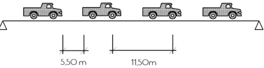
2.3 Semi-infinite Train of Vehicles

The moving load is modelled by an infinite series of equal vehicles, regularly spaced, and running at

constant velocity, υ. If l is the distance between two successive vehicles and as these cars enter one

by one into the bridge deck, it is created a time repeated movement variation governed by the

fre-quency, ft = υ/l, associated with the movement of the vehicles on the bridge, which can be called

traversing frequency [3].

After a certain time period, t1, denominated crossing period, the first vehicle in the train reaches

the far end of the bridge and from this instant, on the total mass of the vehicles on the bridge mains practically constant. Under these conditions the bridge will soon reach a steady-state re-sponse situation, which includes repetition of maximum values directly related to the fatigue and the service life of the structure [3], as illustrated in Figures 6 to 8.

Figure 6 Two vehicles crossing the bridge: υ = 80km/h and l = 22m (Load Model I - LM-I).

(6)

Figure 8 Four vehicles crossing the bridge: υ = 60km/h and l = 11.50m (Load Model III - LM-III).

2.4 Structural Damping

In this work, the structural damping was considered according to the Rayleigh proportional

damping formulation [11]. The bridge structure damping matrix is defined by the parameters α

and β, determined in function of the damping modal coefficient. According to this formulation

[11], the structural system damping matrix [C] is proportional to the mass and stiffness matrix, as shown in Equation (1):

[

C

_]

₌

_α

_[

M

_]

₊

_β

_[

K

_]

₍₁₎

The expression above can be rewrite in terms of the modal damping coefficient and the natural frequency, leading to the Equation (2):

ξ

i

=

α

2 ω

i

+

βω

i

2

(2)

Where ξi is the modal damping coefficient and ωi is the natural frequency associated to the

mode shape “i”. Isolating the parameters α and β of the Equation (2) for two natural frequencies,

ω01 and ω02, adopted according to the relevance of the corresponding vibration mode for the

structural system dynamical response, it can be written:

β

₌

2(ξ

2

ω

02

−

ξ

1

ω

01

)

ω

₀₂

ω

₀₂

−

ω

₀₁

ω

₀₁ (3)

α

=

2 _ξ1ω

01

−

βω

01ω01 (4)

With two values of natural frequencies is possible to evaluate the parameters α and β

(7)

tak-Latin American Journal of Solids and Structures 10(2013) 505 – 522

en as the extreme frequencies of the structure spectrum. In this paper the frequency ω01 adopted

will be the structure fundamental frequency and the frequency ω02 considered will be the system

second natural frequency. The modal damping coefficient adopted in this investigation is equal to

0.03 (ξ=3%) [1-3].

3 FINITE ELEMENT MODELLING

3.1 Composite (Steel-Concrete) Bridge Finite Element Model

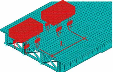
The computational model, developed for the composite bridge dynamic analysis, adopted the usual mesh refinement techniques present in finite element method simulations implemented in the AN-SYS program [7].

The beam steel sections were simulated by three-dimensional beam and shell finite elements. The beam web thickness was represented by shell finite elements (SHELL63 [7]). The beam top and bottom flange and the longitudinal and vertical stiffeners were simulated by three-dimensional beam elements (BEAM44 [7]), where flexural and torsion effects were considered. The bridge con-crete slab was simulated by shell finite elements (SHELL63 [7]).

The computational model used rigid connections like “offsets” in order to guarantee the strain compatibility between plate elements (concrete slab) and three-dimensional beam elements (steel beams), simulating the composite (steel-concrete) highway bridge deck with full interaction.

The final computational model adopted used 4992 nodes, 2264 three-dimensional beam elements and 4324 shell elements, which resulted in a numeric model with 29952 degrees of freedom. In se-quence, Figure 9 illustrates the composite bridge finite element model. Figure 10 illustrates this strategy considering the Load Model I (see Figure 6).

4 DYNAMIC ANALYSIS

4.1 Natural Frequencies and Vibration Modes Analysis

The composite bridge natural frequencies were determined with the aid of the numerical simulations, as presented in Table 2. The associated composite bridge vibration modes are shown in Figure 11. It can be clearly noticed from Table 2 results, that there is a very good agreement between the

fi-nite elements frequencies values and the frequencies obtained by Silva [3] and Murray et al_[12].

(8)

Figure 9 Composite (steel-concrete) highway bridge deck finite element model.

Figure 10 Vehicles crossing the investigated composite bridge.

Table 2 Composite bridge natural frequencies.

Bridge natural frequencies: f0i (Hz) - ANSYS [7] GDYNABT

[3] f01 (Hz)

AISC [12] f01 (Hz)

f01 f02 f03 f04 f05 f06

2.90 3.64 6.87 9.63 11.03 12.85 2.85 2.65

Elements: 6588 Beam elements: 2264 Shell elements:4324 Nodes: 4992

(9)

a) First vibration mode: f01=2.90Hz. _{b) Second vibration mode: f}₀₂_=3.64Hz.

c) Third vibration mode: f03=6.87Hz. d) Fourth vibration mode: f04=9.63Hz.

e) Fifth vibration mode: f05=11.03Hz. f) Sixth vibration mode: f06=12.85Hz.

Figure 11 Composite bridge vibration modes.

4.2 Composite Bridge Dynamic Response

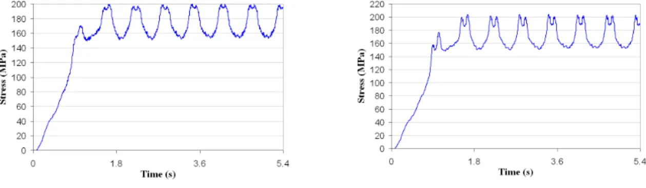
The dynamical analysis proceeded with the evaluation of the composite bridge dynamic response. Three loading cases were investigated: central track passage, lateral track passage and both lateral track passage, see Figures 12 and 13. Figures 14 and 15 illustrate the maximum stresses at the bot-tom flange of the composite beams, associated to flexural effects.

In general, the composite beams sections closer than dynamic loading application track presented higher stress values. In these situations the beams were subjected to higher impacts.

(10)

a) Central track passage. b) Lateral track passage.

c) Both lateral track passage.

Figure 12 Investigated loading cases.

Figure 13 Location where the stresses were obtained on the bridge structure.

a) Beam 1 bottom flange. b) Beam 2 bottom flange.

(11)

a) Beam 1 bottom flange. b) Beam 2 bottom flange.

Figure 15 Stresses due to the LM-II (see Figure 7). Load mobility effect. Two lateral track passage.

On the other hand, the stress values corresponding to beam 4 (see Figure 13), opposite side of the lateral track convoy passage, were very small when compared with other composite beams. This is another important issue to the fatigue analysis due to the fact that the random nature of the dy-namic loadings can make structural elements very loaded or even practically without loading along the time, causing an increase on the stress range.

5 FATIGUE ASSESSMENT

5.1 Cycle Counting and Structural Element Fatigue Class

The stress values obtained in the dynamic analysis, due to load mobility and irregular pavement surface effects, were used to evaluate the fatigue of the bridge determining the service life of the structure. However the analysis of the obtained results is very complex, with a lot of stress peaks and containing diversified values. Thus, the manual stress cycle counting becomes impossible. The peaks and valleys of the presented stress history graphs need to be counted. This investigation used the Rainflow method for stress cycle counting. In order to avoid the manual stress cycle counting a Matlab [13] routine was implemented and validated, based on results found by others authors [1-4].

Fatigue is a localized damage process of a component produced by cyclic loading. It is the result of the cumulative process consisting of crack initiation, propagation, and final fracture of a struc-tural component. To determine the fatigue service life and cumulated damage it is necessary to obtain the stress ranges during the vehicles moving on the bridge structure.

The fatigue strength for nominal stresses is represented by a series of logarithmic curves (S-N curves), which correspond to typical detail categories. An S-N curve defines alternating stress values versus the number of cycles required to cause failure at a given stress ratio. The Y- axis represents the stresses (S) and the X-axis represents the number of cycles (N) [1-6].

In the S-N curves, each detail category is designated by a letter (Categories A through E’) [5] or

a number (Categories 36 to 160) [6], which represents, in N/mm2, the reference value for the

(12)

The design life, related to the reference period of time for which a structure is required to per-form safely with an acceptable probability that failure by fatigue cracking will not occur, has been considered to be 75 years [5] and 120 years [6], respectively, in the overall development of these specifications [5,6].

These values associated with the S-N curves of each design code [5,6] were used to obtain the cumulative damage and respectively the service life of each analysed structural element. It must be emphasized that each design code [5,6] considers different structural details classification. The types of structural details analysed in this work were presented in Table 3.

The bridge steady state response, see Figures 14 and 15, was considered to obtain the maximum stress values due to vehicles traffic on the composite bridge deck. Based on these values, the Rain-flow cycle counting was applied to determine the stress ranges. Each associated stress cycle was

used proportionally with 2 x 106 cycles, which is the design code value for this analysis type [1-6].

5.2 Composite Bridge Service Life

In sequence of the analysis, Tables 4 to 12 illustrate the calculations of the composite bridge service

life (σmax: maximum stresses and Δσmax: stresses maximum variation) when I, II and

LM-III (see Figures 6 to 8) were applied on the bridge structure. The vehicles were considered moving on the central and lateral track passage (see Figures 12 and 13).

Only the dynamic effects related to the load mobility were considered in this analysis. Tables 4 to 12 present the service life results for stress values associated with different structural elements (see Figures 12 and 13). The results were based on design code recommendations and specific S-N curves [5,6].

Table 3 Structural details classification and fatigue class.

Detail Picture Type Design code element fatigue class

AASHTO [5] EUROCODE 3 [6]

1 Weld between

web and flange B 125

2 Cross section

union weld B 125

3 Connectors weld C 80

4 Bottom

(13)

Table 4 LM-I. Central track. Load mobility effect.

Detail Beam σmax

(MPa)

Δσmax

(MPa)

Bridge service life in years AASTHO [5]

75 years* EUROCODE 3 [6] _{120 years*}

1 and 2

1 63.03 12.00 19555.02 19854.81

2 91.03 39.00 1065.71 1082.05

4 63.03 12.00 19555.02 19854.81

3 and 4

1 63.03 12.00 7165.20 4987.30

2 91.03 39.00 390.49 271.80

4 63.03 12.00 7165.20 4987.30

*Minimum bridge service life

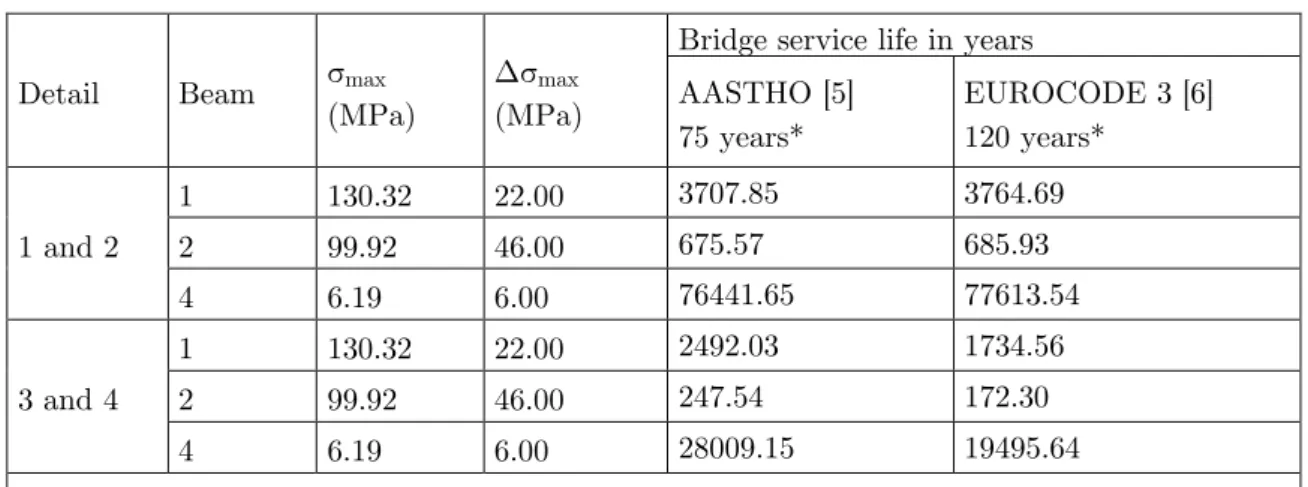
Table 5 LM-I. Lateral track. Load mobility effect.

Detail Beam σmax

(MPa)

Δσmax

(MPa)

75 years*

EUROCODE 3 [6] 120 years*

1 and 2

1 130.32 22.00 3707.85 3764.69

2 99.92 46.00 675.57 685.93

4 6.19 6.00 76441.65 77613.54

3 and 4

1 130.32 22.00 2492.03 1734.56

2 99.92 46.00 247.54 172.30

4 6.19 6.00 28009.15 19495.64

Table 6 LM-I. Both lateral tracks. Load mobility effect.

Detail Beam σmax

(MPa)

Δσmax

(MPa)

75 years*

1 and 2

1 126.74 23.00 6793.52 6897.67

2 132.46 29.00 1457.31 1479.65

4 126.74 23.00 6793.52 6897.67

3 and 4

1 126.74 23.00 2489.23 1732.62

2 132.46 29.00 533.98 371.67

4 126.74 23.00 2489.23 1732.62

(14)

Table 7 LM-II. Central track. Load mobility effect.

Detail Beam σmax

(MPa)

Δσmax

(MPa)

75 years*

1 and 2

1 96.59 11.00 14154.66 14371.66

2 127.95 52.00 567.44 576.14

4 96.59 11.00 14154.66 14371.66

3 and 4

1 96.59 11.00 5186.44 3610.00

2 127.95 52.00 207.92 144.72

4 96.59 11.00 5186.44 3610.00

Table 8 LM-II. Lateral track. Load mobility effect.

Detail Beam σmax

(MPa)

Δσmax

(MPa)

75 years*

1 and 2

1 203.67 47.00 472.34 479.58

2 147.93 46.00 266.39 270.47

4 7.51 4.00 299921.05 304519.00

3 and 4

1 203.67 47.00 173.07 120.47

2 147.93 46.00 97.61 67.94

4 7.51 4.00 109894.74 76491.72

Table 9 LM-II. Both lateral tracks. Load mobility effect.

Detail Beam σmax

(MPa)

Δσmax

(MPa)

75 years*

1 and 2

1 200.36 48.00 406.27 412.49

2 204.28 53.00 167.27 169.83

4 200.36 48.00 406.27 412.49

3 and 4

1 200.36 48.00 148.86 103.61

2 204.28 53.00 61.29 42.66

4 200.36 48.00 148.86 103.61

(15)

Table 10 LM-III. Central track. Load mobility effect.

Detail Beam σmax

(MPa)

Δσmax

(MPa)

75 years*

1 and 2

1 27.28 35.00 296.20 300.74

2 29.67 53.00 71.83 72.93

4 27.28 35.00 296.20 300.74

3 and 4

1 27.28 35.00 108.53 75.54

2 29.67 53.00 26.32 18.32

4 27.28 35.00 108.53 75.54

Table 11 LM-III. Lateral track. Load mobility effect.

Detail Beam σmax

(MPa)

Δσmax

(MPa)

75 years*

1 and 2

1 46.21 43.00 107.52 109.17

2 28.50 46.00 274.98 279.20

4 20.22 11.00 9157.79 9298.18

3 and 4

1 46.21 43.00 39.40 27.42

2 28.50 46.00 100.76 70.13

4 20.22 11.00 3355.53 2335.60

Table 12 LM-III. Both lateral tracks. Load mobility effect.

Detail Beam σmax

(MPa)

Δσmax

(MPa)

75 years*

1 and 2

1 21.29 40.00 124.68 126.59

2 39.33 52.00 173.06 175.72

4 43.10 52.00 133.48 135.53

3 and 4

1 21.29 40.00 45.68 31.80

2 39.33 52.00 63.25 44.03

4 43.10 52.00 48.91 34.04

(16)

The stress values obtained in the dynamic analysis due to load mobility was used to evaluate the fatigue performance of the investigated composite bridge measured in terms of its service life. How-ever, the analysis of the results is very complex, with numerous stress peaks of diversified magni-tudes.

Thus, manual stress cycle counting is, for these structures, an impossible task. This way, the pre-sent investigation adopts the Rainflow method for stress cycle counting. In order to avoid the man-ual stress cycle counting approach, a Matlab [13] routine was developed, implemented and validated, based on results presented by others authors [1-4].

The results presented in Tables 4 to 12, related to the three loading cases I, d II and LM-III (see Figures 6 to 8), indicated that the investigated composite (steel-concrete) highway bridge will perform safely with an acceptable probability that indicates that a failure by fatigue cracking will not occur.

In fact, in most of the analysed cases, the composite bridge service life values were higher than those proposed by the design codes [5,6], ensuring that the members, connections and joints sub-jected to dynamic actions related to the load mobility effects will not failure by fatigue cracking. However, when the lateral track path (LM-II, see Figures 7 and 12) and two simultaneous lateral track paths (LM-III, see Figures 8 and 12) dynamic actions were applied on the investigated struc-tural system, it was concluded that the service life values proposed by the design codes [5,6] were surpassed in some specific situations, see Tables 8 to 12.

Another important aspect is the influence of the dynamic load position. In this investigation, when the loading situation was associated to the convoy of vehicles moving on the bridge lateral track passage the stress values and also stress ranges were higher than those obtained when compared to those provided by vehicles moving on the bridge central track passage. This conclusion emphasizes the importance to consider the contribution of torsional vibrations modes in the composite (steel-concrete) highway bridge dynamical analysis.

It was observed that when the vehicles convoy is moving on the bridge left lateral track, some structural elements, near the dynamic loading position, presented high stress values, while the other structural elements presented small stress values. This alternation in the stress values produced a significant influence on the stress range.

6 FINAL CONSIDERATIONS

In this investigation, an analysis methodology was presented to evaluate the fatigue of the steel and composite highway bridges in terms of the structural system service life. The composite bridge ser-vice life results corroborated the importance of considering the roughness of the pavement surface and other design parameters like: floor thickness, structural damping and beam cross section geo-metrical properties in the bridge dynamic and fatigue analysis.

(17)

The investigated composite (steel-concrete) highway bridge will perform safely with an accepta-ble probability that indicates that failure by fatigue cracking will not occur. The structural system service life values were higher than those proposed by the design codes [5,6], ensuring that the members, connections and joints will not failure by fatigue cracking.

However, when the dynamic actions related to the vehicles moving on the bridge lateral track path and two simultaneous lateral track paths were applied on the bridge structure, it was observed that the service life values proposed by the design codes [5,6] were surpassed in some specific situa-tions.

On the other hand, when the loading situation was associated with the vehicles moving on the bridge lateral track path, the stress values and stress ranges were higher than those obtained with the results related to the case of vehicles moving on the bridge central track path. It could also be concluded that the contribution of torsional vibration modes presented influence on the composite (steel-concrete) highway bridge dynamic and fatigue analysis.

The analysis methodology presented in this paper is general and is the author intention to use this solution strategy on other highway bridge types such as: multigirder bridges, continuous multi-girder bridges, cable-stayed bridges, slant-legged rigid-frame bridges, and so forth. The fatigue prob-lem is certainly much more complicated and is influenced by several highway bridge types. Further research in this area is currently being carried out.

Acknowledgements The authors gratefully acknowledge the financial support for this work provided by the Brazilian Science Foundations CAPES, CNPq and FAPERJ.

References

[1] Leitão, F.N., “Fatigue Analysis of Composite Highway Bridges”, MSc Dissertation (In Portuguese). Civil Engi-neering Post-graduate Programme, PGECIV. State University of Rio de Janeiro, UERJ, Rio de Janeiro, Brasil, 2009.

[2] Leitão, F.N.; Silva, J.G.S. da; Andrade, S.A.L. de; Vellasco, P.C.G. da S.; Lima, L.R.O. de. “Fatigue Analysis of Composite (Steel-Concrete) Highway Bridges Subjected to Dynamic Actions of Vehicles”. CC 2011 - The Thirteenth International Conference on Civil, Structural and Environmental Engineering Computing. Civil-Comp Press. Chania, Crete, Greece. Vol. 1. pp. 1-17, 2011.

[3] Silva, J.G.S. da, “Dynamical Performance of Highway Bridge Decks with Irregular Pavement Surface”. Com-puter & Structures, 82 (11-12), 871-881, 2004.

[4] Pravia, Z.M.C., “Steel Bridge Structures with Crack Stability”. DSc Thesis (In Portuguese). COPPE/UFRJ, Rio de Janeiro, RJ, Brasil, 2003.

[5] AASHTO. LRFD Bridge Design Specifications. American Association of State High-way and Transportation Officials, Washington, USA, 2005.

[6] EUROCODE 3. Design of Steel Structures. European Committee for Standardisation. Bruxelas, 2003.

(18)

[8] Almeida, R. S. de, “Vibration Analysis of Highway Bridges due Vehicle Traffic on Roughness Pavement Sur-face”. MSc Dissertation (In Portuguese). Civil Engineering Post-graduate Programme, PGECIV, State Univer-sity of Rio de Janeiro, UERJ, Rio de Janeiro, Brazil, 2006.

[9] Almeida, R. S. de and Silva, J.G.S. da, “A Stochastic Modelling of the Dynamical Response of Highway Bridge Decks Under Traffic Loads”. ECCM 2006 - III European Conference on Computational Mechanics, 2006. [10] NBR 7188. Carga Móvel em Ponte Rodoviária e Passarela de Pedestre. Associação Brasileira de Normas

Téc-nicas, Rio de Janeiro, 1984.

[11] Clough, R.W. and Penzien J., “Dynamics of Structures”, McGraw-Hill, 634 pages, 1993.

[12] Murray, T.M., Allen, D.E. and Ungar, E.E., “Floor Vibration due to Human Activity”, Steel Design Guide Series, AISC, Chicago, USA, 2003.