MULTICRITERIA APPROACH TO DATA ENVELOPMENT ANALYSIS
Hélcio Vieira Junior
Instituto Tecnológico de Aeronáutica (ITA) São José dos Campos – SP
[email protected]; [email protected]
Recebido em 10/2006; aceito em 03/2008 após 1 revisão Received October 2006; accepted March 2008 after one revision
Abstract
With the aim of making Data Envelopment Analysis (DEA) more acceptable to the managers’ community, the Weights Restrictions approaches were born. They allow DEA to not dispose of any data and permit the Decision Maker (DM) to have some management over the method. The purpose of this paper is to suggest a Weights Restrictions DEA model that incorporates the DM preference. In order to perform that, we employed the MACBETH methodology as a tool to find out the bounds of the weights to be used in a Weights Restrictions approach named Virtual Weights Restrictions. Our proposal achieved an outcome that has an expressive correlation with three widely used decision-aids methodologies: the ELECTRE III, the SMART and the PROMETHEE I and II. In addition, our approach was able to join the most significant outcomes of all the above three Multicriteria decision-aids methodologies in one unique outcome.
Keywords: data envelopment analysis (DEA); decision support systems; environmental
studies.
Resumo
Com o objetivo de fazer a Análise Envoltória de Dados (DEA) mais aceitável pela comunidade gerencial, as abordagens de Restrição aos Pesos foram criadas. Estas abordagens fazem com que a DEA não descarte nenhum dado e permitem que o Decisor (DM) tenha alguma gerência sobre o método. O objetivo deste artigo é sugerir um modelo de restrição aos pesos que incorpore as preferências do DM. Para realizar isto, nós empregamos a metodologia MACBETH como ferramenta para descobrir os limites dos pesos a serem utilizados na abordagem de restrição aos pesos chamada “Restrição aos Pesos Virtuais”. Nossa proposta alcançou um resultado que apresenta uma correlação expressiva com três metodologias de apoio à decisão amplamente utilizadas: o ELECTRE III, o SMART e o PROMETHEE I e II. Adicionalmente, nossa abordagem foi capaz de reunir os resultados mais significativos de todas estas três metodologias de apoio à decisão em um único resultado.
1. Introduction
Although being the goal of the original Data Envelopment Analysis (DEA) proposal, the total freedom of variation of weights has been criticized by several researchers. This complete weight flexibility leads to the following problems: most of the time, the unrestricted DEA program solution attributes very low values to some inputs and/or outputs, disregarding, this way, these data; in addition, this freedom of the weights may contradict prior available information of the Decision Maker (DM).
A lot of research has been done to find an efficient way to oppose these problems: Thompson
et al. (1990) proposed the use of Assurance Regions (AR). Shang & Sueyoshi (1995)
suggested the use of the Analytic Hierarchy Process (AHP) (Saaty, 1980) to derive relative weights among the outputs for each input; the bounds of a specific output in the Virtual Weights Restrictions DEA model (Wong & Beasley, 1990) will be the maximum and minimum weights reached by this output in the different inputs. Sinuany-Stern et al. (2000) ran “DEA for every pair of units, two units at a time, ignoring the others; from the results of the first stage, they create a pairwise comparison matrix to which they apply a single level AHP, which provides a full ranking scale of all the units”. Liu (2003) used a different approach integrating the AHP and DEA; he got two weights: one from AHP and one from classical DEA, and them he made a new weight by mixing these two; this new weight is used to rank the DMUs. Takamura & Tone (2003) proposed to combine the Assurance Regions and AHP; they used AHP to derive the weights of the criteria for each DM and then used as AR’s bounds the maximum and minimum rates between the different weights proposed by each DM. Other authors proposed an approach that seems to be similar to ours (Soares de Mello et al., 2002). As they did not name the Weights Restrictions approach they used, it is very difficult to make any comparison between our work and theirs.
The main methodological difference of these previous works in relation to ours is that we utilize MACBETH (Bana e Costa et al., 2003) as a MCDA (Multi-Criteria Decision Analysis) tool to find out the weights’ bounds to be applied in the Virtual Weights Restrictions DEA model. While Shang & Sueyoshi (1995) do not work with only one input, Sinuany-Stern et al. (2000) do not incorporate the DM preferences, and Takamura & Tone (2003) do not work with only one DM, our approach does not have any of these inconveniences. In addition, our algorithm was able to join the most significant outcomes of three widely used decision-aid methodologies (the ELECTRE III, the SMART and the PROMETHEE I and II) in one unique outcome, fact that was not registered previously.
The paper is organized as follows: In the second Section, we will review the DEA formulation. In third Section, the Virtual Weights Restrictions approach will be presented. The MACBETH methodology will be detailed in the fourth Section. The fifth Section will describe our proposal by utilizing a numerical example. The sixth Section will analyze the results of the suggested methodology and the seventh Section comprehends our conclusions.
2. Data Envelopment Analysis
form a unique virtual output and a unique virtual input, for the observed DMU o, by the yet unknown weights vi and ur:
1
1
Virtual input , {1, 2,..., }
Virtual output , {1, 2,..., } m
o i io
i s
o r ro
r
v x o n
u y o n
= = = ∈ = ∈
∑
∑
(1)where xio is the data of the input i on the DMU o, yro is the data of the output r on the DMU o, vi is the weight of the input i and ur is the weight of the output r.
By using linear programming (LP), we can find the weights by maximizing the ratio:
Virtual output
, {1, 2,..., } Virtual input
o o
o
o n
θ = ∈ (2)
The variable θo will be the efficiency of the DMU o. By acting this way, we will have the maximum possible efficiency for the observed DMU.
If we add a constraint limiting the efficiency to be less or equal to 1 for every DMU, we will have the formulation of the CCR model:
1
1
1
1
. . : 1, 1, 2, ...,
, 0 , ,
s r ro r o m i io i s r rj r m i ij i i r u y Max v x u y
S T j n
v x
v y i r
θ = = = = = ≤ = ≥ ∀
∑
∑
∑
∑
(3)In order to transform the above fractional program into a linear program, we will force the virtual input of the observed DMU to be equal to 1, obtaining, this way, the final formulation of the CCR model:
1
1
1 1
. .: 1
0, 1, 2, ...,
, 0 , ,
s o r ro
r m
i io i
s m
r rj i ij
r i
i r
Max u y
S T v x
u y v x j n
v y i r
θ = = = = = = − ≤ = ≥ ∀
∑
∑
∑
∑
(4)3. Virtual Weights Restrictions Approach
The use of weights restrictions was first proposed by Thompson et al. (1986). Additional approaches for restricting weights were proposed by several researchers. The main issue with these methods (Simple Absolute Weights Restrictions or the Assurance Regions) is that they restrict the weights directly. As the weights are dependent of the units of measurement, it leads to a dimensional problem. In addition, Allen et al. (1997) presented that it is very difficult to get reliable rates of substitution (Assurance Regions) or to find out clear bounds directly on individual weights (Simple Absolute Weights Restrictions). With the purpose of avoiding these problems, Wong & Beasley (1990) proposed the use of virtual weights.
The virtual weights are based on the use of proportions, and then, are dimensionless. By definition, the virtual output is the weighted sum of all outputs, therefore:
(
)
1
Virtual Output 1 s
r ro r
u y =
=
∑
. It is easy to see that the ratio u yr ro Virtual Output represents the proportion of the total output for the observed DMU devoted to output measure r. By setting lower and upper limits [LO UOr, r] (0≤LOr≤UOr ≤1) for each output r, we can restrict the importance this output has in the virtual output:, Virtual Output
r ro
r r
u y
LO ≤ ≤UO ∀r (5)
Proceeding the same way as described above in relation to the inputs, we will have:
, Virtual Input
i io
i i
v x
LI ≤ ≤UI ∀i (6)
where: 0≤LIi≤UIi≤1 ,∀i.
Wong and Beasley proposed three different approaches for the utilization of the virtual weights:
a) Restrict only the observed DMU; b) Restrict all the DMUs; and
c) Restrict the observed DMU and an “average” DMU.
In this work, we are going to use the approach (a), which will be denoted as Virtual Weights Restrictions approach.
Additional information about Virtual Weights Restrictions feasibility can be found in Estellita Lins et al. (2007).
4. The MACBETH Methodology
Let A={ ,a a1 2,...,an} be a finite set of n options. We say that the option ai is more attractive than aj (a Pai j) if it is possible to associate to these options numbers v a( )i and
( j)
v a such that ( )v ai >v a( j). Similarly, we say that the option ai is as attractive as aj (a Iai j) if ( )v ai =v a( j).
The methodology starts by asking the DM to verbally judge the difference of attractiveness between each pair of options ( ,a ai j)∈A by choosing one of the semantic categories listed in Table 1.
Table 1 – MACBETH semantic categories.
Category Attractiveness
0
C No (indifference)
1
C Very Weak
2
C Weak
3
C Moderate
4
C Strong
5
C Very Strong
6
C Extreme
For example, if the DM says that ai is more attractive than aj and the difference of attractiveness is weak, then ( ,a ai j)∈C2.
After obtaining the data, MACBETH will propose, if possible, a scale that satisfies:
, : ( ) ( )
i j i j i j
a a A v a v a a Pa
∀ ∈ > ⇔ (7)
*
*
*
, {1, 2, 3, 4, 5, 6}, , , , with ( , )
and ( , ) : 1 ( ) ( ) ( ) ( )
i j p q i j k
p q k i j p q
k k a a a a A a a C
a a C k k v a v a v a v a
∀ ∈ ∀ ∈ ∈
∈ ≥ + ⇒ − > − (8)
With the purpose of obtaining such scale, MACBETH will solve the following LP:
( )
. . : , : ( ) ( ) 1
, : ( ) ( )
( , ) , ( , ) , if the result from the MACBETH preference information is th
i j i j i j
i j i j i j
i j p q
Min v a
S T a a A a Pa v a v a
a a A a Ia v a v a
a a a a P
+
∀ ∈ ⇒ ≥ +
∀ ∈ ⇒ =
∀ ∈
at the difference of attractiveness between and is greater than the difference of attra
i j
a a
ctivennes between and , then:
( ) ( ) ( ) ( ) 1 ( , , , ) ( ) 0
p q
i j p q i j p q
a a
v a v a v a v a a a a a
v a
δ −
− ≥ − + +
where:
is an element of so that, : ( ) is an element of so that, : ( )
( , , , ) is the minimal number of categories of difference of attracti
i i
i i
i j p q
a A a A a P I a
a A a A a P I a
a a a a
δ
+ +
− −
∀ ∈ ∪
∀ ∈ ∪
veness between the difference of attractiveness between and and the difference of attractiveness between and
i j
p q
a a
a a
(9)
The MACBETH implementation, which is called M-MACBETH, offers as outcomes the MACBETH basic scale and the MACBETH transformed scale. The latter is a positive affine function of the former. If it is not possible to construct a scale satisfying (7) and (8), the software M-MACBETH will point out the inconsistencies of the judgment matrix and will suggest some options to solve these contradictions.
We elected MACBETH as our MCDA methodology for two reasons: its friendliness in obtaining the weights’ bounds and because of its very good mathematical basis.
5. Our proposal: a numerical example
The scope of our proposal is to use MACBETH to obtain the bounds of the weights to be applied in the Virtual Weights Restrictions DEA model. In this section, we are going to utilize the data set that was evaluated in the paper of Hokkanen & Salminen (1997). Table 2 has the criteria and the normalized data used to choose the location of a solid waste management system in Oulu, Finland. These data were normalized by dividing each alternative data in one criterion by the criterion mean. In their paper, Hokkanen and Salminen interviewed 113 DMs and they had as answers the following weights for the various criteria: Cost: 0.2700; Global Effects: 0.0160; Health Effects: 0.0960; Acidificative Releases: 0.0470; Surface Water Dispersed Releases: 0.0900; Technical Reliability: 0.2600; Employees: 0.0500; and Resource Recovery: 0.1400. For an extended discussion about the definition of the criteria, the acquirement of the data and the achievement of the weights, readers are referred to the original paper (Hokkanen & Salminen, 1997). We considered the minimizing criteria as inputs and the maximizing criteria as outputs.
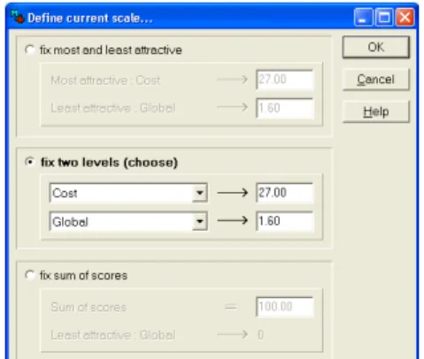
We started by constructing a judgment matrix in the MACBETH that produces as result the weights found by Hokkanen and Salminen. In order to perform that, we set, in the software M-MACBETH, the limit values of the inputs as shown in Figure 1.
Figure 2 illustrates the inputs judgment matrix that was able to produce the desired weights. With the intention of normalizing the outcomes, we generated a MACBETH transformed scale by defining the current scale to have the sum of scores 100. The result, shown in Figure 3, displays the new scale and the bounds that these weights can reach without disagreeing to the judgment matrix. For example: the new value of the criterion Cost is 52.02 and it can vary from 41.43 to 99.87. The same practice was done in relation to the outputs.
resultant weights of the Hokkanen and Salminen’s work, i.e., instead of constructing a matrix by interviewing the DMs and then have the weights as outcomes, we started with the weights and then constructed a matrix that resulted in these weights.
Table 2 – Normalized data of Hokkanen and Salminen’s paper.
INPUTS OUTPUTS
Cost Global Health Acidif. Surface Feasibility Employees Resource 1 0.8945 1.0657 1.2419 0.9874 1.3701 0.7120 0.9112 0.5107 2 1.0717 1.0395 1.1726 0.9874 1.3947 0.5696 1.1716 0.8670 3 1.2435 0.9267 1.3663 1.0140 1.2147 0.5696 1.5621 1.4610 4 0.8031 1.0794 0.8382 0.9883 0.9059 1.2816 0.6509 0.5107 5 0.9626 1.0264 0.6628 0.9883 0.8262 0.9968 0.9112 0.8670 6 1.1372 0.9075 1.0197 1.0173 0.7853 0.9256 1.1716 1.4941 7 0.7908 1.0817 0.8116 0.9883 0.8793 1.2816 0.6509 0.5107 8 0.9299 1.0263 0.6403 0.9883 0.8037 0.9968 0.9112 0.8670 9 1.1426 0.8997 1.0217 1.0198 0.7628 0.9256 1.4320 1.5338 10 0.7895 1.0828 0.7607 0.9883 0.8282 1.2816 0.5858 0.5107 11 0.9381 1.0264 0.5955 0.9883 0.7566 0.9968 0.8462 0.8670 12 1.1426 0.8973 1.0176 1.0206 0.7382 0.9256 1.1065 1.5602 13 0.8113 1.0808 1.0197 0.9883 1.1002 1.2816 0.7811 0.5107 14 0.9667 1.0277 0.8198 0.9883 1.0000 0.9968 1.1065 0.8670 15 1.1576 0.9143 1.3215 1.0173 1.1002 0.9256 1.3018 1.4941 16 0.8236 1.0808 1.0197 0.9883 1.1002 1.2816 0.7811 0.5107 17 1.0035 1.0277 0.8198 0.9883 1.0000 0.9968 1.1065 0.8670 18 1.1876 0.9143 1.3215 1.0173 1.1002 0.9256 1.3018 1.4941 19 0.7895 1.0966 1.0095 0.9899 1.1411 1.2816 0.4556 0.5107 20 0.9476 1.0354 0.8647 0.9916 1.0941 0.8544 1.1716 0.8670 21 1.1276 0.8816 1.3276 1.0264 1.0491 0.9968 1.0414 1.6594 22 1.3390 0.8816 1.3276 1.0281 1.0491 0.9968 1.0414 1.6594
The MACBETH outcomes (bounds divided by 100) for all the inputs and outputs criteria are listed in Table 3. We normalized the MACBETH results (fixed the sum in 100 and then divided the results by 100) in order to allow the outcomes to be used as lower and upper bounds in the Virtual Weights Restrictions approach and to keep the decimal place precision in four digits (the MACBETH standard is two digits).
Table 3 – Upper and lower limits of weights.
Criteria Upper Limit Lower Limit
Cost 0.9987 0.4143
Global Effects 0.0752 0.0002 Health Effects 0.2224 0.1756 Acidificative Releases 0.1600 0.0447 INPUTS
Surface Water Releases 0.1827 0.1317 Technical Feasibility 0.9997 0.4244
Employees 0.4561 0.1390
OUTPUTS
Observe that the upper bound of the criterion Surface is greater than the lower bound of the criterion Health. This fact also occurs with the following pairs of criteria: {(Surface, Acidificative), (Acidificative, Global), (Feasibility, Employee), (Employee, Recovery)}. This situation can lead to a DEA solution that contradicts the MACBETH rank of preference. In order to avoid this, we are going to add some constraints to the Virtual Weights Restrictions DEA model:
*
*
(Health, Surface), (Acidificative, Global), , ( , )
(Surface, Acidificative) (Feasibility, Employees), , ( , )
(Employees, Recovery) i io j jo
i io j jo
v x v x i j I
u y u y i j O
⎧ ⎫ ≥ ∈ = ⎨ ⎬ ⎩ ⎭ ⎧ ⎫ ≥ ∈ = ⎨ ⎬ ⎩ ⎭ (10)
The next step was to run the Virtual Weights Restrictions DEA model augmented by restrictions (10). We named this formulation as Multicriteria DEA model:
1 1 1 1 1 1 1 1
. . : 1
0 , 1, 2, ... ,
. 0 , 1, 2, ... ,
. 0 , 1, 2, ... ,
. 0 , 1, 2, ... ,
. 0 , 1, 2, . s
o r ro r m
i io i
s m
r rj i ij
r i
s k ko k r ro
r s k ko k r ro
r m k ko k i io
i m k ko k i io
i
Max u y
S T v x
u y v x j n
u y UO u y k s
u y LO u y k s
v x UI v x k m
v x LI v x k
θ = = = = = = = = = = − ≤ = − ≤ = − ≥ = − ≤ = − ≥ =
∑
∑
∑
∑
∑
∑
∑
∑
* * .. , , ( , ) , ( , ) , 0 , , i io j jo i io j jo i rm
v x v x i j I
u y u y i j O
v u i r
≥ ∈
≥ ∈
≥ ∀
(11)
where LOk and UOk are, respectively, the lower and upper limits of output k; LIk and k
UI are, respectively, the lower and upper limits of input k; I* and O* are the sets of inputs and outputs, respectively, in which the lower and upper bounds do not obey the MACBETH preference rank.
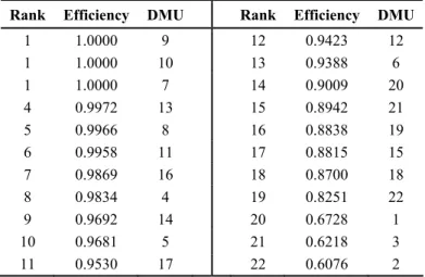
Table 4 – Multicriteria DEA Efficiency.
Rank Efficiency DMU Rank Efficiency DMU
1 1.0000 9 12 0.9423 12
1 1.0000 10 13 0.9388 6
1 1.0000 7 14 0.9009 20
4 0.9972 13 15 0.8942 21
5 0.9966 8 16 0.8838 19
6 0.9958 11 17 0.8815 15
7 0.9869 16 18 0.8700 18
8 0.9834 4 19 0.8251 22
9 0.9692 14 20 0.6728 1
10 0.9681 5 21 0.6218 3
11 0.9530 17 22 0.6076 2
6. Multicriteria DEA Model Results’ Analysis
Salminen et al. (1998) studied three widely used decision-aids Multicriteria models: the ELECTRE III, the SMART and the PROMETHEE I and II. In Table 4 of their paper, they ranked, with the above three models, the same data we used in our numerical example. As our Multicriteria DEA model indicated three DMUs as efficient, we are going to compare them to the three first DMUs ranked by the work of Salminen et al. (1998). This comparison is shown in Table 5.
Table 5 – Rank comparison of several methodologies.
Rank Multicriteria
DEA Model
ELECTRE
III SMART PROM I PROM II
1 9, 10, 7 9 10 10, 7, 4 10
2 6, 11 7 7
3 4 4
Observe that the first DMU ranked by the ELECTRE III and the top two DMUs ranked by the SMART and by the PROMETHEE I and II are the ones our methodology points as efficient. Another aspect that deserves attention is that the bottom four DMUs ranked by all decision-aid Multicriteria methodologies and by the Multicriteria DEA model are exactly the same.
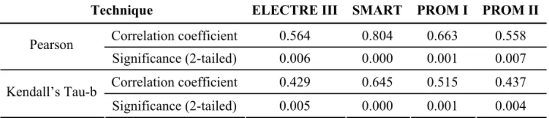
Table 6 – Correlations among the Multicriteria DEA model and traditional Multicriteria methodologies.
Technique ELECTRE III SMART PROM I PROM II
Correlation coefficient 0.564 0.804 0.663 0.558 Pearson
Significance (2-tailed) 0.006 0.000 0.001 0.007 Correlation coefficient 0.429 0.645 0.515 0.437 Kendall’s Tau-b
Significance (2-tailed) 0.005 0.000 0.001 0.004
We made another numerical study with the data presented by Olson (2001). In his work he used the SMART, the SMARTER (centroid approach), the PROMETHEE I (type 6 criterion – Gaussian distribution based on the standard deviation) and the PROMETHEE II to analyze the data of various seasons of American major league professional baseball. The resultant rank of Olson’s paper was compared with the outcomes of the Multicriteria DEA model. We obtained total agreement in all the eight positions of these ranks.
Our numerical studies showed that the DEA characteristic of choosing the best weight for each input/output emulates, in some way, the different preference modeling structure of several Multicriteria models.
As seen in the last two sections, the main advantage of our proposal is:
• The DM does not have to establish weights directly (job that is known to be very difficult) in order to apply a Multicriteria method;
• The DM does not have to blindly accept the outcomes of DEA “black box”.
In other words, the DM can have the best of two worlds: DEA’s needless of setting up weights and MACBETH first steps’ ease of use (the achievement of a pre-cardinal scale).
7. Conclusions
We proposed the utilization of the MACBETH methodology to define the bounds of the weights for the Multicriteria DEA model. The outcomes of our proposal were compared with traditional Multicriteria decision-aids methodologies. This comparison demonstrated evidences of significant correlation among our methodology and the traditional ones. Besides, the Multicriteria DEA model was able to join the most significant outcomes of three traditional Multicriteria decision-aid methodologies in one unique outcome, as seen in last section. This result elects our algorithm as a good approach to generate a wide overview of Multicriteria decision-aid methodologies results.
In our numerical example, we generated a judgment matrix which had as outcomes the weights found in the Hokkanen and Salminen’s paper. In real world applications, we usually do not have these weights clearly defined by the DM(s). The obtainment of these weights has demonstrated to be a thorny issue. This fact justifies the use of MACBETH, since this methodology has proven to be an excellent tool for acquiring the weights.
the problem. Unfortunately, the incorporation of the DM’s preference into DEA models seems more acceptable by the managers’ community. We provided one methodology that does it.
On the other hand, using Multicriteria methodologies can be seen as very difficult by some DM. Our proposal used only the initial steps of a well-known and respected Multicriteria model (MACBETH), facilitating, this way, the DM job.
For future works, we should test the Multicriteria DEA model in further real world problems and compare its results with different decision-aid Multicriteria methodologies.
References
(1) Allen, R.; Athanassopoulos, A.D.; Dyson, R.G. & Thanassoulis, E. (1997). Weights Restrictions and Value Judgments in Data Envelopment Analysis: Evolution, Development and Future Directions. Annals of Operations Research, 73, 13-34.
(2) Bana e Costa, C.A.; De Corte, J.–M. & Vansnick, J.C. (2003). MACBETH. LSE OR Working Paper 03.56. London School of Economics, UK.
(3) Charnes, A.; Cooper, W.W. & Rhodes, E. (1978). Measuring the Efficiency of Decision Making Units. European Journal of Operational Research, 2, 429-444.
(4) Estellita Lins, M.P.; Moreira da Silva, A.C. & Lovell, C.A.K. (2007). Avoiding infeasibility in DEA models with weight restrictions. European Journal of Operational Research, 181, 956-966.
(5) Hokkanen, J. & Salminen, P. (1997). Choosing a Solid Waste Management System Using Multicriteria Decision Analysis. European Journal of Operational Research, 98, 19-36. (6) Liu, C.C. (2003). Simulating Weights Restrictions in Data Envelopment Analysis by
the Subjective and Objective Integrated Approach. Web Journal of Chinese Management Review, 6(1), 68-78.
(7) Olson, D.L. (2001). Comparison of Three Multicriteria Methods to Predict Known Outcomes. European Journal of Operational Research, 130, 576-587.
(8) Saaty, T.L. (1980). The Analytic Hierarchy Process. McGraw-Hill.
(9) Salminen, P.; Hokkanen, J. & Lahdelma, R. (1998). Comparing Multicriteria Methods in the Context of Environmental Problems. European Journal of Operational Research, 104, 485-496.
(10) Shang, J. & Sueyoshi, T. (1995). A Unified Framework for the Selection of a Flexible Manufacturing System. European Journal of Operational Research, 85, 297-315. (11) Sinuany-Stern, Z.; Mehrez, A. & Hada, Y. (2000). An AHP/DEA Methodology for Ranking
Decision Making Units. International Transactions in Operations Research, 7, 109-124. (12) Soares de Mello, J.C.C.B.; Lins, M.P.E.; Soares de Mello, M.H.C.S. & Gomes, E.G.
(2002). Evaluating the performance of calculus using operational research tools.
European Journal of Engineering Education, 27(2), 209-218.
(13) Takamura, Y. & Tone, K. (2003). A Comparative Site Evaluation Study for Relocating Japanese Government Agencies Out of Tokyo. Socio-Economic Planning Sciences, 37, 85-102.
(15) Thompson, R.G.; Singleton, F.D.; Thrall, R.M. & Smith, B.A. (1986). Comparative Site Evaluations for Locating a High-Energy Physics Lab in Texas. Interfaces, 16, 35-49. (16) Wong, Y.-H.B. & Beasley, J.E. (1990). Restricting Weight Flexibility in Data
Envelopment Analysis. Journal of the Operational Research Society, 41(9), 829-835.
Appendices
Figure 1 – Defining current scale in the M-MACBETH software.
Figure 2 – Inputs Judgment Matrix.