Pesqui. Oper. vol.36 número3

(1)

doi: 10.1590/0101-7438.2016.036.03.0547

THE COMPOSED ZERO TRUNCATED LINDLEY-POISSON DISTRIBUTION

Ana Paula Jorge do Espirito Santo

1*

_{and Josmar Mazucheli}

2

Received January 23, 2015 / Accepted October 20, 2016

ABSTRACT.In this paper, a new compounding distribution, named zero truncated Lindley-Poisson distri-bution is introduced. The probability density function, cumulative distridistri-bution function, survival function, failure rate function and quantiles expressions of it are provided. The parameters estimatives were obtained by six methods: maximum likelihood (MLE), ordinary least-squares (OLS), weighted least-squares (WLS), maximum product of spacings (MPS), Cram´er-von-Mises (CM) and Anderson-Darling (AD), and intensive simulation studies are conducted to evaluate the performance of parameter estimation. Some generaliza-tions are also proposed. Application in a real data set is given and shows that the composed zero truncated Lindley-Poisson distribution provides better fit than the Lindley distribution and three of its generalizations. The paper is motivated by application in real data set and we hope this model may be able to attract wider applicability in survival and reliability.

Keywords: compounding, estimation methods, Lindley distribution, survival analysis, zero truncated Poisson distribution.

1 INTRODUCTION

The one parameter Lindley distribution was introduced by Lindley (see, Lindley 1958 and 1965) as a new distribution useful to analyze lifetime data, especially in stress-strength reliability mod-eling. Suppose thatT1, . . . ,TMare independent and identically distributed random variables fol-lowing the one parameter Lindley distribution with probability density function and distribution function written, respectively, as:

f1(t |θ ) = θ2

(θ+1)(1+t)e

−θt ₍₁₎

F1(t |θ ) = 1−

1+ θt θ+1

e−θt (2)

wheret >0 andθ >0.

*Corresponding author.

(2)

For a random variable with the one parameter Lindley distribution, the probability density func-tion,(1), is unimodal for 0< θ <1 and decreasing whenθ >1 (see Fig. 1-a). The hazard rate function is an increasing function int andθ(see Fig. 1-b) and given by:

h1(t|θ )=

θ2(1+t)

(1+θ+θt). (3)

0 5 10 15 20

0.0

0.2

0.4

0.6

0.8

t

f(t)

θ= 0.2 θ= 0.5 θ= 1.0 θ= 1.5

(a)

0 5 10 15 20

0.0

0.5

1.0

1.5

t

f(t)

θ= 0.2 θ= 0.5 θ= 1.0 θ= 1.5

(b)

(3)

in the competing risks scenario was considered in Mazucheli & Achcar (2011). The exponen-tial Poisson Lindley distribution was presented in Barreto-Souza & Bakouch (2013). Ghitany et al. (2013) introduced the power Lindley distribution. Ali (2015) investigated various proper-ties of the weighted Lindley distribution which main focus was the Bayesian analysis. A new four-parameter class of generalized Lindley distribution called the beta-generalized Lindley dis-tribution is proposed by Oluyede & Yang (2015).

Aim to offers more flexible distributions for modeling lifetime data set, in this paper, is proposed an extension of the Lindley distribution. We consider thatTj, j =1, . . .,Mis a random sample from the one parameter Lindley distribution and that our variable of interest is defined as:

(i) Y =min(T1, . . .,TM) and (ii) Y =max(T1, . . .,TM)

representing, respectively, the first and the last failure time of a certain device subject to the presence of an unknown number M of causes of failures. Furthermore, we consider that M has a zero truncated Poisson distribution, M ∼ PoissonT runc(λ), λ > 0, and that Tj,

j = 1, . . .,M, and M are independent random variables, leading to the composed zero trun-cated Lindley-Poisson distribution. The process of composition using the zero truntrun-cated Pois-son distribution has been fairly used in the literature. In Kus¸ (2007) was considered the zero truncated Exponential-Poisson distribution in the competing risks scenario. Hemmati et al. (2011) developed the zero truncated Weibull-Poisson distribution. Also in 2011, the same distri-bution was studied by Risti´c & Nadarajah (2012) and Lu & Shi (2012). The zero truncated Exponential-Poisson distribution in the complementary risks scenario was introduced by Rezaei & Tahmasbi (2012).

The paper is organized as follows: in Section 2 the zero truncated Lindley-Poisson distribution is formulated. In Section 3 six estimation methods are presented. A simulation study is introduced in Section 4. The Section 5 brings a real data application. And finally, conclusions are presented in Section 6.

2 MODEL FORMULATION

In the theory of competing risks and complementary risks the number of risk factors (or causes) that may lead to the event of interest, is known and denoted asM. However, in models of dis-tributions composition is assumed thatMis unknown. Therefore, there is a numberM of latent risk factors competing to cause the event of interest. In what follows, let us consider the situa-tion where an individual or unit is exposed toM possible causes of death or failure, such that the exact cause is fully known (David & Moeschberger, 1978). The model for lifetime in the presence of suchcompeting risks structure or complementary risks structure is known as model of composition distributions. IfTj, j = 1, . . . ,M denote the latent failure times of a individ-ual subject to M risks, which are independent of M, what is observed is the time to failure Y = min(T1, . . . ,TM). Given M = m, under the assumption that the latent failure times Tj,

(4)

function(2), the probability density function and the cumulative distribution function are written, respectively, as:

f(y| M =m, θ ) = mθ

2₍₁₊_y₎_e−θy θ+1

1+ θy θ+1

e−θy

m−1

, (4)

F(y|θ ,M =m) = 1−

1+ θy θ+1

e−θy

m

. (5)

It is important to note that (4) and (5) are uniquely determined by the distribution function of the minimum, that is,P(Y ≤ y)=1−[1−F1(y|θ )]m, (Arnold et al., 2008).

Now, assuming the number of causes of death or failure,M, is a zero truncated Poisson random variable with probability mass function given by:

P(M =m)= λ

m_e−λ

m!(1−e−λ₎, (6)

wherem=1,2, . . .andλ >0, Rezaei & Tahmasbi (2012).

The marginal probability density function, fmin(y|θ , λ), the marginal cumulative distribu-tion funcdistribu-tion, Fmin(y|θ , λ), and the marginal hazard rate function, hmin(y|θ , λ) of Y = min(T1, . . .,TM)are given, respectively, by:

fmin(y|θ , λ) =

λθ2(1+y)e−

θy+λ1−1+_θθy₊₁e−θy

(θ+1)(1−e−λ₎ , (7)

Fmin(y|θ , λ) =

1−e−λ

1−1+_θθy₊₁e−θy

1−e−λ , (8)

hmin(y|θ , λ) =

λθ2(1+y)e−

θy+λ

(θ+1)

e−λ

−e−λ

, (9)

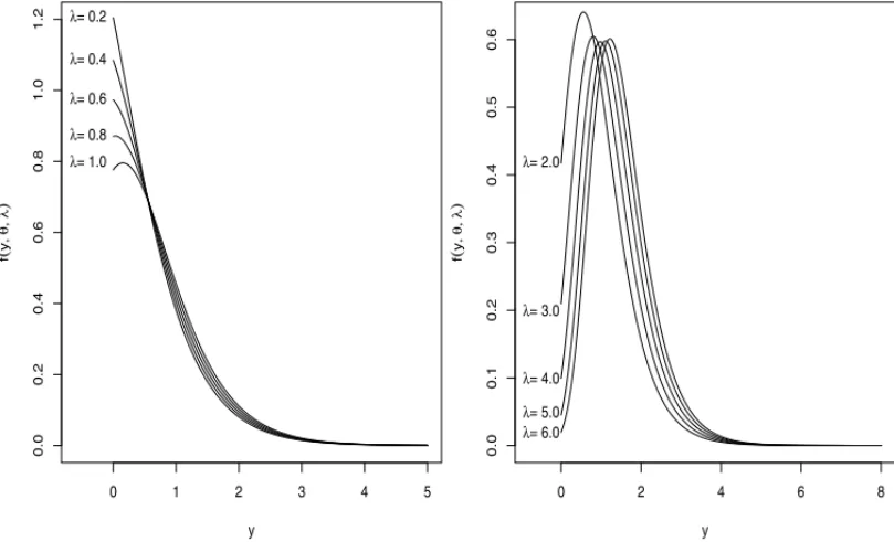
whereθ >0, λ >0 andy>0, which defines the zero truncated Lindley-Poisson distribution in the competing risks scenario. Taking theλ=0 we have the one parameter Lindley distribution as a particular case. Note that fmin(0|θ , λ) = λθ

2

(θ+1)(1−e−λ₎ and fmin(∞ |θ , λ) =0. For all

θ > 0 andλ > 0, the probability density function, (7), is decreasing or unimodal (see Fig. 2). For values of λclose to 1, the curve resembles the one parameter Lindley distribution, while whenλ−→0 the curve tends to be symmetric.

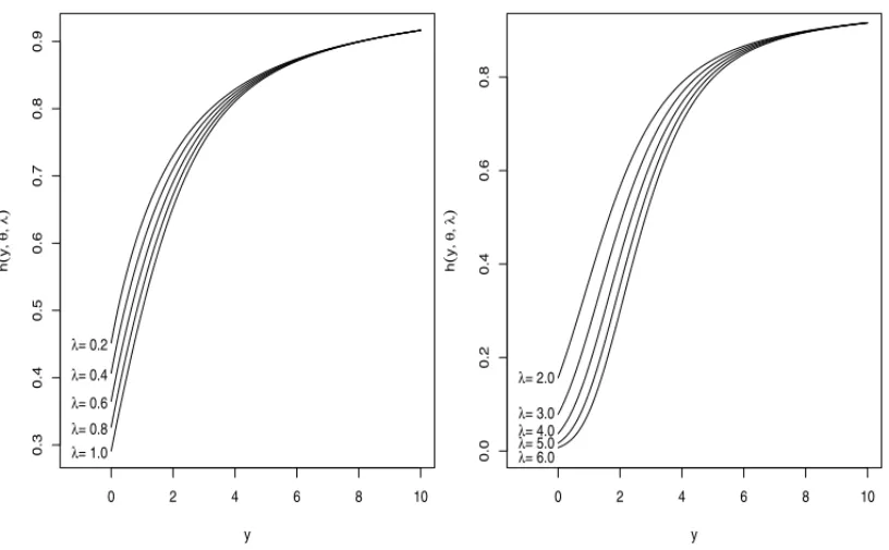
The hazard rate, (9), is increasing, increasing-decreasing-increasing and decreasing (see Fig. 3). Is easy to see thathmin(0|θ , λ)= fmin(0|θ , λ)= λθ

2

(θ+1)(1−e−λ₎andhmin(∞ |θ , λ)=θ.

(5)

0 2 4 6 8 10

0.00

0.05

0.10

0.15

0.20

0.25

y

f

(

y

, θ, λ

)

λ= 1.0 λ= 0.8 λ= 0.6 λ= 0.4 λ= 0.2

0 2 4 6 8 10

0.0

0.2

0.4

0.6

0.8

1.0

y

f

(

y

, θ, λ

)

λ= 6.0

λ= 5.0

λ= 4.0

λ= 3.0

λ= 2.0

Figure 2–The zero truncated Lindley-Poisson probability density function for different values of theλ

andθ=0.5 ifY =min(T1, . . . ,TM).

0 2 4 6 8 10

0.5

0.6

0.7

0.8

0.9

y

h

(

y

, θ, λ

)

λ= 0.2 λ= 0.4 λ= 0.6 λ= 0.8 λ= 1.0

0 2 4 6 8 10

1.0

1.5

2.0

2.5

3.0

3.5

y

h

(

y

, θ, λ

)

λ= 3.0 λ= 4.0 λ= 5.0 λ= 6.0 λ= 7.0

Figure 3–The zero truncated Lindley-Poisson hazard rate function for different values of theλandθ=2.0

(6)

0 1 2 3 4 5

0.0

0.2

0.4

0.6

0.8

1.0

1.2

y

f

(

y

, θ, λ

)

λ= 1.0 λ= 0.8 λ= 0.6 λ= 0.4 λ= 0.2

0 2 4 6 8

0.0

0.1

0.2

0.3

0.4

0.5

0.6

y

f

(

y

, θ, λ

)

λ= 6.0 λ= 5.0 λ= 4.0 λ= 3.0 λ= 2.0

Figure 4–The zero truncated Lindley-Poisson probability density function for different values of theλ

andθ=2.0 ifY=max(T1, . . . ,TM).

fmax(y|θ , λ), the cumulative distribution function,Fmax(y|θ , λ), and the hazard rate func-tion,hmax(y|θ , λ), are given, respectively, by:

fmax(y|θ , λ) =

λθ2(1+y)e−

θy+λ

1+₁θy₊_θe−θy

(1+θ )(1−e−λ₎ , (10)

Fmax(y|θ , λ) = e−λ

1+₁θ₊y_θe−θy

−e−λ

1−e−λ , (11)

hmax(y|θ , λ) =

λθ2(1+y)e−

θy+λ1+₁θy₊_θe−θy

(1+θ )

1−e−λ

1+₁θy₊_θe−θy . (12)

whereθ >0, λ >0 andy>0. Note that fmax(0|θ , λ)= λθ

2_e−λ

(θ+1)(1−e−λ₎ and fmax(∞ |θ , λ)=0. For allθ >0 andλ >0 the

(7)

For allθ > 0 andλ > 0, the hazard rate function, (12), is increasing (see Fig. 5). Is easy to see thathmax(0|θ , λ) = fmax(0|θ , λ) = λθ

2_e−λ

(θ+1)(1−e−λ₎ andhmax(∞ |θ , λ) = θ. Note that

hmin(∞ |θ , λ)=hmax(∞ |θ , λ)=θ.

0 2 4 6 8 10

0.3

0.4

0.5

0.6

0.7

0.8

0.9

y

h

(

y

, θ, λ

)

λ= 0.2

λ= 0.4

λ= 0.6

λ= 0.8 λ= 1.0

0 2 4 6 8 10

0.0

0.2

0.4

0.6

0.8

y

h

(

y

, θ, λ

)

λ= 2.0

λ= 3.0 λ= 4.0 λ= 5.0 λ= 6.0

Figure 5–The zero truncated Lindley-Poisson hazard rate function for different values of theλandθ=2.0

ifY =max(T₁, . . . ,TM).

Glaser (1980) and Chechile (2003) studied the hazard rate function behavior by theη (y) =

−f´′(y|θ ,λ)

f(y|θ ,λ) function and its derivativeη′(y). Because of the complexity of such studies, this work only presents the functionsη (y)andη′(y). Considering the hazard rate functions (9) and (12), we have:

η (y)_min = e

−θy_θ2_{λ (}_y₊₁₎2₊_(θ₊₁₎_eθy_(θ₊_θ_y₋₁₎

(θ+1) (y+1) , (13)

η (y)max = −

e−θyθ2λ (y+1)2−(θ+1)eθy(θ+θy−1)

(θ +1) (y+1) . (14)

and its first derivatives are:

η′(y)_min = e

−θy_(θ₊₁₎_eθy₋_θ2_{λ (}_y₊₁₎2_(θ ₊_θ_y₋₁₎

(θ+1) (y+1)2 ,

η′(y)_max = −e

−θy_(θ₊₁₎_eθy₊_θ2_{λ (}_y₊₁₎2_(θ₊_θ_y₋₁₎

(8)

Therefore, the hazard rate function behavior properties of the zero truncated Lindley-Poisson distribution follows from the results in Glaser (1980) and Chechile (2003).

2.1 Quantile function

The quantile function of the zero truncated Lindley-Poisson distribution is given by:

F−1(u)= −1−1

θ −

1 θW−1

−(θ +1) eθ+1

lnu+eλ−ueλ λ

if Y = min(T1, . . .,TM), where 0 < u < 1 and W−1(·)denotes the negative branch of the Lambert W function (i.e., the solution of the equationW(z)eW(z)=z) because(1+θ+θy) >1 and−(θ_eθ++11)

lnu+eλ₋_ueλ

λ ∈

−1_e,0. And, the quantile function of the zero truncated Lindley-Poisson distribution is given by:

F−1(u)= −1−1

θ −

1 θW−1

(θ+1)

eθ+1

ln1+ueλ−u−λ λ

if Y = max(T1, . . .,TM), where 0 < u < 1 and W−1(·)denotes the negative branch of the Lambert W function because (1+θ+θy) > 1 and (θ+1)

eθ+1

ln1+ueλ₋_u₋_λ

λ ∈

−1_e,0(Jodr´a, 2010; Ghitany et al., 2012).

Our approach may be generalized in some different ways, for instance, it is important to note that for any probability density function f1(y|θ),θ =θ1, . . . , θp

, and M ∼ PoissonT runc(λ) as the discrete distribution, the general marginal probability density function can be written as:

f(y|θ , λ) = λe

−λ_f

1(y|θ)

1−e−λ

∞

m=1

λFp(y|θ) m−1

(m−1)! = λf1(y|θ)e

−λFp(y|θ)

1−e−λ , (15)

whereFp(y|θ)=F1(y|θ)whenY =min(T1, . . .,TM)andFp(y|θ)=1−F1(y|θ)when Y =max(T1, . . .,TM).

From (15), the cumulative distribution, survival and hazard functions forY =min(T1, . . .,TM) andY =max(T1, . . .,TM)can be generically written as:

Fmin(y|θ, λ)=1−e

−λF₁(y|θ)

1−e−λ , Fmax(y|θ, λ)=

e−λS1(y|θ)−e−λ 1−e−λ ,

Smin(y|θ, λ)= e

−λF₁(y|θ₎

−e−λ

1−e−λ , Smax(y|θ, λ)=

1−e−λS1(y|θ)

1−e−λ ,

hmin(y|θ, λ)= λf1(y|

θ₎e−λF₁(y|θ)

e−λF1(y|θ)₋_e−λ , hmax(y|θ, λ)=

λf1(y|θ)e−λS1(y|θ)

1−e−λF1(y|θ) .

3 ESTIMATION METHODS

(9)

andθare unknown. This is also considered in the simulation study presented in Section 4. Note that the methods were presented for a general baseline function f1(y|θ ).

3.1 Maximum Likelihood

Lety =(y1, . . . ,yn)be a random sample ofnsize from the distribution obtained by the com-position of distributions with parametersλandθ, the likelihood and log-likelihood function are, respectively:

L(θ , λ|y)=

n

i=1

f(yi|θ , λ)=

λnn_i₌₁ f1(yi|θ )e−λ

n

i=1Fp(yi|θ )

1−e−λn , (16)

l(θ , λ|y)=nlogλ−nlog1−e−λ+

n

i=1

log f1(yi|θ )−λ n

i=1

Fp(yi|θ ) , (17) where:

i) Fp(yi |θ )=F1(yi |θ )ifY =min(T1, . . .,TM) ii) Fp(yi |θ )=1−F1(yi |θ )ifY =max(T1, . . .,TM).

The maximum likelihood estimates ofθandλ,θM L E andλM L E respectively, can be obtained numerically by maximizing the log-likelihood function(17). In this case, the log-likelihood function is maximized by solving numerically _∂θ∂ l(θ ,λ|y) = 0 and _∂λ∂ l(θ ,λ|y) = 0 inθ andλ, respectively, where:

∂

∂θl(θ ,λ|y) = n

i=1

f₁′(yi|θ )

f1(yi|θ )

−λ n

i=1

F_p′(yi|θ ) , (18)

∂

∂λl(θ ,λ|y) = n

λ−

ne−λ

1−e−λ−

n

i=1

Fp(yi|θ ) , (19)

where f₁′(yi |θ )=_∂θ∂ f1(yi |θ )andFp′(yi |θ )=_∂θ∂ Fp(yi |θ ).

3.2 Ordinary Least-Squares

Lety1:n<y2:n· · ·<yn:nbe the order statistics of a random sample ofnsize from a distribution with cumulative distribution functionF(y). It’s well known that:

EFy(i:n)

= i

n+1 and V ar

Ft(i:n)

= i(n−i+1)

(n+1)2(n+2). (20) For the distribution obtained by the composition process, the least square estimatesθO L S and λO L Sof the parametersθandλ, respectively, are obtained by minimizing the function:

n

i=1

1−e−λF1(yi:n|θ )

1−e−λ − i n+1

2

(10)

whenY =min(T1, . . .,TM), and minimizing n

i=1

e−λS1(yi:n|θ )₋_e−λ

1−e−λ − i n+1

2

, (22)

whenY =max(T1, . . .,TM).

Therefore, ifY =min(T1, . . .,TM), these estimates can also be obtained by solving the nonlin-ear equations:

n

i=1

1−e−λ − i n+1

1(yi:n|θ , λ) = 0 (23)

n

i=1

1−e−λ − i n+1

2(yi:n|θ , λ) = 0 (24)

where:

1(yi:n|θ , λ) =

λ_∂θ∂ F1(yi:n|θ )

e−λF1(yi:n|θ )

1−e−λ (25)

2(yi:n|θ , λ) =

F1(yi:n|θ )e−λF1(yi:n|θ )

1−e−λ −

1−e−λF1(yi:n|θ )_e−λ

1−e−λ2 (26)

But, if Y = max(T1, . . .,TM), these estimates can also be obtained by solving the nonlinear equations:

n

i=1

1−e−λ − i n+1

1(yi:n|θ , λ) = 0 (27)

n

i=1

1−e−λ − i n+1

2(yi:n|θ , λ) = 0 (28)

where:

1(yi:n|θ , λ) = −

λ_∂θ∂ S1(yi:n|θ )

e−λS1(yi:n|θ )

1−e−λ (29)

2(yi:n|θ , λ) =

−S1(yi:n|θ )e−λS1(yi:n|θ )

1−e−λ −

e−λS1(yi:n|θ )₋_e−λ_e−λ

1−e−λ2 (30)

(11)

3.3 Weighted Least-Squares

The weighted least-squares estimatesθW L S andλW L S of the parameters θ andλ, respectively, are obtained by minimizing the function:

n

i=1 wi

1−e−λF1(y|θ )

1−e−λ − i n+1

2

, (31)

ifY =min(T1, . . .,TM), and minimizing n

i=1 wi

e−λS1(y|θ )₋_e−λ

1−e−λ − i n+1

2

, (32)

ifY =max(T1, . . .,TM).

The correction factorwiis given by:

wi = 1 VF(y(i:n))

= (n+1)

2₍_n₊₂₎

i(n −i+1) . (33)

Therefore, ifY =min(T1, . . .,TM), these estimates can also be obtained by solving the nonlin-ear equations:

n

i=1 1 i(n−i+1)

1−e−λF1(y|θ )

1−e−λ − i n+1

1(yi:n|θ , λ) = 0 (34)

n

i=1 1 i(n−i+1)

1−e−λF1(y|θ )

1−e−λ − i n+1

2(yi:n|θ , λ) = 0 (35)

where1(yi:n|θ , λ)and2(yi:n|θ , α)are given by (25) and (26), respectively.

Thus, ifY =max(T1, . . .,TM), these estimates can also be obtained by solving the nonlinear equations:

n

i=1 1 i(n−i+1)

1−e−λ − i n+1

1(yi:n|θ , λ) = 0 (36)

n

i=1 1 i(n−i+1)

1−e−λ − i n+1

2(yi:n|θ , λ) = 0 (37)

where1(yi:n|θ , λ)and2(yi:n|θ , α)are given by (29) and (30), respectively.

3.4 Maximum Product of Spacings

(12)

measure of information. In what follows, let y1:n < y2:n <· · · < yn:n be an ordered random sample drawn from the general model of composition distribution. Are defined as the uniform spacings of the sample the quantities: D1 = F(y1:n|θ , λ), Dn+1 = 1−F(tn:n|θ , λ) and

Di = F(ti:n|θ , λ)−Ft(i−1):n|θ , λ,i =2, . . . ,n. There are(n+1)spacings of the first order.

Following Cheng & Amin (1983), the maximum product of spacings method consists in finding the values ofθandλwhich maximize the geometric mean of the spacings, the MPS statistics, is given by:

G(θ , λ)=

_n₊₁

i=1 Di

1 n+1

(38)

or, equivalently, its logarithmH =log(G). Considering 0=F(t0:n|θ , λ) <F(y1:n|θ , λ) <

· · ·<F(yn:n|θ , λ) <F

y(n+1):n|θ , λ

=1 the quantitieH =log(G)can be calculated as:

H(θ , λ)= 1 n+1

n+1

i=1

log [Di]. (39)

The estimates forθandλcan be found solving, respectively inθandλ, the nonlinear equations:

∂

∂θH(θ , λ) = n+1

i=1 1 Di

_∂

∂θ F(yi:n|θ , λ)

=0 (40)

∂

∂αH(θ , λ) = n+1

i=1 1 Di

∂

∂αF(yi:n|θ , λ)

=0 (41)

whereis the first order difference operator.

Cheng & Amin (1983) showed that maximizing H as a method of parameter estimation is as efficient as MLE estimation and the MPS estimators are consistent under more general conditions than the MLE estimators.

Therefore, ifY =min(T1, . . .,TM), the estimatesθˆM P SandλˆM P Scan be obtained by solving the nonlinear equations:

∂

∂θH(θ , λ) = n+1

i=1 1 Di ∂ ∂θ

1−e−λ

=0 (42)

∂

∂λH(θ , λ) = n+1

i=1 1 Di ∂ ∂λ

1−e−λ

(13)

Thus, ifY =max(T1, . . .,TM), the estimatesθˆM P S andλˆM P S can be obtained by solving the nonlinear equations:

∂

∂θH(θ , λ) = n+1

i=1 1 Di

∂ ∂θ

1−e−λ

=0 (44)

∂

∂λH(θ , λ) = n+1

i=1 1 Di

∂ ∂λ

1−e−λ

=0 (45)

3.5 Minimum distance methods

In this subsection we present two estimation methods forθ andλbased on the minimization of the goodness-of-fit statistics. This class of statistics is based on the difference between the estimate of the cumulative distribution function and the empirical distribution function (Luce˜no, 2006).

3.5.1 Cram´er-von-Mises

The Cram´er-von-Mises estimates of the parametersθC M andλC M, respectively, are obtained by minimizing, inθandλ, the function:

C(θ , λ)= 1 12n +

n

i=1

F(yi:n|θ , λ)− 2i−1

2n

2

. (46)

These estimates can also be obtained by solving the nonlinear equations: n

i=1

F(yi:n|θ , λ)− 2i−1

2n

1(yi:n|θ , λ) = 0 (47)

n

i=1

F(yi:n|θ , λ)− 2i−1

2n

2(yi:n|θ , λ) = 0 (48)

where 1(·|θ , λ) and 2(·|θ , λ) are given, respectively, by (25) and (26) if Y = min(T1, . . . ,TM)and, respectively, by (29) and (30) ifY =max(T1, . . . ,TM).

3.5.2 Anderson-Darling

The Anderson-Darling estimates of the parametersθAD andλˆAD, respectively, are obtained by minimizing, with respect toθandλ, the function:

A(θ , λ)= −n−1 n

n

i=1

(2i−1)logF(yi:n|θ , λ)

1−F(yn+1−i:n|θ , λ)

(14)

These estimates can also be obtained by solving the nonlinear equations: n

i=1

(2i−1)

1(yi:n|θ , λ)

F(yi:n|θ , λ)

−1(yn+1−i:n|θ , λ) F(yn+1−i:n|θ , λ)

= 0 (50)

n

i=1

(2i−1)

2(yi:n|θ , λ)

F(yi:n|θ , λ)

−2(yn+1−i:n|θ , λ) F(yn+1−i:n|θ , λ)

= 0 (51)

where 1(·|θ , λ) and 2(·|θ , λ) are given, respectively, by (25) and (26) if Y = min(T1, . . . ,TM)and, respectively, by (29) and (30) ifY =max(T1, . . . ,TM).

4 SIMULATION STUDY

In this section we present results of some numerical experiments to compare the performance of the different estimation methods discussed in the previous section. We have taken sample sizes n = 20,50,100 and 200, θ = 1.0 andλ = 0.5,1.0,2.0,3.0 and 5.0. For each combination (n, θ , λ)we have generated B = 500,000 pseudo random samples from the zero truncated Lindley-Poisson distribution.

The estimates were obtained inOx version 6.20 (Doornik, 2007) usingMaxBFGSfunction in MLE, OLS, WLS, MPS, CM and AD methods. For each estimate we computed the bias, the root mean-squared error, the average absolute difference between the true and estimate distribu-tions funcdistribu-tions and the maximum absolute difference between the true and estimate distribudistribu-tions functions, respectively, as:

Biasθˆ

= 1 B

B

i=1

ˆ θi−θ

, Biasλˆ

= 1 B

B

i=1

ˆ λi−λ

, (52)

R M S Eθˆ =

1 B B

i=1

ˆ θi −θ

2

, R M S Eλˆ=

1 B B

i=1

ˆ λi−λ

2

, (53)

Dabs = 1 B×n

B

i=1 n

j=1

Fyi j|θ , λ

−F

yi j| ˆθ ,λˆ, (54)

Dmax = 1 B

B

i=1 max

j

Fyi j|θ , λ

−F

yi j| ˆθ ,λˆ. (55)

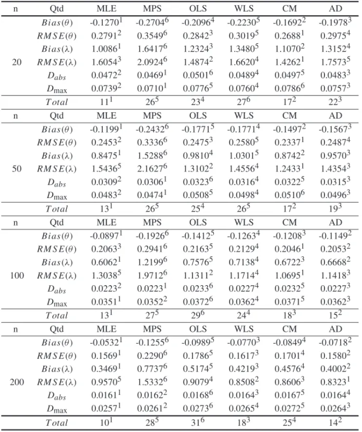
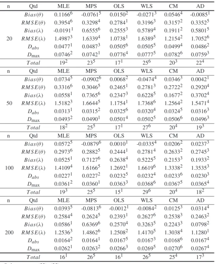
In Tables 1, 2, 3, 4 and 5 we show the calculated values of (52)–(55). The superscript values indicate the rank obtained by each of the methods considered, and thetotalline shows the global rank for each method based on measures (52)–(55).

(15)

Table 1–Simulations results forθ=1.0 andλ=0.5.

n Qtd MLE MPS OLS WLS CM AD

20

Bi as(θ ) -0.12701 -0.27046 -0.20964 -0.22305 -0.16922 -0.19783

RM S E(θ ) 0.27912 0.35496 0.28423 0.30195 0.26881 0.29754

Bi as(λ) 1.00861 1.64176 1.23243 1.34805 1.10702 1.31524

RM S E(λ) 1.60543 2.09246 1.48742 1.66204 1.42621 1.75735

Dabs 0.04722 0.04691 0.05016 0.04894 0.04975 0.04833 Dmax 0.07392 0.07101 0.07765 0.07604 0.07866 0.07573

T otal 111 265 234 276 172 223

50

Bi as(θ ) -0.11991 -0.24326 -0.17715 -0.17714 -0.14972 -0.15673

RM S E(θ ) 0.24532 0.33366 0.24753 0.25805 0.23371 0.24874

Bi as(λ) 0.84751 1.52886 0.98104 1.03015 0.87422 0.95703

RM S E(λ) 1.54365 2.16276 1.31022 1.45564 1.24331 1.43543

Dabs 0.03092 0.03061 0.03236 0.03164 0.03225 0.03153 Dmax 0.04832 0.04741 0.05085 0.04984 0.05106 0.04963

T otal 131 265 254 265 172 193

100

Bi as(θ ) -0.08971 -0.19266 -0.14125 -0.12634 -0.12083 -0.11492

RM S E(θ ) 0.20633 0.29416 0.21635 0.21294 0.20461 0.20532

Bi as(λ) 0.60621 1.21996 0.75765 0.71384 0.67223 0.66682

RM S E(λ) 1.30385 1.97126 1.13112 1.17144 1.06951 1.14183

Dabs 0.02232 0.02231 0.02336 0.02274 0.02325 0.02273 Dmax 0.03511 0.03522 0.03726 0.03624 0.03715 0.03623

T otal 131 275 296 244 183 152

200

Bi as(θ ) -0.05321 -0.12556 -0.09895 -0.07703 -0.08494 -0.07182

RM S E(θ ) 0.15691 0.22906 0.17865 0.16173 0.17014 0.15802

Bi as(λ) 0.34691 0.77376 0.51745 0.42193 0.45764 0.40022

RM S E(λ) 0.95705 1.53326 0.90794 0.85082 0.86063 0.83231

Dabs 0.01611 0.01622 0.01686 0.01643 0.01675 0.01644 Dmax 0.02571 0.02612 0.02736 0.02654 0.02725 0.02643

T otal 101 285 316 183 254 142

Qtd: measures (52)–(55)

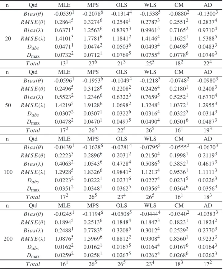
In Tables 6, 7, 8, 9 and 10 we show the calculated values of (52)–(55). The superscript values indicate the rank obtained by each of the methods considered, and thetotalline shows the global rank for each method based on measures (52)–(55).

(16)

20

Bi as(θ ) -0.05391 -0.20786 -0.13144 -0.15385 -0.08802 -0.13003

RM S E(θ ) 0.28645 0.32746 0.25491 0.27873 0.25512 0.28374

Bi as(λ) 0.63711 1.25636 0.83973 0.99615 0.71652 0.97104

RM S E(λ) 1.41013 1.77816 1.18412 1.41464 1.16251 1.53885

Dabs 0.04711 0.04742 0.05036 0.04934 0.04985 0.04833 Dmax 0.07322 0.07121 0.07695 0.07554 0.07786 0.07493

T otal 131 276 213 255 182 224

50

Bi as(θ ) -0.05961 -0.19536 -0.10494 -0.12185 -0.07482 -0.09803

RM S E(θ ) 0.24965 0.31286 0.22082 0.24264 0.21801 0.24083

Bi as(λ) 0.55232 1.23466 0.63223 0.76595 0.52521 0.67704

RM S E(λ) 1.42195 1.91286 1.06982 1.32484 1.03721 1.29553

Dabs 0.03072 0.03071 0.03226 0.03164 0.03225 0.03143 Dmax 0.04782 0.04701 0.04975 0.04904 0.05016 0.04873

T otal 172 265 224 265 161 193

100

Bi as(θ ) -0.04391 -0.16286 -0.07814 -0.07955 -0.05552 -0.06703

RM S E(θ ) 0.22235 0.28966 0.20312 0.21504 0.19981 0.21193

Bi as(λ) 0.40632 1.05436 0.47284 0.50865 0.38521 0.46173

RM S E(λ) 1.29285 1.83266 0.98412 1.12134 0.95361 1.11113

Dabs 0.02232 0.02221 0.02316 0.02274 0.02315 0.02263 Dmax 0.03512 0.03481 0.03625 0.03564 0.03646 0.03563

T otal 172 265 234 265 161 183

200

Bi as(θ ) -0.02451 -0.11946 -0.05085 -0.04444 -0.03402 -0.03833

RM S E(θ ) 0.18945 0.25136 0.18484 0.18473 0.18231 0.18242

Bi as(λ) 0.24881 0.77836 0.32085 0.30124 0.25292 0.27703

RM S E(λ) 1.08765 1.59696 0.88122 0.93084 0.85601 0.92333

Dabs 0.01622 0.01621 0.01675 0.01644 0.01676 0.01643 Dmax 0.02592 0.02581 0.02675 0.02624 0.02686 0.02623

T otal 161 265 265 234 183 172

Lindley-Poisson distribution toY =max(T1, . . . ,TM)to understand why the MLE method was not as good would be very relevant.

(17)

20

Bi as(θ ) 0.11666 -0.07615 0.01502 -0.02713 0.05464 -0.00851

RM S E(θ ) 0.39546 0.32984 0.27841 0.31963 0.31572 0.33525

Bi as(λ) -0.01911 0.65556 0.25553 0.57894 0.19112 0.58015

RM S E(λ) 1.49873 1.63394 1.07381 1.63895 1.21542 1.70526

Dabs 0.04771 0.04873 0.05056 0.05055 0.04994 0.04862 Dmax 0.07462 0.07421 0.07764 0.07775 0.07826 0.07593

T otal 192 235 171 256 203 224

50

Bi as(θ ) 0.07345 -0.09026 0.00682 -0.04744 0.03463 0.00421

RM S E(θ ) 0.33166 0.30465 0.24651 0.27813 0.27222 0.29204

Bi as(λ) 0.05581 0.73656 0.23473 0.62285 0.16772 0.37024

RM S E(λ) 1.51823 1.66445 1.17541 1.73686 1.25642 1.54714

Dabs 0.03131 0.03152 0.03256 0.03204 0.03245 0.03163 Dmax 0.04932 0.04901 0.05014 0.05025 0.05066 0.04963

T otal 182 255 171 276 204 193

100

Bi as(θ ) 0.05725 -0.08796 0.00101 -0.03354 0.02062 0.02373

RM S E(θ ) 0.29736 0.28825 0.24441 0.27814 0.26332 0.27453

Bi as(λ) 0.05251 0.71276 0.26384 0.52255 0.21533 0.19332

RM S E(λ) 1.41094 1.61665 1.26921 1.66196 1.33382 1.35353

Dabs 0.02271 0.02272 0.02325 0.02324 0.02336 0.02303 Dmax 0.03612 0.03601 0.03633 0.03686 0.03675 0.03654

T otal 193 255 151 296 204 182

200

Bi as(θ ) 0.03935 -0.08136 -0.00121 -0.00842 0.01253 0.03144

RM S E(θ ) 0.25844 0.26245 0.23931 0.26276 0.25383 0.24632

Bi as(λ) 0.05861 0.63696 0.25704 0.32635 0.22433 0.07982

RM S E(λ) 1.25363 1.48626 1.25082 1.41705 1.30384 1.12801

Dabs 0.01642 0.01641 0.01675 0.01673 0.01686 0.01674 Dmax 0.02621 0.02632 0.02663 0.02695 0.02706 0.02674

T otal 161 265 161 265 254 173

5 REAL DATA APPLICATION

In this section we fit the zero truncated Lindley-Poisson distribution (LP) to a real data set. For comparison, we also have considered four alternative models: the one parameter Lindley distribution (L) f (y|θ )= ₁θ₊2_θ (1+y)e−θy, the weighted Lindley distribution (WL)

f (y|θ , λ)= θ λ+1

(θ+λ) Ŵ (λ)y

(18)

20

Bi as(θ ) 0.10375 -0.08234 0.04903 -0.03582 0.02261 -0.11516

RM S E(θ ) 0.51686 0.35395 0.31521 0.32662 0.33893 0.34734

Bi as(λ) 0.77984 0.91085 0.04561 0.63623 0.34932 1.28836

RM S E(λ) 4.11806 2.90455 1.55501 2.28613 1.88622 2.78334

Dabs 0.04903 0.05226 0.04965 0.04954 0.04831 0.04892 Dmax 0.07545 0.07776 0.07452 0.07504 0.07441 0.07493

T otal 295 316 132 183 101 254

50

Bi as(θ ) -0.02001 -0.14664 -0.04772 -0.18566 -0.07193 -0.18455

RM S E(θ ) 0.44296 0.33815 0.28931 0.33373 0.30762 0.33464

Bi as(λ) 1.33683 1.34004 0.58801 1.66535 0.81702 1.69556

RM S E(λ) 4.10316 3.00495 1.93321 2.99054 2.13632 2.96613

Dabs 0.03424 0.03566 0.03332 0.03455 0.03301 0.03343 Dmax 0.05354 0.05436 0.05091 0.05385 0.05132 0.05233

T otal 243 306 81 285 122 243

100

Bi as(θ ) -0.08251 -0.17674 -0.13672 -0.26566 -0.16123 -0.23585

RM S E(θ ) 0.40276 0.32753 0.30441 0.35535 0.31952 0.34094

Bi as(λ) 1.41362 1.41633 1.19631 2.22296 1.42214 1.98915

RM S E(λ) 3.58526 2.67683 2.35281 3.25135 2.53632 3.05074

Dabs 0.02724 0.02785 0.02562 0.02806 0.02551 0.02663 Dmax 0.04314 0.04325 0.04021 0.04486 0.04062 0.04263

T otal 233 233 81 346 142 245

200

Bi as(θ ) -0.12451 -0.19662 -0.20863 -0.32726 -0.22704 -0.28165

RM S E(θ ) 0.35425 0.30971 0.31752 0.37456 0.32903 0.34824

Bi as(λ) 1.26251 1.38402 1.65173 2.62376 1.82554 2.20345

RM S E(λ) 2.72054 2.22941 2.55452 3.34556 2.69413 3.00075

Dabs 0.02223 0.02264 0.02091 0.02456 0.02092 0.02335 Dmax 0.03533 0.03554 0.03361 0.03986 0.03402 0.03775

T otal 173 142 121 366 184 295

the exponentiated or generalized Lindley distribution (EL)

fy|θ , λ= λθ 2

1+θ

1+ye−θy1−1+ θy 1+θ

e−θyλ−1

and the power Lindley distribution (PL)

fy|θ , λ= λθ 2

1+θ

(19)

20

Bi as(θ ) -0.18026 -0.10654 0.03062 -0.06613 -0.01101 -0.13635

RM S E(θ ) 0.47686 0.36991 0.38372 0.38573 0.40024 0.41395

Bi as(λ) 3.03506 0.75184 -0.47893 0.35192 -0.03351 1.13225

RM S E(λ) 6.65076 3.87665 2.40451 2.99533 2.54652 3.38294

Dabs 0.07455 0.07906 0.07022 0.07344 0.06681 0.07313 Dmax 0.10785 0.11086 0.10262 0.10764 0.10041 0.10593

T otal 346 265 122 193 101 254

50

Bi as(θ ) -0.33016 -0.25893 -0.19451 -0.28174 -0.22432 -0.30435

RM S E(θ ) 0.44316 0.35782 0.35111 0.38494 0.36443 0.39475

Bi as(λ) 4.16776 2.13973 1.18581 2.25194 1.53662 2.50265

RM S E(λ) 6.79316 4.42025 2.81211 3.78934 3.01802 3.78733

Dabs 0.06843 0.07006 0.06632 0.06935 0.06501 0.06884 Dmax 0.09813 0.09834 0.09772 0.10256 0.09721 0.10005

T otal 306 233 81 274 112 274

100

Bi as(θ ) -0.40124 -0.33712 -0.33551 -0.40155 -0.34883 -0.41536

RM S E(θ ) 0.45066 0.38231 0.38522 0.43364 0.39393 0.44505

Bi as(λ) 4.85246 3.00863 2.58841 3.73474 2.79012 4.02875

RM S E(λ) 6.97206 4.83514 3.48911 4.71153 3.64232 4.90555

Dabs 0.06793 0.06824 0.06672 0.07105 0.06621 0.07196 Dmax 0.09742 0.09621 0.09903 0.10556 0.09904 0.10485

T otal 274 152 101 274 152 326

200

Bi as(θ ) -0.43113 -0.37831 -0.43102 -0.47436 -0.43704 -0.46495

RM S E(θ ) 0.45424 0.40001 0.44412 0.48486 0.44923 0.47475

Bi as(λ) 4.87495 3.35451 4.03762 5.06606 4.17463 4.83984

RM S E(λ) 6.45266 4.62852 4.51211 5.72155 4.63153 5.33584

Dabs 0.06804 0.06753 0.06692 0.07276 0.06651 0.07075 Dmax 0.09742 0.09571 0.10054 0.10866 0.10033 0.10355

T otal 244 91 132 356 173 285

(20)

20

Bi as(θ ) -0.24895 0.12321 0.20894 0.20132 0.27676 0.20253

RM S E(θ ) 0.32152 0.27761 0.37915 0.36444 0.44016 0.34703

Bi as(λ) 0.81892 0.76081 1.09005 1.06064 1.34726 1.04693

RM S E(λ) 1.53443 1.21231 1.67375 1.61904 1.98926 1.53112

Dabs 0.15106 0.05751 0.06044 0.05913 0.06115 0.05822 Dmax 0.26456 0.08941 0.09944 0.09703 0.10535 0.09582

T otal 244 61 275 203 346 152

50

Bi as(θ ) -0.22296 0.05991 0.11184 0.10683 0.14125 0.10682

RM S E(θ ) 0.28106 0.16731 0.22004 0.20933 0.24285 0.20362

Bi as(λ) 0.51272 0.39251 0.57455 0.55604 0.67866 0.55113

RM S E(λ) 1.37746 0.74041 0.93404 0.90373 1.03375 0.89142

Dabs 0.11906 0.03521 0.03694 0.03613 0.03745 0.03582 Dmax 0.20466 0.05571 0.06104 0.05943 0.06345 0.05892

T otal 326 61 254 193 315 132

100

Bi as(θ ) -0.18066 0.03051 0.06674 0.06233 0.08275 0.06212

RM S E(θ ) 0.22266 0.11751 0.15144 0.14223 0.16245 0.13942

Bi as(λ) 0.14511 0.21062 0.34125 0.32444 0.39906 0.32073

RM S E(λ) 0.98126 0.52231 0.64624 0.62163 0.69465 0.61402

Dabs 0.07986 0.02431 0.02574 0.02503 0.02595 0.02492 Dmax 0.13356 0.03901 0.04254 0.04123 0.04365 0.04092

T otal 315 71 254 193 315 132

200

Bi as(θ ) -0.14346 0.01151 0.03604 0.03283 0.04505 0.03242

RM S E(θ ) 0.16426 0.08481 0.10644 0.09883 0.11155 0.09742

Bi as(λ) -0.15002 0.09001 0.18365 0.17084 0.21726 0.16703

RM S E(λ) 0.54556 0.38201 0.45974 0.43973 0.48275 0.43512

Dabs 0.04636 0.01701 0.01804 0.01753 0.01815 0.01742 Dmax 0.07576 0.02761 0.02984 0.02893 0.03035 0.02882

T otal 326 61 254 193 315 132

obtained inRversion 2.15, using the“fitdist”,“max.Lik” and“nls”functions. The dotted in Table 11 indicates is not possible to calculate standard errors estimates to the Cram´er-von-Mises and Anderson-Darling methods.

(21)

20

Bi as(θ ) -0.30306 0.05231 0.12253 0.11952 0.19055 0.12844

RM S E(θ ) 0.35875 0.23171 0.30774 0.29643 0.36036 0.28602

Bi as(λ) 0.30351 0.43942 0.77785 0.75593 1.09026 0.76924

RM S E(λ) 1.45003 1.12491 1.59845 1.53544 1.95886 1.44862

Dabs 0.14196 0.05561 0.05854 0.05713 0.05965 0.05672 Dmax 0.25886 0.08631 0.09534 0.09313 0.10165 0.09272

T otal 275 71 254 183 336 162

50

Bi as(θ ) -0.27206 0.00591 0.04812 0.04843 0.07895 0.05204

RM S E(θ ) 0.31566 0.14791 0.18204 0.17403 0.19905 0.17072

Bi as(λ) -0.05621 0.11322 0.29754 0.29343 0.42896 0.30395

RM S E(λ) 1.36706 0.71811 0.86984 0.84493 0.96425 0.84012

Dabs 0.10396 0.03441 0.03614 0.03533 0.03675 0.03522 Dmax 0.19006 0.05521 0.05974 0.05833 0.06205 0.05812

T otal 315 71 224 183 315 172

100

Bi as(θ ) -0.22816 -0.01071 0.01782 0.01953 0.03555 0.02094

RM S E(θ ) 0.25446 0.11211 0.13124 0.12403 0.13765 0.12232

Bi as(λ) -0.47766 -0.01621 0.11192 0.11613 0.18965 0.12004

RM S E(λ) 1.05056 0.56021 0.63374 0.61443 0.66905 0.61032

Dabs 0.06236 0.02451 0.02564 0.02513 0.02595 0.02502 Dmax 0.11326 0.04011 0.04274 0.04173 0.04365 0.04162

T otal 366 61 204 183 305 162

200

Bi as(θ ) -0.19646 -0.01585 0.00191 0.00492 0.01234 0.00513

RM S E(θ ) 0.20616 0.08651 0.09834 0.09133 0.10005 0.09062

Bi as(λ) -0.75456 -0.06635 0.01641 0.02813 0.06334 0.02782

RM S E(λ) 0.86986 0.44781 0.48634 0.46543 0.49565 0.46322

Dabs 0.03406 0.01781 0.01844 0.01803 0.01855 0.01802 Dmax 0.06326 0.02941 0.03104 0.03013 0.03135 0.03012

T otal 366 142 184 173 285 131

(22)

20

Bi as(θ ) -0.55616 -0.03063 0.02461 0.03052 0.09505 0.04504

RM S E(θ ) 0.60786 0.20181 0.24524 0.23743 0.28015 0.22782

Bi as(λ) 2.65296 -0.04831 0.34882 0.37453 0.82255 0.41294

RM S E(λ) 5.70006 1.25981 1.81604 1.78273 2.29375 1.57612

Dabs 0.26666 0.05531 0.05764 0.05622 0.05895 0.05623 Dmax 0.54056 0.08721 0.09404 0.09192 0.09985 0.09213

T otal 366 81 194 152 305 183

50

Bi as(θ ) -0.54416 -0.04005 -0.00702 0.00151 0.02614 0.00743

RM S E(θ ) 0.59566 0.14291 0.15834 0.14963 0.16425 0.14652

Bi as(λ) 2.46536 -0.19474 0.00871 0.05022 0.20885 0.08063

RM S E(λ) 5.52206 0.88871 0.99914 0.95193 1.06615 0.94132

Dabs 0.23976 0.03601 0.03724 0.03633 0.03765 0.03632 Dmax 0.51106 0.05881 0.06194 0.06033 0.06335 0.06032

T otal 366 131 194 153 295 142

100

Bi as(θ ) -0.66816 -0.02975 -0.00873 -0.00122 0.00944 0.00071

RM S E(θ ) 0.70916 0.10622 0.11574 0.10723 0.11645 0.10571

Bi as(λ) 5.76226 -0.15765 -0.03283 0.00771 0.07574 0.01812

RM S E(λ) 8.05316 0.67141 0.72384 0.68093 0.73545 0.67442

Dabs 0.33026 0.02601 0.02684 0.02603 0.02685 0.02602 Dmax 0.71446 0.04291 0.04484 0.04343 0.04525 0.04332

T otal 366 152 224 152 285 101

200

Bi as(θ ) -0.78716 -0.01765 -0.00514 -0.00022 0.00413 0.00001

RM S E(θ ) 0.80306 0.07451 0.08195 0.07523 0.08184 0.07472

Bi as(λ) 9.16526 -0.09385 -0.02093 0.00631 0.03384 0.00702

RM S E(λ) 10.26636 0.47291 0.50934 0.47573 0.51155 0.47342

Dabs 0.42146 0.01841 0.01905 0.01843 0.01904 0.01842 Dmax 0.90896 0.03051 0.03184 0.03073 0.03195 0.03072

T otal 366 142 254 153 254 111

(23)

20

Bi as(θ ) -0.82476 -0.05894 -0.01042 0.00241 0.06245 0.01793

RM S E(θ ) 0.83386 0.19341 0.22614 0.21563 0.24945 0.20452

Bi as(λ) 9.22016 -0.30153 0.19331 0.27682 0.88755 0.33404

RM S E(λ) 11.06006 1.55841 2.33133 2.35134 3.00185 1.95322

Dabs 0.42866 0.05721 0.05914 0.05773 0.05985 0.05742 Dmax 0.91996 0.09071 0.09654 0.09423 0.10105 0.09372

T otal 366 111 184 163 305 152

50

Bi as(θ ) -0.87206 -0.04265 -0.01253 -0.00271 0.01884 0.00302

RM S E(θ ) 0.87396 0.12922 0.14244 0.13233 0.14525 0.12841

Bi as(λ) 11.46986 -0.26745 -0.01951 0.04352 0.23704 0.08253

RM S E(λ) 12.40366 0.99861 1.17544 1.08983 1.26365 1.05992

Dabs 0.48246 0.03682 0.03804 0.03683 0.03815 0.03671 Dmax 0.98526 0.05991 0.06304 0.06083 0.06385 0.06052

T otal 366 163 204 152 285 111

100

Bi as(θ ) -0.89326 -0.02565 -0.00673 -0.00021 0.00894 0.00112

RM S E(θ ) 0.89346 0.09052 0.09904 0.09143 0.09975 0.09011

Bi as(α) 14.34616 -0.16295 -0.01531 0.02702 0.10824 0.03713

RM S E(α) 15.00656 0.70381 0.79084 0.73343 0.81505 0.72402

Dabs 0.50006 0.02602 0.02695 0.02603 0.02694 0.02601 Dmax 0.99856 0.04261 0.04474 0.04313 0.04505 0.04292

T otal 366 163 214 152 275 111

200

Bi as(θ ) -0.90426 -0.01405 -0.00323 0.00072 0.00454 0.00071

RM S E(θ ) 0.90426 0.06271 0.06934 0.06383 0.06965 0.06342

Bi as(λ) 17.45926 -0.08805 -0.00731 0.01862 0.05324 0.01903

RM S E(λ) 17.93896 0.49131 0.54734 0.50743 0.55535 0.50402

Dabs 0.50166 0.01831 0.01905 0.01843 0.01904 0.01842 Dmax 0.99976 0.03011 0.03174 0.03053 0.03185 0.03042

T otal 366 142 214 163 275 121

6 CONCLUDING REMARKS

(24)

20

Bi as(θ ) -0.89966 -0.06155 -0.01543 -0.00301 0.05434 0.01232

RM S E(θ ) 0.90016 0.17561 0.20614 0.19733 0.22405 0.18262

Bi as(λ) 12.04836 -0.45182 0.41991 0.58223 1.63825 0.63024

RM S E(λ) 13.68936 2.46221 3.87553 4.41874 5.13225 3.32432

Dabs 0.45726 0.05862 0.06075 0.05913 0.06054 0.05791 Dmax 0.99206 0.09251 0.09844 0.09583 0.10115 0.09362

T otal 366 121 204 173 285 132

50

Bi as(θ ) -0.91766 -0.03805 -0.00703 0.00071 0.02034 0.00382

RM S E(θ ) 0.91786 0.10851 0.12404 0.11423 0.12865 0.11002

Bi as(λ) 17.17036 -0.35984 0.09561 0.15942 0.49495 0.18633

RM S E(λ) 18.47696 1.29171 1.78764 1.61263 2.03725 1.50732

Dabs 0.47716 0.03672 0.03835 0.03693 0.03824 0.03661 Dmax 0.99926 0.05891 0.06284 0.06023 0.06355 0.05952

T otal 366 142 214 153 285 121

100

Bi as(θ ) -0.92806 -0.02285 -0.00403 0.00111 0.00944 0.00152

RM S E(θ ) 0.92806 0.07501 0.08584 0.07823 0.08725 0.07672

Bi as(λ) 22.52636 -0.22745 0.02851 0.07592 0.21314 0.08033

RM S E(λ) 23.46306 0.89131 1.13144 1.01833 1.20095 0.98932

Dabs 0.47816 0.02571 0.02705 0.02603 0.02704 0.02592 Dmax 0.99996 0.04151 0.04444 0.04243 0.04475 0.04212

T otal 366 142 214 153 275 131

200

Bi as(θ ) -0.93966 -0.01315 -0.00223 0.00082 0.00444 0.00051

RM S E(θ ) 0.93966 0.05231 0.06004 0.05443 0.06045 0.05392

Bi as(λ) 31.18416 -0.13675 0.00511 0.03643 0.09434 0.03312

RM S E(λ) 31.38096 0.62691 0.76604 0.68663 0.78755 0.67662

Dabs 0.48626 0.01811 0.01915 0.01833 0.01914 0.01832 Dmax 1.00006 0.02931 0.03144 0.02993 0.03155 0.02982

T otal 366 142 214 173 275 111

we assume we have a parallel system and observe the time to the last failure of the device, Y =max(T1, . . . ,TM).

(25)

AN

A

P

A

U

L

A

J

O

R

G

E

D

O

ESPI

R

IT

O

SAN

T

O

a

n

d

J

O

SM

AR

M

AZ

UCHE

L

I

Table 11–Maximum likelihood, Maximum product of spacings, Ordinary least-squares, Weighted least-squares, Cram´er-von-Mises and

An-derson-Darling estimates and (standard errors) estimates.

MLE MPS OLS WLS CM AD Model θ λ θ λ θ λ θ λ θ λ θ λ

L 0.1964 0.1861 0.2290 0.2253 0.2291 0.2315 (0.0119) (0.0117) (0.0014) (0.0019) — —

LP 0.1115 3.1053 0.1020 3.3173 0.1445 2.0188 0.1108 3.6056 0.1435 2.0522 0.1361 2.3210 (0.0201) (0.9803) (0.0199) (1.1061) (0.0160) (0.5222) (0.0016) (0.0660) — — — —

WL 0.1641 0.7200 0.1525 0.6932 0.1942 0.7889 0.1939 0.8115 0.1980 0.8114 0.2265 0.9739 (0.0172) (0.1139) (0.0149) (0.0978) (0.0039) (0.0230) (0.0042) (0.0244) — — — —

EL 0.1688 0.7617 0.1570 0.7404 0.2013 0.8337 0.1993 0.8461 0.2045 0.8512 0.2268 0.9756 (0.0163) (0.0923) (0.0159) (0.0919) (0.0032) (0.0173) (0.0035) (0.0186) — — — —

PL 0.2872 0.8410 0.2841 0.8259 0.2690 0.9055 0.2657 0.9028 0.2651 0.9145 0.2400 0.9745 (0.0352) (0.0460) (0.0360) (0.0470) (0.0040) (0.0082) (0.0044) (0.0088) — — — —

a

O

per

ac

ional,

V

ol.

36(

3)

,

(26)

Table 12––2log-likelihood values and goodness of fit measures.

Model −2×logli k AIC AICC BIC KS AD CvM

L 895.7115 897.7115 897.7411 900.6314 1.4358 3.0061 0.5537

LP 879.3024 883.3024 883.3920 889.1424 1.3375 332.3061 0.5713

WL 890.9094 894.9094 894.9990 900.7494 11.7211 84085.45 59.2112

EL 890.4974 894.4774 894.5669 900.3173 1.1176 1.5698 0.02796

PL 884.2719 888.2719 888.3615 894.1119 0.8391 0.9585 0.1384

0 10 20 30 40 50 60

0.0

0.2

0.4

0.6

0.8

1.0

Remission time (in months)

Estimated Sur

viv

al Function

(a) L

0 10 20 30 40 50 60

0.0

0.2

0.4

0.6

0.8

1.0

Estimated Sur

viv

al Function

(b) LP

0 10 20 30 40 50 60

0.0

0.2

0.4

0.6

0.8

1.0

Estimated Sur

viv

al Function

(c) WL

0 10 20 30 40 50 60

0.0

0.2

0.4

0.6

0.8

1.0

Estimated Sur

viv

al Function

(d) EL

0 10 20 30 40 50 60

0.0

0.2

0.4

0.6

0.8

1.0

Estimated Sur

viv

al Function

(e) PL

Figure 6–Fitted survival curves.

(27)

REFERENCES

[1] ALIS. 2015. On the bayesian estimation of the weighted lindley distribution.Journal of Statistical Computation and Simulation,85(5): 855–880.

[2] ARNOLD BC, BALAKRISHNAN N & NAGARAJA HN. 2008. A first course in order statistics. Vol. 54 of Classics in Applied Mathematics. Society for Industrial and Applied Mathematics (SIAM), Philadelphia, PA.

[3] BAKOUCHHS, AL-ZAHRANI BM, AL-SHOMRANIAA, MARCHI, VITOR AA & LOUZADA -NETOF. 2012. An extended Lindley distribution.Journal of the Korean Statistical Society,41(1): 75–85.

[4] BARRETO-SOUZAW & BAKOUCHHS. 2013. A new lifetime model with decreasing failure rate. Statistics: A Journal of Theoretical and Applied Statistics,47(2): 465–476.

[5] BASUAP. 1981. Identifiability problems in the theory of competing and complementary risks – a survey. In: Statistical distributions in scientific work, Vol. 5 (Trieste, 1980). Vol. 79 of NATO Adv. Study Inst. Ser. C: Math. Phys. Sci. Reidel, Dordrecht, pp. 335–347.

[6] BORAHM & BEGUMRA. 2002. Some properties of Poisson-Lindley and its derived distributions. Journal of the Indian Statistical Association,40(1): 13–25.

[7] BORAHM & DEKANA. 2001. Poisson-Lindley and some of its mixture distributions. Pure and Applied Mathematika Sciences,53(1-2): 1–8.

[8] BORAHM & DEKANA. 2001. A study on the inflated Poisson Lindley distribution.Journal of the Indian Society of Agricultural Statistics,54(3): 317–323.

[9] CHECHILE RA. 2003. Mathematical tools for hazard function analysis.Journal of Mathematical Psychology,47(5-6): 478–494.

[10] CHENGRCH & AMINNAK. 1979. Maximum product-of-spacings estimation with applications to the lognormal distribution. Tech. Rep. 1, University of Wales IST, Department of Mathematics. [11] CHENG RCH & AMINNAK. 1983. Estimating parameters in continuous univariate distributions

with a shifted origin.Journal of the Royal Statistical Society, Series B45(3): 394–403.

[12] DAVIDHA & MOESCHBERGERML. 1978. The Theory of Competing Risks. Vol. 39 of Griffin’s Statistical Monograph Series. Macmillan Co., New York.

[13] DOORNIKJA. 2007. Object-Oriented Matrix Programming Using Ox, 3rd ed. London: Timberlake Consultants Press and Oxford.

[14] GHITANYM, AL-MUTAIRID, BALAKRISHNANN & AL-ENEZIL. 2013. Power lindley distribution and associated inference.Computational Statistics & Data Analysis,64: 20–33.

[15] GHITANYME, AL-MUTAIRI DK, AL-AWADHI FA & AL-BURAISMM. 2012. Marshall-Olkin extended Lindley distribution and its application. International Journal of Applied Mathematics, 25(5): 709–721.

[16] GHITANYME, AL-MUTAIRIDK & NADARAJAHS. 2008. Zero-truncated Poisson-Lindley distri-bution and its application.Mathematics and Computers in Simulation,79(3): 279–287.

[17] GHITANYME & AL-MUTARIDK. 2008. Size-biased Poisson-Lindley distribution and its applica-tion. METRON –International Journal of Statistics,66(3): 299–311.

(28)

[19] GHITANYME, ATIEH B & NADARAJAHS. 2008. Lindley distribution and its application. Mathe-matics and Computers in Simulation,78(4): 493–506.

[20] GLASERRE. 1980. Bathtub and related failure rate characterizations.Journal of the American Sta-tistical Association,75(371): 667–672.

[21] HEMMATIF, KHORRAME & REZAKHAHS. 2011. A new three-parameter ageing distribution. Jour-nal of Statistical Planning and Inference,141(7): 2266–2275.

[22] JODRA´P. 2010. Computer generation of random variables with Lindley or Poisson-Lindley distribu-tion via the Lambert W funcdistribu-tion.Mathematics and Computers in Simulation,81(4): 851–859. [23] KUS¸ C. 2007. A new lifetime distribution.Computational Statistics & Data Analysis,51(9): 4497–

4509.

[24] LEEET & WANGJW. 2003. Statistical methods for survival data analysis, 3rd Edition. Wiley Series in Probability and Statistics. Hoboken, NJ.

[25] LINDLEYD. 1965. Introduction to Probability and Statistics from a Bayesian Viewpoint, Part II: Inference. Cambridge University Press, New York.

[26] LINDLEYDV. 1958. Fiducial distributions and Bayes’ theorem. It Journal of the Royal Statistical Society. Series B. Methodological,20: 102–107.

[27] LUW & SHID. 2012. A new compounding life distribution: the Weibull-Poisson distribution. Jour-nal of Applied Statistics,39(1): 21–38.

[28] LUCENO˜ A. 2006. Fitting the generalized pareto distribution to data using maximum goodness-of-fit estimators.Computational Statistics & Data Analysis,51(2): 904–917.

[29] MAHMOUDIE & ZAKERZADEHH. 2010. Generalized Poisson Lindley distribution. Communica-tions in Statistics Theory and Methods,39: 1785–1798.

[30] MAZUCHELIJ & ACHCARJA. 2011. The Lindley distribution applied to competing risks lifetime data.Computer Methods and Programs in Biomedicine,104(2): 188–192.

[31] NADARAJAHS, BAKOUCHHS & TAHMASBIR. 2011. A generalized Lindley distribution.Sankhy ˜a, B 73(2): 331–359.

[32] OLUYEDEB & YANGT. 2015. A new class of generalized lindley distributions with applications. Journal of Statistical Computation and Simulation,85(10): 2072–2100.

[33] RANNEBYB. 1984. The maximum spacing method. An estimation method related to the maximum likelihood method. Scandinavian Journal of Statistics.Theory and Applications,11(2): 93–112. [34] REZAEIS & TAHMASBIR. 2012. A new lifetime distribution with increasing failure rate:

Exponen-tial truncated Poisson.Journal of Basic and Applied Scientific Research,2(2): 1749–1762.

[35] RISTIC´MM & NADARAJAHS. 2012. A new lifetime distribution.Journal of Statistical Computation and Simulation iFirst, 1–16.

[36] SANKARANM. 1970. The discrete Poisson-Lindley distribution.Biometrics,26: 145–149. [37] SAS. 2011. SAS/ETSR _{User’s Guide, Version 9.33. Cary, NC: SAS Institute Inc.}

[38] ZAKERZADEHH & DOLATIA. 2009. Generalized Lindley distribution.Journal of Mathematical Extension,3: 13–25.