Objective and subjective prior distributions for the Gompertz distribution

Printed version ISSN 0001-3765 / Online version ISSN 1678-2690 http://dx.doi.org/10.1590/0001-3765201820171040

www.scielo.br/aabc | www.fb.com/aabcjournal

Objective and subjective prior distributions for the Gompertz distribution

FERNANDO A. MOALA1_{and SANKU DEY}2

1_{Departamento de Estatística, Faculdade de Ciências e Tecnologia, Universidade Estadual Paulista/UNESP, Rua Roberto}

Simonsen, 305, Centro Educacional, 19060-900 Presidente Prudente, SP, Brazil

2_{Department of Statistics, St. Anthony’s College, Bomfyle road, East Khasi Hills, 793001 Shillong, Meghalaya, India} Manuscript received on December 29, 2017; accepted for publication on March 26, 2018

ABSTRACT

This paper takes into account the estimation for the unknown parameters of the Gompertz distribution from the frequentist and Bayesian view points by using both objective and subjective prior distributions. We first derive non-informative priors using formal rules, such as Jefreys prior and maximal data information prior (MDIP), based on Fisher information and entropy, respectively. We also propose a prior distribution that incorporate the expert’s knowledge about the issue under study. In this regard, we assume two independent gamma distributions for the parameters of the Gompertz distribution and it is employed for an elicitation process based on the predictive prior distribution by using Laplace approximation for integrals. We sup-pose that an expert can summarize his/her knowledge about the reliability of an item through statements of percentiles. We also present a set of priors proposed by Singpurwala assuming a truncated normal prior distribution for the median of distribution and a gamma prior for the scale parameter. Next, we investigate the effects of these priors in the posterior estimates of the parameters of the Gompertz distribution. The Bayes estimates are computed using Markov Chain Monte Carlo (MCMC) algorithm. An extensive numer-ical simulation is carried out to evaluate the performance of the maximum likelihood estimates and Bayes estimates based on bias, mean-squared error and coverage probabilities. Finally, a real data set have been analyzed for illustrative purposes.

Key words: Gompertz distribution, objective prior, Jeffreys prior, subjective prior, maximal data information prior, elicitation.

INTRODUCTION

Gompertz distribution was introduced in connection with human mortality and actuarial sciences by Ben-zamin Gompertz (1825). Right from the time of its introduction, this distribution has been receiving great attention from demographers and actuarist. This distribution is a generalization of the exponential distri-bution and is applied in various fields especially in reliability and life testing studies, actuarial science, epidemiological and biomedical studies. Gompertz distribution has some interesting relations with some

of the well-known distributions such as exponential, double exponential, Weibull, extreme value (Gumbel Distribution) or generalized logistic distribution (Willekens 2002). An important characteristic of the Gom-pertz distribution is that it has an exponentially increasing failure rate for the life of the systems and is often used to model highly negatively skewed data in survival analysis (Elandt-Johnson and Johnson 1979). In recent past, many authors have contributed to the studies of statistical methodology and characterization of this distribution; for example, Garg et al. (1970), Read (1983), Makany (1991), Rao and Damaraju (1992), Franses (1994), Chen (1997) and Wu and Lee (1999). Jaheen (2003a, b) studied this distribution based on progressive type-II censoring and record values using Bayesian approach. Wu et al. (2003) derived the point and interval estimators for the parameters of the Gompertz distribution based on progressive type II censored samples. Wu et al. (2004) used least squared method to estimate the parameters of the Gompertz distribution. Wu et al. (2006) also studied this distribution under progressive censoring with binomial removals. Ismail (2010) obtained Bayes estimators under partially accelerated life tests with type-I censoring. Ismail (2011) also discussed the point and interval estimations of a two-parameter Gompertz distribution under partially accelerated life tests with Type-II censoring. Asgharzadeh and Abdi (2011) studied different types of exact confidence intervals and exact joint confidence regions for the parameters of the two-parameter Gompertz distribution based on record values. Kiani et al. (2012) studied the performance of the Gompertz model with time-dependent covariate in the presence of right censored data. Moreover, they compared the performance of the model under different censoring proportions (CP) and sample sizes. Shanubhogue and Jain (2013) studied uniformly minimum variance unbiased estimation for the parameter of the Gompertz distribution based on progressively Type II censored data with binomial removals. Lenart (2014) obtained moments of the Gompertz distribution and maximum likelihood estimators of its parameters. Lenart and Missov (2016) studied Goodness-of-fit tests for the Gompertz distribution. Recently, Singh et al. (2016) studied different methods of estimation for the parameters of Gompertz distribution when the available data are in the form of fuzzy numbers. They also obtained Bayes estimators of the parameters under different symmetric and asymmetric loss functions.

Entropy Measure. The prior proposed by Singpurwalla (1988) for estimation of the parameters of Weibull distribution is also considered in this paper to estimate the parameters of Gompertz distribution.

There are many methods for eliciting parameters of prior distributions. In this paper, we also consider an elicitation method to specify the values of hyperparameters of the two gamma priors assigned to the parameters of the Gompertz distribution. The method requires the derivation of predictive prior distribution and it is assumed that the expert is able to provide some percentiles values. Thus, the main aim of this paper is to propose noninformative and informative prior distributions for the parameterscandλ of the Gompertz distribution and to study the effects of these different priors in the resulting posterior distributions, especially in situations of small sample sizes, a common situation in applications.

The paper is organized as follows. Some probability properties of the Gompertz distribution such as quantiles, moments, moment generating function are reviewed in Section 2. Section 3 describes the maxi-mum likelihood estimation method. The Bayesian approach with proposed informative and noninformative priors is presented in section 4. In Section 5, simulation study is carried out to evaluate the performance of several estimation procedures along with coverage percentages is provided. The methodology developed in this paper and the usefulness of the Gompertz distribution is illustrated by using a real data example in Section 6. Finally, concluding remarks are provided in Section 7.

MODEL AND ITS BASIC PROPERTIES

A random variable X has the Gompertz distribution with parameterscandλ, sayGM(c,λ), if its density

function is

f(x) =λecxe−λc(ecx−1)_{; x>0,c},λ _>0, (1)

and the corresponding c.d.f is given by

F(x) =1₋e−λc(ecx−1)_{; x}>₀,_c,λ >₀. (2)

The basic tools for studying the ageing and reliability characteristics of the system are the hazard rate

h(x). The hazard function gives the rate of failure of the system immediately after time x. Thus the hazard

rate function of the Gompertz distribution is given by

h(x) = f(x)

1₋F(x) =λe

cx_{. (3)}

Note that the hazard rate function is increasing function ifc>0or constant ifc=0. Figure 1b shows

the shapes of the hazard function for different selected values of the parameterscandλ. From the plot, it is quite evident that the Gompertz distribution has increasing hazard rate function.

Figure 1a shows the shapes of the pdf of the Gompertz distribution for different values of the parameters

candλ and from the plot, it is quite evident that the Gompertz distribution is positively skewed distribution. The quantile functionxp =Q(p) =F−1(p), for 0<p<1, of the Gompertz distribution is obtained from (2), thus the quantile functionxpis

xp=

1

cln

1₋ c

λ ln(1−p)

0.0 0.5 1.0 1.5 2.0 2.5 3.0

0.0

0.5

1.0

1.5

2.0

2.5

3.0

(a)

x

f(x)

c=0.5,λ=1 c=0.5,λ=3 c=2,λ=1 c=5,λ=2

0.0 0.5 1.0 1.5 2.0 2.5 3.0

0

50

100

150

200

250

300

(b)

x

h(x)

c=0.5,λ=1 c=0.5,λ=3 c=2,λ=1 c=5,λ=2

Figure 1 -Pdf function (a) and hazard function (b).

In particular, the median of the Gompertz distribution can be written as

Md(X) =Md=

1

cln

1₋c

λln(1−0.5)

. (5)

If the random variableX is distributedGM(c,λ), then itsnth moment around zero can be expressed as

E(Xn) =λe λ

c

c

Z ∞

1 1

cne−

λ

cx[_ln(x)]n_dx. (6)

On simplification, we get

E(Xn) =n! cne

λ

c_En−1

1 (

λ

c), (7)

where

E_sn(z) = 1 n!

Z ∞

1

(ln(x))nx−se−zxdx,

En(x) =

Z ∞

1

e−xt tn dt, and

E_s0(z) =Es(z),

is the generalized integro-exponential function (Milgram 1985).

The mean and variance of the random variable X of the Gompertz distribution are respectively, given by

E(X) =1

ce λ

c_E1(λ

c) (8)

and

var(X) = 2

c2e

λ

c_E1 1(

λ

c)−

₁

ce λ

c_E1(λ

c)

2

Many of the interesting characteristics and features of a distribution can be obtained via its moment generating function and moments. Let X denote a random variable with the probability density function (1). By definition of moment generating function of X and using (1), we have

Mx(t) =E(etx) =

Z ∞

0

etxf(x)dx= λ c

∞

∑

(₋1)p

     t λ p     

Γ(p+1)

λ

c

p+1. (10)

MAXIMUM LIKELIHOOD ESTIMATION

The method of maximum likelihood is the most frequently used method of parameter estimation (Casella and Berger 2001). The success of the method stems no doubt from its many desirable properties including consistency, asymptotic efficiency, invariance property as well as its intuitive appeal. Letx1,···,xn be a random sample of sizenfrom (1), then the log-likelihood function of (1) without constant terms is given by

ℓ(c,λ;x) = logL(c,λ;x)

= nlogλ+c

n

∑

xi− λ

c

n

∑

(ecxi_−1).

For ease of notation, we denote the first partial derivatives of any function f(x,y)by fx and fy. Now setting

ℓc=0 and ℓλ =0, we have

ℓ_λ = n

λ −

1

c

n

∑

(ecxi_{−1) =0,} (11)

and

ℓc= n

∑

xi− λ

c

n

∑

xiecxi+ λ

c2

n

∑

ecxi₋nλ

c2 =0. (12)

From (11) and (12), we find the MLE forλ given by, b

λ = ncb

∑n_i=1(ebcxi−₁) The MLE for ”c” is obtained by solving the non-linear equation,

n

∑

xi−

n∑n_i=1xiecxi ∑ni=1(ecxi−1)

+n

c =0

The asymptotic distribution of the MLE_θˆ _is

(θˆ₋θ)_→N2(0,I−1(θ))

(Lawless 2003), whereI−1(θ)is the inverse of the observed information matrix of the unknown parameters

θ= (c,λ).

I−1(θ) =

    

−∂2_∂log_c2L −

∂2_logL

∂c∂ λ

−∂∂ λ ∂2logcL − ∂2_logL

∂ λ2

     −1

(c,λ)=(c,ˆλˆ)

=     

var(cˆ_MLE) cov(cˆ_MLE,λˆ_MLE)

cov(λˆ_MLE,cˆMLE) var(λˆMLE)     =     

σcc σcλ

σ_λc σ_{λ λ}     .

The derivatives inI(θ)are given as follows

∂2_logL

∂c2

_c=cˆ

MLE

= λ c2[−c

n

∑

x2_iecxi₊₂ n

∑

xiecxi−

2

c

n

∑

ecxi₊2n

c ], (14)

∂2_logL

∂ λ2

λ=λˆMLE

=₋ n

λ2, (15)

∂2_logL

∂c∂ λ _c=cˆ

MLE,λ=λˆMLE

= [1 c2

n

∑

(ecxi₋₁₎₋1

c

n

∑

xiecxi]. (16)

Therefore, the above approach is used to derive the approximate100(1₋τ)%confidence intervals of

the parametersθ= (c,λ)as in the following forms

ˆ

cMLE±zτ

2

p

Var(cˆMLE),λˆMLE±zτ

2

q

Var(λˆMLE).

Here,Zτ

2 is the upper (

τ

2)th percentile of the standard normal distribution.

BAYESIAN ANALYSIS

In this section, we consider Bayesian inference of the unknown parameters of theGM(c,λ). First, we assume

thatcandλ has the independent gamma prior distributions with probability density functions

π(c)∝ ca1−1e−b1c _c>0 (17)

and

π(λ)∝ λa2−1_e−b2λ _λ>0. (18)

The hyperparametersa1,a2,b1andb2are known and positives. If both parameterscandλare unknown,

we cannot see an easy way to work with conjugation, since the expression of the likelihood function does not suggest any known form for the joint density of(c,λ). It is not unreasonable to assume independent gamma

priors on the shape and scale parameters for a two-parameterGM(c,λ), because gamma distributions are

very flexible. The joint prior distribution for both parameters in this case is given by

π(c,λ)∝ca1−1exp(₋b1c)λa2−1exp(−b2λ). (19)

Thus, the joint posterior distribution is given by

p(c,λ_|x)∝λn+a2−1ca1−1e c(∑n

i=1

xi−b1)

e−λ[

1 c

n ∑ i=1

(ecxi−1)+b2]

. (20)

The conditional distribution ofcgivenλ and data is given by

p(c_|λ,x)∝ca1−1e c(∑n

i=1

xi−b1)

e− λ

c n ∑ i=1

(ecxi−1)

Similarly, the conditional distribution ofλ givencand data is given by

p(λ_|c,x)∝λn+a2−1e

−λ[1_c ∑n i=1

(ecxi−1)+b2]

. (22)

Note that the although the conditional p(λ_|c,x)is a gamma distribution, the conditional distributions

p(c_|λ,x)is not identified as known distributions that are easy to simulate. In this way, Bayesian inference

for the parameterscandλcan be performed by Metropolis-Hastings (MH) algorithm considering the gamma distribution as the target density forλ, andccan be generated from the conditionalp(c_|λ,x)by using the

rejection method.

JEFFREYS PRIOR

A well known non-informative prior, which represents a situation with little a priori information on the pa-rameters was introduced by Jeffreys (1967), also known as the Jeffreys rule. The Jeffreys prior has been widely used due to the invariance property for one to one transformations of the parameters. Since then Jef-freys prior has played an important role in Bayesian inference. This prior is derived from Fisher Information matrixI(c,λ) as

π(c,λ)∝pdet(I(c,λ)). (23)

However, I(c, λ) can not be analytically obtained for the parameters of Gompertz distribution. A possible simplification is to consider a noninformative prior given by π(c,λ) =π(λ_|c)π(c). Using the

Jeffreys’rule, we have,

π(c,λ) =hE₋ ∂

2

∂ λ2log L(c,λ)

i1 2

π(c) (24)

where E_{−∂ λ}∂22log L(c,λ)

is given by (15) and π(c) is a noninformative prior, for instance, a gamma

distribution with hyper-parameters equal to 0.01.

In this way, from (15) and (24) the non-informative prior for (c,λ) parameters is given by:

π(c,λ) = 1

λπ(c). (25)

Let us denote the prior (25) as ”Jeffreys prior”.

Thus, the corresponding posterior distribution is given by

p(λ,c_|x) =λn−1exp

c

n

∑

xi− λ

c

n

∑

ecxi₊nλ

c

π(c) (26)

Proposition 1: For the parameters of the Gompertz distribution, the posterior distribution given in (26) under Jeffreys priorπ(λ,c) given in (25) is proper.

Proof. We need to prove thatR∞

0 R∞

0 p(λ,c|x)dλdc is finite.

Indeed,

Z ∞

0

Z ∞

0

p(λ,c_|x)dλdc=Γ(n)

Z ∞

0

cnexpc∑ni=1xi

∑ni=1(ecxi−1)

The functionh(c) =

cnexp

c∑n_i=1xi

∑n_i=1(ecxi−1)

n is unimodal with maximum pointcbas the solution of the nonlinear

equation given by

c∑n_i=1xiecxi−∑ni=1ecxi+n

c∑ni=1(ecxi−1)

=X

Therefore, from (27) we have

Z ∞

0

Z ∞

0

p(λ,c_|x)dλdc≤Γ(n)h(bc)

Z ∞

0

π(c)dc<∞,

whereR∞

0 π(c)dc=1. This completes the proof.

MAXIMAL DATA INFORMATION PRIOR (MDIP)

It is interesting to note that the data gives more information about the parameter than the information from the prior density, otherwise, there would not be justification for the realization of the experiment. LetX

be a random variable with density f(x_|φ), x_∈RX (RX ⊆ℜ), parameterφ ∈[a, b]. Thus, we wish a prior distributionπ(φ)that provides the gain in the information supplied by the data as much as possible relative

to the prior information of the parameter, that is, maximizes the information on the data. With this idea, Zellner (1977, 1984, 1990) and Zellner and Min (1993) derived a prior distribution which maximize the information from the data in relation to the prior information on the parameters. Let

H(φ) =

Z

RX

f(x_|φ)ln f(x_|φ)dx (28)

be a negative entropy of f(x_|φ), the measure of the information in f(x_|φ). Thus, the following functional form is employed in the MDIP approach:

G[π(φ)] =

Z b

a H(φ)π(φ)dφ−

Z b

a π(φ)lnπ(φ)dφ (29)

which is the prior average information in the data density minus the information in the prior density.G[π(φ)]

is maximized by selection ofπ(φ) subject toR_abπ(φ)dφ=1.

The following theorem proposed by Zellner provides the formula for the MDIP prior.

Theorem:The MDIP prior is given by:

π(φ) =kexpH(φ) a_≤φ_≤b, (30)

wherek−1=R_abexpH(φ)dφis the normalizing constant.

Proof. We have to maximize the functionU =G[π(φ)]₋λR_abπ(φ)dφ₋1 where λ is the Lagrange multiplier.

Thus, ∂U

∂ π =0 ⇔H(X) =−ln(π(φ))−1−λ=0 and the solution is given byπ(φ)=k exp

Therefore, the MDIP is a prior that leads to an emphasis on the information in the data density or likelihood function, that is, its information is weak in comparison with data information.

Zellner (1984) shows several interesting properties of MDIP and additional conditions that can also be imposed to the approach refleting given initial information.

Suppose that we do not have much prior information available aboutcandλ. Under this condition, the prior distribution MDIP for the parameters (c,λ) of Gompertz distribution (1) is obtained as follows. Firstly, we have to evaluate the measure of informationH(c,λ)=Elog f(x), that is

Elog f(x)=log(λ) +cE(X)₋λ c

E(ecX)₋1, (31)

whereE(X)is obtained from (8) given by E(X) = 1

ce

λ

c_E1

λ c

andE1(x) = R∞

1 e −xu

u duis the Exponential Integral. After some algebra, we also obtainE(ecX_{) =} c

λ+1. Therefore,

H(c,λ) =log(λ) +eλc_E1(λ

c)−

λ

c

_c λ +1

+λ

c. (32)

Hence the MDIP prior is given by

πZ(c,λ)∝λexp

eλc_E1(λ

c)

. (33)

Now combining the likelihood function given by

L(λ,c_|x) =λnexp

c

n

∑

xi− λ

c

n

∑

ecxi₊nλ

c

(34)

and the MDIP prior in (33), the posterior densitiy for the parameterscandλ is given by

p(λ,c_|x) =λn+1exp

c

n

∑

xi+e

λ

c_E1(λ

c)−

λ

c

n

∑

(ecxi₋₁₎

. (35)

Proposition 2: For the parameters of the Gompertz distribution, the posterior distribution given in (35) under the corresponding MDIP priorπ(λ,c) given in (33) is proper.

Proof. Indeed,

Z ∞

0

Z ∞

0

p(λ,c_|x)dλdc=

Z ∞

0

Z ∞

0

λn+1expc

n

∑

xi+e

λ

c_E1(λ

c)−

λ

c

n

∑

(ecxi_−1)dλdc

Now, we consider a substituition of variables in the integral above as

(

w=λ_c

u=c ⇒J=

w u 1 0

=₋u

resulting in

Z ∞

0

Z ∞

0

p(λ,c|x)dλdc=

Z ∞

0

Z ∞

0 u

n+2_expu

_∑

i=1

xi−w n

∑

euxi_du

whereh(w) =wn+1exp nw+ewE1(w)

_.

Let us denotex(n)=max(x1,x2, . . .,xn)then∑ni=1euxi<ne

u x_{(n). Hence,}

Z ∞

0

Z ∞

0

p(λ,c_|x)dλdc<

Z ∞

0

Z ∞

0

un+2expnxu₋nw eux(n)_du

h(w)dw.

wherex= ∑ni=1xi

n . Asx<x(n)we have

Z ∞

0

un+2expnxu₋nw eux(n)_du<

Z ∞

0

un+2expnx(n)u−nw eux(n)

du<

<

Z ∞

0 u

n+2_expnx

(n)u−w eux(n)

du.

Now considereux(n)_=zthen by substitution process the integral above becomes

Z ∞

0

un+2expnx_(n)u₋w eux(n)_du= 1

xn_(n+₎3

Z ∞

1

(log z)n+2zn−1exp(₋wz)dz=

= 1

xn_(n+₎3Γ(n+2)G

0,0

n+3,n+4

-(n₋1), . . ., -(n₋1)

-n, . . ., -n, 0

w (36)

whereGm,np,q

a1, . . .,ap

b1, . . .,bq

w is the Meijer G-function introduced by Meijer (1936) and given by

Gm,n_p,q

a1, . . .,ap

b1, . . .,bq

w= 1

2πi

Z

L

∏mj=1Γ(bj−s)∏nj=1Γ(1−aj+s) ∏q_j=m+1Γ(1₋bj+s)∏pj=n+1Γ(aj−s)

zsds

for 0≤m≤qand 0≤n≤p, wherem,n, pandqare integer numbers.

From (36) we have

Z ∞

0

Z ∞

0

p(λ,c_|x)dλdc< 1

xn_(n+₎3Γ(n+2)

Z ∞

0

G0_n,₊0_3,n+4

-(n₋1), . . ., -(n₋1)

-n, . . ., -n, 0

wh(w)dw,

which is not possible to obtain an analytical expression for this integral. However, the software Mathematica gives a convergence result of the integral.

PRIORS PROPOSED BY SINGPURWALLA

measures of central tendency such as the median can be easily found, since most people are accustomed to this term. Singpurwalla introduces the median lifeMand elicit expert opinion onMandβ through the priorsπ(M) andπ(β). He focuses attention on β and onM=αexp_βkwhere k=ln(ln2). SinceM is

restricted to being nonnegative, it is assumed a Gaussian distribution truncated at 0 with parametersµ and σ. A gamma prior distribution with parametersaandbis chosen to model the uncertainty aboutβ. After this reparametrization, the priorπ(α,β)is derived by transformation of variables.

Our aim is to derive the prior π(c,λ) applying a similar procedure proposed by Singpurwalla in or-der to estimate the parameterscandλ of Gompertz distribution. Differently of Singpurwalla’s priors who considered elicitation from expert for the parameters, we assume absence of information, hence the hyper-parameters of the priors are chosen to provide noninformative prior and we use the information from the data to the parameterµ through the median of the data.

Consider the median of X is given by M = 1

clog

1+0.6931_λc. Thus, it is assumed a Gaussian

distribution truncated at 0 for the parameterM, making the density as

π(M_|µ,σ)∝exp₋1

2(

M₋µ

σ )

2_{, (37)}

where 0_≤M<∞with parameterµ equal to median of the data and standard deviationσ =100.

A gamma prior distribution is chosen to model the uncertainty aboutλ with density

π(λ_|a,b)∝λa−1_exp(

−bλ), (38)

with the parametersaandbspecified as 0.01 representing a noninformative prior forλ.

Thus, we can determine the conditional prior distributionπ(c _|λ, µ,σ) for the parametercgivenλ through the reparametrizationM=1

clog

1+0.6931_λcwith the Jacobian given bydM_dc= 0.6931

cλ+0.6931c2− 1

c2log

1+0.6931_λc. Therefore, the conditional priorπ(c|λ,µ,σ) is given by

π(c_|λ,µ,σ)∝exp₋1

2

1

clog

1+0.6931_λc₋µ

σ

2

_cλ+0.₀6931_.6931c2− 1

c2log

1+0.6931c

λ

₍₃₉₎

Finally, the joint prior forcandλ, obtained asπ(c,λ)=π(c_|λ)π(λ), that is, by the product of (38) and (39), is given by

π(c,λ_|Θ)∝λa−1exp₋1

2

1

clog

1+0.6931_λc₋µ

σ

2

−bλ 0.6931

cλ+0.6931c2− 1

c2log

1+0.6931c

λ _, (40) where the vector of parametersΘ= (a,b,µ,σ)is known.

ELICITED PRIOR

In this Section, we provide a methodology that permits the experts to use their knowledges about the re-liability of an item through statements of percentiles. This method requires the derivation of prior predic-tive distribution for elicitation. Suppose that joint priorπ(c,λ) is given, then the reliability based on the

predictive prior distribution is given by:

R(tp) =P{T≥tp}=

Z ∞

0

Z ∞

0

Z ∞

tp

for a fixed mission timetp.

In order to elicit the four hyperparameters(a1,a2,b1,b2)of the priorπ(c,λ

a1,a2,b1,b2)the integral have been considered as follows

p= Z ∞ 0 Z ∞ 0 R(tp

c,λ)π(c,λa1,a2,b1,b2)dc dλ, (42)

for a given p-th percentile elicited from the expert wherep=R(tp). By considering Gompertz distribution, the reliability functionR(tp

c,λ)is given by

R(tp

c,λ) =exp

−λ_c(ectp_−1), (43)

and assuming a joint priorπ(c,λa1,a2,b1,b2)given by the product of gamma priors, we have

π(c,λa1,a2,b1,b2) =k ca1−1λa2−1exp

−(b1c+b2λ)

(44)

wherek= b

a1 1 b

a2 2

Γ(a1)Γ(a2)

.

Using (42), (43) and (44), the probability in (42) becomes

p=k

Z ∞

0

Z ∞

0

ca1−1λa2−1_exp

−λ_c(ectp_−1)−(b

1c+λb2)

dc dλ (45)

Letd=1_c(ectp₋₁₎, then the integral for_λ in equation (45) takes the gamma shape resulting in

p=k

Z ∞

0

hZ ∞

0

λa2−1exp₋λ(b2+d)

dλica1−1eb1c_dc (46)

that is,

p= b

a1 1 b

a2 2

Γ(a1)

Z ∞

0

ca1−1eb1c

b2+1_c(ectp−1)

a2dc. (47)

Since it is not possible to obtain a closed form for the integral (47), one possibility to work around this problem is to use the Laplace approximation.

Assuminghis a smooth function of an one-dimensional parameterφwith₋hhaving a maximum atφb, the Laplace approach asymptotically approximates an integral of the form,

I=

Z +∞

−∞ exp(−nh(

φ))dφ (48)

by expandingh in a Taylor series about φb(Tierney and Kadane 1986). The Laplace’s method gives the approximation

Z +∞

−∞ exp(−nh(

φ))dφ_≈ r

2πσ2

n exp(−nh(φb))(1+O(n

−1_{)) (49)}

whereφbis the root of equationh(1)(φ) =0andσb=_q 1

h(2)_(φb).

We can write (47) as

Z ∞

0

ca1−1eb1−1

b2+1_c(ectp−1)

a2dc=

Z ∞

0

exp₋a2log

b2+ 1

c(e

ctp_{−1)+ (a}

1−1)log(c)−b1c

Thus, the functionh(c)in (50) is given by

h(c) =₋a2log

b2+ 1

c(e

ctp_{−1)+ (a}

1−1)log(c)−b1c (51)

By applying Laplace approximation to the integral in (47) we have

p= b

a1 1 b

a2 2

Γ(a1) b

σ√2πexp(₋h(c))_b (52)

wherebcis the root of the equationh(1)(c) =0andσb=_h(21)_(bc) .

We suppose that an expert can summarize his/her knowledge about the reliability of an item through statements of percentiles. Thus, we ask for expert’s information in the form of four distinct percentilestp for given pbe provided to generate four equations in (52). In particular, the expert needs to specifytp for

p=0.25,0.50,0.75,0.90.

The nonlinear system composed by the equation (52) under the four pair of values (tp,p) is solved

numerically to obtain the required values of the hyperparameter a1,a2,b1 andb2of the joint priorπ(c,λ

a1,a2,b1,b2). A program has been developed in R package to solve the system.

SIMULATIONS

In this section, we perform a simulation study to examine the behavior of the proposed methods under dif-ferent conditions. We considered three difdif-ferent sample sizes;n=10, 50, 100, and used several values of

(c,λ). We computed MLEs of the unknown parameters of the Gompertz distribution along with the con-fidence intervals using the method described in Section 3. All results of the simulation study are based on 1,000 samples. The performance of the estimates is compared with respect to the average biases and the mean squared errors (MSE). To obtain the Bayes estimates and credible intervals, we need to appeal MCMC algorithm in order to obtain a sample of values ofcandλ from the joint posterior distribution. To conduct the MCMC procedure, Markov chains of size 20,000 are generated from both conditional distri-butionsp(c_|λ,x)and p(c|λ,x)corresponding to the joint posteriors obtained under each proposed prior

distribution in this paper, using MH algorithm and the first 5,000 of the observations are removed to elim-inate the efect of the starting distribution. Then, in order to reduce the dependence among the generated samples, we take every 5th_{sampled value which result in final chains of size 10,000, and subsequently}

ob-tained Bayes estimates based on mean of the chain, and credible intervals. The rejection rate for is around 43 and 41 over 5,000 iterations. This ensures that the choice of proposal distribution works reasonably well in sampling posterior. subsequently obtained Bayes estimates, and credible intervals.

To investigate the convergence of the MCMC sampling via MH algorithm, we have used the Gelman-Rubin multiple sequence diagnostics. For computation, we have used R package coda. For each case of “c”

andλ, we ran two different chains with two distinct starting values of the Monte Carlo samples. Then we get two potential scale reduction factor (psrf ) values for “c” andλ. If psrf values are close to 1, we say that samples converge to the stationary distribution. For both the cases, using 10,000 samples, we get psrf value equal to 1, which suffices the convergence of the MCMC sampling procedure.

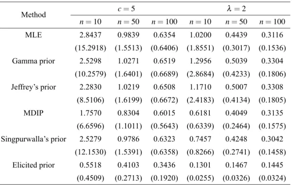
TABLE I

Average bias of the estimates ofcandλand their associated MSEs (in parenthesis) for the different

methods withccc===333andλλλ===000...020202.

Method c=3 λ =0.02

n=10 n=50 n=100 n=10 n=50 n=100

MLE 0.8476 0.3080 0.2077 0.0196 0.0088 0.0060

(1.4217) (0.1556) (0.0685) (0.0009) (0.0001) (6.0e-05)

Gamma prior 0.6607 0.2935 0.1997 0.0363 0.0097 0.0062

(0.6696) (0.1378) (0.0649) (0.0042) (0.0002) (6.9e-05)

Jeffrey’s prior 0.5204 0.2907 0.1978 0.0360 0.0096 0.0061

(0.4204) (0.1341) (0.0613) (0.0037) (0.0001) (6.8e-05)

MDIP 0.5639 0.2749 0.1913 0.0573 0.0114 0.0068

(0.4732) (0.1178) (0.0570) (0.0063) (0.0002) (8.4e-05)

Singpurwalla’s prior 0.4687 0.2898 0.1780 0.0248 0.0091 0.0058

(0.3387) (0.1327) (0.0494) (0.0015) (0.0001) (6.2e-05)

Elicited prior 0.2146 0.1822 0.1528 0.0040 0.0045 0.0040

(0.0680) (0.0538) (0.0367) (2.5e-05) (3.2e-05) (2.5e-05)

for Table II, t25 = 0.1083,t50 = 0.2010,t75 = 0.2992 and t90 = 0.3820 resulting (a1,a2,b1,b2) =

(23.3800,4.2410,23.3795,11.9681) and for Table III witht25 =0.2272,t50 =0.4348,t75 =0.6638 and

t90=0.8618provides(a1,a2,b1,b2) = (38.7505,17.2753,13.2237,13.5219). Frequentist property of

cov-erage probabilities for the parameters c andλ have also been obtained to compare the Bayes estimators with different priors and MLE. Tables IV, V and VI summarize the simulated coverage probabilities of 95% confidence/ credible intervals.

From the simulation results, we reach to the following conclusions:

1. With increase in sample size, biases and MSEs of the estimators decrease for given values ofn,candλ. 2. The performance of the MLEs are quite satisfactory. The Bayes’ estimates using noninformative prior works quite well, and in most of the cases it performs better, in terms of MSE than the MLE when the value ofλ is very small.

3. Bayes estimates based on elicited prior produces much smaller bias and MSE than using the other assumed priors.

4. For the three sample sizes considered here, the elicited prior produces an over-coverage probability for small sample sizes while MLE and independent gamma priors seem to have an under-coverage for some cases. Coverage probabilities are very close to the nominal value when n increases.

AN EXAMPLE WITH LITERATURE DATA

TABLE II

Average bias of the estimates ofcandλ and their associated MSEs (in parenthesis) for the different

methods withccc===555andλλλ===222.

Method c=5 λ =2

n=10 n=50 n=100 n=10 n=50 n=100

MLE 2.8437 0.9839 0.6354 1.0200 0.4439 0.3116

(15.2918) (1.5513) (0.6406) (1.8551) (0.3017) (0.1536)

Gamma prior 2.5298 1.0271 0.6519 1.2956 0.5039 0.3304

(10.2579) (1.6401) (0.6689) (2.8684) (0.4233) (0.1806)

Jeffrey’s prior 2.2830 1.0219 0.6508 1.1710 0.5007 0.3308

(8.5106) (1.6199) (0.6672) (2.4183) (0.4134) (0.1805)

MDIP 1.7570 0.8304 0.6015 0.6181 0.4049 0.3135

(6.6596) (1.1011) (0.5643) (0.6339) (0.2464) (0.1575)

Singpurwalla’s prior 2.5279 0.9786 0.6323 0.7457 0.4248 0.3042

(12.1530) (1.5391) (0.6358) (0.8266) (0.2741) (0.1458)

Elicited prior 0.5518 0.4103 0.3436 0.1301 0.1467 0.1445

(0.4509) (0.2713) (0.1920) (0.0255) (0.0326) (0.0324)

Let us consider the following data set provided in King et al. (1979):

112, 68, 84, 109, 153, 143, 60, 70, 98, 164, 63, 63, 77, 91, 91, 66, 70, 77, 63, 66, 66, 94, 101, 105, 108, 112, 115, 126, 161, 178.

These data represent the numbers of tumor-days of 30 rats fed with unsaturated diet. Chen (1997) and Asgharzadeh and Abdi (2011) used the Gompertz distribution for these data set in order to obtain exact confidence intervals and joint confidence regions for the parameters based on two different statistical anal-ysis. Let us also assume the Gompertz distribution with density (1) fitted to the data and to compare the performance of the methods discussed in this paper.

For a Bayesian analysis, we assume independent Gamma prior distributions for the parameterscandλ, with the hyper parameter valuesa=b=α=β =0.01. The Bayes estimates cannot be obtained in closed

form therefore we use MCMC procedure to compute the Bayes estimates and also to construct credible intervals. Using the software R, we simulated 50,000 MCMC samples (5,000 “burn-in-samples”) for the joint posterior distribution. The convergence of the chains was monitored from trace plots of the simulated samples. The estimates and 95% confidence intervals under classical method and Bayesian estimates with 95% credible intervals for the parameterscandλ of the Gompertz distribution are given in Table VII. The results show that among the Bayes estimators, Bayes estimate based on Singpurwalla’s prior performs the best in terms of credible intervals for both the parameters.

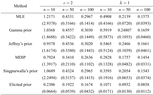
TABLE III

Average bias of the estimates ofcandλand their associated MSEs (in parenthesis) for the different

methods withccc===222andλλλ===111.

Method c=2 λ=1

n=10 n=50 n=100 n=10 n=50 n=100

MLE 1.2171 0.4331 0.2967 0.4908 0.2139 0.1575

(2.9378) (0.3166) (0.1414) (0.4166) (0.0720) (0.0393)

Gamma prior 1.0368 0.4557 0.3030 0.5919 0.24807 0.1659

(1.8688) (0.3422) (0.1449) (0.5873) (0.1055) (0.0460)

Jeffrey’s prior 0.9578 0.4536 0.3020 0.5465 0.2466 0.1661

(1.6174) (0.3380) (0.1443) (0.5124) (0.1039) (0.0461)

MDIP 0.7924 0.3410 0.2636 0.2828 0.1757 0.1454

(1.3917) (0.2110) (0.1102) (0.1328) (0.0482) (0.0331) Singpurwalla’s prior 1.0689 0.4324 0.2965 0.3593 0.2054 0.1543

(2.2494) (0.3157) (0.1415) (0.1916) (0.0653) (0.0374)

Elicited prior 0.2306 0.1922 0.1674 0.1071 0.0932 0.0858

(0.0664) (0.0539) (0.0432) (0.0171) (0.0130) (0.0112)

TABLE IV

Coverage probabilities for the parameterscccandλλλ.

Method c=3 λ =0.02

n=10 n=50 n=100 n=10 n=50 n=100

MLE 0.95 0.95 0.95 0.73 0.87 0.91

Gamma prior 0.91 0.92 0.92 0.91 0.92 0.92

Jeffrey’s prior 0.97 0.96 0.96 0.97 0.96 0.96

MDIP 0.94 0.95 0.96 0.93 0.95 0.96

Singpurwalla’s prior 0.97 0.96 0.98 0.98 0.96 0.98

Elicited prior 1.00 0.98 0.98 1.00 0.99 0.98

CONCLUSIONS

TABLE V

Coverage probabilities for the parameterscccandλλλ.

Method c=5 λ =2

n=10 n=50 n=100 n=10 n=50 n=100

MLE 0.90 0.97 0.96 0.82 0.92 0.95

Gamma prior 0.89 0.96 0.95 0.89 0.96 0.94

Jeffrey’s prior 0.95 0.95 0.95 0.95 0.95 0.95

MDIP 0.97 0.97 0.96 0.98 0.97 0.95

Singpurwalla’s prior 0.94 0.95 0.96 0.92 0.93 0.95

Elicited prior 1.00 0.99 0.99 1.00 1.00 0.99

TABLE VI

Coverage probabilities for the parameterscccandλλλ.

Method c=2 λ =1

n=10 n=50 n=100 n=10 n=50 n=100

MLE 0.92 0.96 0.95 0.84 0.93 0.94

Gamma prior 0.90 0.95 0.94 0.92 0.93 0.94

Jeffrey’s prior 0.96 0.94 0.94 0.95 0.94 0.94

MDIP 0.97 0.96 0.95 0.98 0.96 0.95

Singpurwalla’s prior 0.94 0.94 0.94 0.92 0.94 0.94

Elicited prior 1.00 0.99 0.99 1.00 0.99 0.98

TABLE VII

Estimators and 95% confidence/credible intervals ofcccandλλλof the Gompertz distribution

for different estimation methods.

Method cb 95% CI bλ 95% CI

MLE 0.0241 (0.0160, 0.0322) 0.0016 (0.0002, 0.0031) Gamma Prior 0.0232 (0.0150, 0.0312) 0.0019 (0.0007, 0.0038) Jeffrey’s prior 0.0234 (0.0152, 0.0318) 0.0018 (0.0007, 0.0038) MDIP 0.0226 (0.0147, 0.0304) 0.0020 (0.0008, 0.0045) Singpurwalla’s Prior 0.0242 (0.0165, 0.0317) 0.0016 (0.0006, 0.0033)

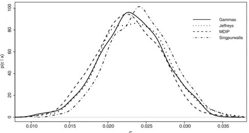
0.010 0.015 0.020 0.025 0.030 0.035

0

20

40

60

80

100

c

p(c | x)

Gammas Jeffreys MDIP Singpurwalla

Figure 2 -The posterior densities for the parametercof the Gompertz distribution fitted by the data.

0.000 0.001 0.002 0.003 0.004 0.005

0

100

200

300

400

500

600

λ

p(

λ

| x)

Gammas Jeffreys MDIP Singpurwalla

Figure 3 -The posterior densities for the parameterλof the Gompertz distribution fitted by the data.

priors and also provides an over-coverage probability than their counterparts. Hence, we can conclude that, in the situation of the absence of information, the MDIP prior is more indicate for a Bayesian estimation of the two-parameter Gompertz distribution. On the other hand, in the situation where we have available expert’s information, the Elicited prior will perform the best estimators.

REFERENCES

ASGHARZADEH A AND ABDI M. 2011. Exact Confidence Intervals and Joint Confidence Regions for the Parameters of the Gompertz Distribution based on Records. Pak J Statist 271: 55-64.

BERNARDO JM. 1979. Reference Posterior Distributions for Bayesian Inference. J R Stat Soc Series B Stat Methodol 41: 113-147. CASELLA G AND BERGER RL. 2001. Statistical Inference. Cengage Learning, 660 p.

CHEN Z. 1997. Parameter estimation of the Gompertz population. Biom J 39: 117-124.

ELANDT-JOHNSON RC AND JOHNSON NL. 1979. Survival Models and Data Analysis. J Wiley & Sons: NY, 457 p. FRANSES PH. 1994. Fitting a Gompertz curve. J Oper Res Soc 45: 109-113.

GOMPERTZ B. 1825. On the nature of the function expressive of the law of human mortality and on a new mode of determining the value of life contingencies. Philos Trans R Soc Lond 115: 513-583.

ISMAIL AA. 2010. Bayes estimation of Gompertz distribution parameters and acceleration factor under partially accelerated life tests with type-I censoring. J Stat Comput Simul 80: 1253-1264.

ISMAIL AA. 2011. Planning step-stress life tests with type-II censored Data. Sci Res Essays 6: 4021-4028.

JAHEEN ZF. 2003a. Prediction of Progressive Censored Data from the Gompertz Model. Commun Stat Simul Comput 32: 663-676. JAHEEN ZF. 2003b. A Bayesian analysis of record statistics from the Gompertz model. Appl Math Comput 145: 307-320. JEFFREYS SIR HAROLD. 1967. Theory of probability. Oxford U Press: London, 470 p.

KIANI K, ARASAN J AND MIDI H. 2012. Interval estimations for parameters of Gompertz model with time-dependent covariate and right censored data. Sains Malays 414: 471-480.

KING M, BAILEY DM, GIBSON DG, PITHA JV AND MCCAY PB. 1979. Incidence and growth of mammary tumors induced by 7, l2-Dimethylbenz antheacene as related to the dietary content of fat and antioxidant. J Natl Cancer Inst 63: 656-664. LAWLESS JF. 2003. Statistical Models and Methods for Lifetime Data. J Wiley & Sons: New Jersey, 664 p.

LENART A. 2014. The moments of the Gompertz distribution and maximum likelihood estimation of its parameters. Scand Actuar J 3: 255-277.

LENART A AND MISSOV TI. 2016. Goodness-of-fit tests for the Gompertz distribution. Commun Stat Theory Methods 45: 2920-2937.

MAKANY RA. 1991. Theoretical basis of Gompertz’s curve. Biom J 33: 121-128.

MEIJER CS. 1936. Über Whittakersche bzw. Besselsche Funktionen und deren Produkte. Nieuw Archief voor Wiskunde 18: 10-39. MILGRAM M. 1985. The generalized integro-exponential function. Math Comp 44: 443-458.

RAO BR AND DAMARAJU CV. 1992. New better than used and other concepts for a class of life distribution. Biom J 34: 919-935. READ CB. 1983. Gompertz Distribution. Encyclopedia of Statistical Sciences. J Wiley & Sons, NY.

SHANUBHOGUE A AND JAIN NR. 2013. Minimum Variance Unbiased Estimation in the Gompertz Distribution under Progressive Type II Censored Data with Binomial Removals. Int Sch Res Notices 2013: 1-7.

SINGH N, YADAV KK AND RAJASEKHARAN R. 2016. ZAP1-mediated modulation of triacylglycerol levels in yeast by transcriptional control of mitochondrial fatty acid biosynthesis. Mol Microbiol 1001: 55-75.

SINGPURWALLA ND. 1988. An interactive PC-based procedure for reliability assessment incorporating expert opinion and survival data. J Am Stat Assoc 83: 43-51.

TIBSHIRANI R. 1989. Noninformative Priors for One Parameters of Many. Biometrika 76: 604-608.

WILLEKENS F. 2002. Gompertz in context: the Gompertz and related distributions. In: Tabeau E, Van den Berg JA and Heathcote C (Eds), Forecasting mortality in developed countries - insights from a statistical demographic and epidemiological perspective European studies of population. Dordrecht: Kluwer Academic Publishers 9: 105-126.

WU JW, HUNG WL AND TSAI CH. 2004. Estimation of parameters of the Gompertz distribution using the least squares method. Appl Math Comput 158: 133-147.

WU JW AND LEE WC. 1999. Characterization of the mixtures of Gompertz distributions by conditional expectation of order statistics. Biom J 41: 371-381.

WU JW AND TSENG HC. 2006. Statistical inference about the shape parameter of the Weibull distribution by upper record values. Stat Pap 48: 95-129.

WU SJ, CHANG CT AND TSAI TR. 2003. Point and interval estimations for the Gompertz distribution under progressive type-II censoring. Metron LXI: 403-418.

ZELLNER A. 1977. Maximal Data Information Prior Distributions. In: Aykac A and Brumat C (Eds), New Methods in the applications of Bayesian Methods. North-Holland Amsterdam, p. 211-232.

ZELLNER A. 1984. Maximal Data Information Prior Distributions. Basic Issues in Econometrics, U. of Chicago Press.

ZELLNER A. 1990. Bayesian Methods and Entropy in Economics and Econometrics. In: Grandy Junior WT and Schick LH (Eds), Maximum Entropy and Bayesian Methods Dordrecht Netherlands: Kluwer Academic Publishers, p. 17-31.