Braz. J. Chem. Eng. vol.31 número3

ISSN 0104-6632 Printed in Brazil

www.abeq.org.br/bjche

Vol. 31, No. 03, pp. 771 - 785, July - September, 2014 dx.doi.org/10.1590/0104-6632.20140313s00002625

Brazilian Journal

of Chemical

Engineering

STATE ESTIMATION OF CHEMICAL

ENGINEERING SYSTEMS TENDING TO

MULTIPLE SOLUTIONS

N. P. G. Salau

1*

, J. O. Trierweiler

2

and A. R. Secchi

3 1

Chemical Engineering Department, Universidade Federal de Santa Maria, UFSM, Av. Roraima 1000, Cidade Universitária, Bairro Camobi, CEP: 97105-900 Santa Maria, RS - Brazil.

Phone: + (55) (55) 3220-8448, Fax: + (55) (55) 3220-8030 E-mail: ninasalau@ufsm.br

2_{Chemical Engineering Department, Universidade Federal do Rio Grande do Sul, Porto Alegre - RS, Brasil} 3

Chemical Engineering Program, COPPE, Universidade Federal do Rio de Janeiro, Rio de Janeiro - RJ, Brasil.

(Submitted: March 26, 2013 ; Revised: September 5, 2013 ; Accepted: September 27, 2013)

Abstract - A well-evaluated state covariance matrix avoids error propagation due to divergence issues and, thereby, it is crucial for a successful state estimator design. In this paper we investigate the performance of the state covariance matrices used in three unconstrained Extended Kalman Filter (EKF) formulations and one constrained EKF formulation (CEKF). As benchmark case studies we have chosen: a) a batch chemical reactor with reversible reactions whose system model and measurement are such that multiple states satisfy the equilibrium condition and b) a CSTR with exothermic irreversible reactions and cooling jacket energy balance whose nonlinear behavior includes multiple steady-states and limit cycles. The results have shown that CEKF is in general the best choice of EKF formulations (even if they are constrained with an ad hoc clipping strategy which avoids undesired states) for such case studies. Contrary to a clipped EKF formulation, CEKF incorporates constraints into an optimization problem, which minimizes the noise in a least square sense preventing a bad noise distribution. It is also shown that, although the Moving Horizon Estimation (MHE) provides greater robustness to a poor guess of the initial state, converging in less steps to the actual states, it is not justified for our examples due to the high additional computational effort.

Keywords: Nonlinear state estimation; State covariance matrix; Noise distribution; Multiple solutions.

INTRODUCTION

It is well known that a suitable design of state es-timators requires a representative model for captur-ing the plant behavior and knowledge about the noise statistics, which are generally not known in practical applications (Valappil and Georgakis, 2000). How-ever, some divergence issues such as numerical round-off, plant-model mismatch, and state unob-servability also deserve special attention because they can lead to convergence failures (Brown and Hwang, 2012; Grewal and Andrews, 2008; Simon,

2006). Any state covariance matrix equation is com-posed of states, measurements, linear models and noise covariance statistics and, hence, all the men-tioned divergence issues may increase the error propagation conveyed by this matrix.

is much less straightforward. The model accuracy is specified by tuning the Kalman filter that involves the selection of the process-noise covariance matrix. If this matrix is guessed low, the filter will believe the model excessively and will not use the on-line measurements properly to correct the states. This can lead to poor performance or even filter divergence. On the other hand, if the process-noise covariance matrix is guessed higher than the actual value, the state estimates will be noisy and uncertain, as this would lead to increased values of the state covari-ance matrix (Valappil and Georgakis, 2000; Salau et al., 2013). In a few words, choosing the right value of the tuning parameters is very important for suc-cessful application of EKF (Kalman, 1962).

In contrast to the measurement noise covariance, information about the uncertainty of the initial state guess cannot be measured experimentally. In gen-eral, the filter will not be fatally affected if the initial state guess is not close to the actual initial state, but convergence to the correct estimate may be slow. However, if the initial state estimate covariance ma-trix is chosen too small or optimistic while initial state guess and actual initial state differ considerably, the Kalman filter gain becomes small and the esti-mator relies on the model predictions more than it should.

Thus, subsequent measurements do not have the impact on the estimator that they need to have. The filter might then learn the wrong state too well and diverge (Jazwinski, 1970). The importance of choos-ing a consistent pair of an initial state estimate guess and initial state estimate covariance matrix is also em-phasized by other authors (Valappil and Georgakis, 2000). For instance, Vachhani et al. (2004) empha-sized the role of a consistent choice of initial state estimate covariance matrix and consequently the use of alternate initial state information for their simula-tions. Similarly, Prakash et al. (2010) silently adapt their initial state estimate to be more consistent with the original initial state estimate covariance matrix.

In this work, however, we will show that some EKF formulations can indeed converge, even in the presence of poor initial guesses, as well as a poor initial state estimate covariance matrix.

In the literature, several modified implementa-tions of the EKF are presented in an effort to avoid the filter failure (Grewal and Andrews, 2008). The basic difference between these formulations is con-cerned with the state covariance matrix computation. We can also find in the literature some contributions which show examples and outline conditions where other methods perform better than the standard EKF, MHE for instance (Rao and Rawlings, 2002;

Haseltine and Rawlings, 2005). Otherwise, these works address comparison issues such as accuracy and computational expense and no efforts are made to avoid divergence or even instability by EKF state covariance matrix computation and thereby improve the filter performance.

Due to the lack of literature concerning this problem, we investigate in this paper the perform-ance of four EKF formulations, being three uncon-strained: (i) the classical EKF formulation, called here discrete EKF (DEKF), (ii) EKF with the con-tinuous Riccati equation (EKF-CRE) and (iii) re-duced-rank extended Kalman filter (RREKF); and a constrained EKF (CEKF) formulation (Gesthuisen et al., 2001) to derive some results with two systems tending to multiple solutions giving insights into their numerical performance: a) a batch chemical reactor with reversible reactions whose system model and measurement are such that multiple states satisfy the equilibrium condition and b) a CSTR with exothermic irreversible reactions and cooling jacket energy balance whose nonlinear behavior includes multiple steady-states and limit cycles.

In the next section we briefly review the state es-timation formulations of interest. Then, we present two systems tending to multiple solutions and outline conditions that lead a classical EKF formulation to converge to physically unrealizable equilibrium points and to an undesired steady-state. Then, we demonstrate the potentiality of EKF-CRE and RREKF to handle the divergence issues by state covariance matrix computation. Otherwise, both for-mulations may not prevent undesired states before eventually converging to the actual states. Although an ad hoc clipping strategy seems to be a reasonable solution to constrain the states, it disregards the as-sumption that the measurement noise is a Gaussian random noise.

Finally, we have shown that CEKF is in general the best alternative to EKF formulations due to the possibility of incorporating constraints into an opti-mization problem, hence preventing the estimator from converging to undesired states and from bad noise distribution. Furthermore, this technique de-mands a small computational effort and a perform-ance comparable to the MHE.

FORMULATION AND SOLUTION OF THE ESTIMATION PROBLEM

State Estimation of Chemical Engineering Systems Tending to Multiple Solutions 773

(

, ,

)

( )

x= f x u t +ω t (1)

(

,

)

k k k k k

y =h x t +ν (2)

( )

t ≈N

(

0,Q

)

ω (3)

(

0,

)

k ≈N Rk

ν (4)

where u denotes the deterministic inputs, x denotes the states, and y denotes the measurements. The process-noise vector, ω

( )

t , and the measurement-noise vector,

k

ν

, are assumed to be white Gaussian random proc-esses with zero mean and covariance Q and Rk,

re-spectively.

The system is linearized at each time step to ob-tain the local state-space matrices as below:

1 ˆ k k

k k

f F

x x ₋

∂ ⎛ ⎞

= ⎜_{⎝ ∂} ⎟_⎠ (5)

1 ˆ k k

k k

h H

x x ₋

∂ ⎛ ⎞

= ⎜_{⎝ ∂} ⎟_⎠ (6)

The filter algorithm is initialized by the initially expected state and state covariance:

( )

0 |0

ˆ 0

x = ⎡E x_⎣ ⎤_⎦ (7)

( )

(

)

(

( )

)

0 |0 0 ˆ0 |0 0 ˆ0 |0

T

P =E⎡_⎢ x −x x −x ⎤_⎥

⎣ ⎦ (8)

Unconstrained EKF Formulations

The equations that compose the different steps in the considered unconstrained EKF formulations are given below.

State transition equation:

(

)

1 1 1 ₁

ˆ_{k k} ˆ_{k k} k ˆ, ,

k

x ₋ x _{− −} f x u d

−

= +

_∫

τ τ (9)

Kalman gain equation:

1

1 1

T T

k k k k k k k k k

K =P ₋H _⎣⎡H P ₋H +R ⎤_⎦− (10)

State update equation:

(

)

1 1

ˆ_{k k} ˆ_{k k k k} ˆ_{k k} , _k

x =x ₋ +K _⎣⎡y −h x ₋ t ⎤_⎦ (11)

The basic difference of these formulations is con-cerned with the state covariance matrix computation, as described below.

Discrete Extended Kalman Filter

DEKF considers discrete-time dynamics and dis-crete-time measurements. This situation is often encountered in practice. Even if the underlying sys-tem dynamics are continuous-time, the state estima-tor usually needs to be implemented in a digital computer (Simon, 2006).

The nonlinear dynamic system in continuous time (cf. Eq. (1)) can be approximated by a linear dy-namic system in continuous time expressed in a gen-eral form as a first-order vector of difference equa-tion (Brown and Hwang, 2012; Grewal and Andrews, 2008; Simon, 2006).

1 1 1

k k k k

x =

ϕ

₋x ₋ +

ω

₋ (12)

where

ϕ

_k−1 is the state transition matrix for the state at time tk given as

(

1

)

1 k k

k

F t t e − −

− =

ϕ (13)

The state covariance matrix transition equation of the DEKF is given by

1 1 1

1 1 1

T

k k k

k k k k

P ₋ =ϕ ₋P_{− −}ϕ ₋ +Q ₋ (14)

and the state covariance matrix update equation can be represented by one of the following equations:

[

]

1

[

]

T

n k k n k k

k k k k

T k k k

P I K H P I K H

K R K

−

= − −

+

(15)

1

1 1 1

1

−

− − −

−

⎡ ⎤

= − T_⎣ T+ _⎦

k k k k

k k k k k k k k

k k k

P P P H H P H R

H P (16)

[

n k k

]

1

k k k k

The first equation (Eq. (15)), called the Joseph form (Brown and Hwang, 2012; Grewal and Andrews, 2008; Simon, 2006), has somewhat better numerical behavior than the other forms in unusual numerical situations (Brown and Hwang, 2012) since it guar-antees that P_{k k}will always be symmetric positive definite, as long as P_{k k−1} is symmetric positive defi-nite, and Kk does not need to be optimal. The third

equation for P_{k k}(Eq. (17)) is computationally simpler than the first equation, but its form does not guarantee symmetry or positive definiteness for P_{k k}

(Simon, 2006). However, we have formulated the DEKF using the Eq. (17) for comparison with the reference of our first case study (Haseltine and Rawlings, 2005). Equation 16 is just the substitution of Eq. (10) into Eq. (17) and is rarely implemented as written above (Simon, 2006), but will be useful in our derivation of the information filter in the next sections.

Reduced Rank Extended Kalman Filter

The reduced rank extended Kalman filter (RREKF) expresses the transition state covariance matrix in terms of its dominant eigenvectors. Ne-glecting non-dominant eigenvectors of the covari-ance matrix implies that the dimensionality of the confidence region is reduced. Measurement updates therefore have no effect on the directions of non-dominant eigenvectors. If the actual state does not leave the attractor, the RREKF is advantageous since measurement updates are omitted in those directions of strongest attraction. Furthermore, this EKF modi-fication is more robust against improper initializa-tion, as claimed by Pham et al (1998).

Although the RREKF is not applied or at least barely applied to chemical processes, we have se-lected this formulation to show the benefits of a lower rank covariance approximation of the transi-tion state covariance matrix (Eq. (14)) in the exam-ples we are interested in. Except for this modifica-tion, RREKF presents the same formulation as for DEKF.

We briefly outline the implementation and impli-cations of the low-rank covariance approximation. Let

V

_{P k,} comprise the eigenvectors

υ

_{P i,} of P_{k k−1}

as columns and

Λ

_{P k,} the corresponding eigenvalues

, P i

λ

on the diagonal. As the transition state covari-ance matrix (Eq. (14)) is symmetric, it can be de-composed as

, , , , , ,

1

1 n

T T

P k P k P i P i P i P i k k

i

P ₋ V V

=

= Λ =

∑

λ υ υ (18)

For λ_P,1 < λ_P,2 <"< λ_{P n,} , the rank q < n

approximation of the covariance matrix is given by

, , ,

, 1

1 q

T P i P i P i q k k

i

P ₋

=

=

∑

λ υ υ (19)

Geometrically, the lower-rank approximation is the orthogonal projection of the covariance ellipse or (hyper-)ellipsoid onto its q most dominant axes.

Extended Kalman Filter with the Continuous-Time Riccati Equation

In this section we introduce an EKF formulation referred to as EKF with the continuous-time Riccati equation (EKF-CRE).

Before we define the EKF-CRE, a brief review about an alternate form for the EKF which applies the discrete-time Riccati equation (DRE) is neces-sary (Simon, 2006). This approximation referred to here as EKF-DRE is computationally attractive be-cause the state covariance matrix, P, is evaluated just once at each time step, i. e. the state covariance ma-trix transition and update steps are carried out si-multaneously.

Considering Eq. (16) for the state covariance ma-trix update, rewritten here for convenience:

1

1 1 1

1

−

− − −

−

⎡ ⎤

= − T_⎣ T+ _⎦

k k k k

k k k k k k k k

k k k

P P P H H P H R

H P (20)

Applying Eq. (14) considering the next time steps, we can write the state covariance matrix tran-sition as follows:

1

T

k k k

k k k k

P₊ =ϕ P ϕ +Q (21)

Substituting Eq. (20) into Eq. (21) gives

1 1

1 1

1 1

− −

− +

− −

⎛ − ⎞

⎜ ⎟

=

⎜⎡ ₊ ⎤ ⎟

⎣ ⎦

⎝ ⎠

+

T k

k k k k

k

k k T

k k k k k k k k

T

k k

P P H

P

H P H R H P

Q

ϕ

ϕ (22)

State Estimation of Chemical Engineering Systems Tending to Multiple Solutions 775

1 + k k

P , because the state covariance matrix transition

1

(P_{k+ k}) and update (P_k+1k+1) steps are carried out simultaneously, we obtain the equation for the one-step state covariance matrix equation

1 1 1 + + − = ⎡ ⎤ − _⎣ + _⎦ + T k k

k k k k

T T

k k k k k k k k k

T

k k k k k

P P

P H H P H R

H P Q

ϕ ϕ

ϕ

ϕ

(23)

Now, rewriting Eq. (23), considering one time step before, we arrive to the formulation called DRE

1 1 1 1

1

1 1 1 1 1

1 1 1 1 − − − − − − − − − − − − − − = ⎡ ⎤ − _⎣ + _⎦ + T k k

k k k k

T T

k k k k k k k k k T

k k k k k

P P

P H H P H R

H P Q

ϕ

ϕ

ϕ

ϕ

(24)

Note that the Kalman gain (Eq. (10)) requires

1 k k

P ₋ and this term is not computed in this alternate EKF formulation. Thus, Eq. (10) can be modified by assuming that P_{k k−1}=P_{k−1 k−1}, resulting in

1

1 1 1 1

T T

k k k k k k k k k

K P H H P H R

−

− − ⎡ − − ⎤

= _⎣ + _⎦ (25)

In spite of applying the one-step state covariance matrix equation and using a different equation for the Kalman gain, the EKF-DRE and the DEKF result in identical results and estimation-error covariances (Simon, 2006). To avoid a redundancy, the EKF-DRE will be not compared in our examples.

Alternatively, following the same steps, we can write a similar expression for the continuous case, which can be written as follows:

( ) ( )

( ) ( )

( )

( ) ( ) ( )

( ) ( )

1 1 1 1 − − − − = ⎡ _{+ +} ⎤ + ⎢ ⎥ − ⎢ ⎥ ⎣ ⎦

∫

k k k k

T k

T k

P P

F P P F Q

d

P H R H P

τ τ τ τ τ _τ τ τ τ τ τ

(26)

The equation above is known as the continuous-time Ricatti equation (CRE). It is equivalent to the state covariance matrix transition equation of the continuous-time EKF found in the literature (Brown and Hwang, 2012; Grewal and Andrews, 2008; Simon, 2006). The basic difference between both formulations is concerned with the Kalman gain equation. For the continuous-time EKF, the Kalman gain equation considers that the measurement values remain constant during the entire time interval, which is suitable just for small sampling times. Fur-thermore, the EKF-CRE considers continuous-time dynamics and discrete observation for update, i. e. discrete-time measurements.

Moving Horizon Estimator (MHE)

Before explaining the CEKF formulation, the ba-sic aspects of the MHE (Muske and Rawlings, 1994; Robertson et al., 1996; Rao et al., 2003) are pre-sented. As paper of Haseltine and Rawlings (2005), we examine the performance of MHE with local optimization and an arrival cost approximated with a smoothing update (Tenny and Rawlings, 2002). According to Tenny and Rawlings (2002) the smoothing scheme is superior to the filtering scheme because the filtering scheme induces oscillations in the state estimates through the unnecessary propaga-tion of initial error. Further details regarding this MHE scheme can be found in the mentioned manuscript.

The basic idea of MHE is to proceed with state estimation by using only the most recent N+1 measurements, where N is the time horizon size.

The moving horizon approximation of the objec-tive function is given by

(

)

(

)

( )

k N 1 k k 1 k k N k k k

1

1 _{1 1}

1

1 1 1 1

ˆ ˆ ˆ ˆ ˆ ˆ

ω , ,ω

ν , ,ν

min

− − − − − − _{− −} − − − − − − − − = − = − ⎡ ⎤ =⎢ + + ⎥ ⎢ ⎥ ⎣ ⎦

Ψ

_∑

_∑

" "

k k

T T T

k k

k N k k N k k N k j k j k j k j k

j k N j k N

N

P Q R

subject to the equality constraints

(

)

( )

1 1 1 1 ˆ ˆ ˆ ˆ

ˆ ˆ, , , , , 1

ˆ

ˆ , , ,

− − − − − + + = + = + = − − = + = −

∫

" "

k N k k N k k N k

j

j k _j j k

j j k j k

x x

x f x u d j k N k

y h x j k N k

ω

τ τ ω

ν

(28)

and the inequality constraints

min max

min 1 max

min max

ˆ

ˆ ˆ ˆ , , ,

ˆ ˆ ˆ , , ,

j k

j k

j k

x x x

j k N k

j k N k

− ≤ ≤ ≤ ≤ = − ≤ ≤ = − " "

ω ω ω

ν ν ν

(29)

From optimization, measurements and states are updated as follows

(

)

( )

* 1 1 1 _* 1 * ˆ ˆ ˆ ˆ

ˆ ˆ, , , , , 1

ˆ

ˆ , , ,

− − − − − + + = + = + = − − = + = −

∫

" "

k N k k N k k N k

j

j k _j j k

j j k j k

x x

x f x u d j k N k

y h x j k N k

ω

τ τ ω

ν

(30)

Rao et al. (2003) suggested computing the state covariance matrix equation P_{k k}N (Eq. (31)) recursively using the discrete Riccati equation. One obtains this result by deriving the deterministic Kalman filter using forward dynamic programming (Cox, 1964).

1 1

1

1 1 1 1

1 1 − − − − − − − − − = ⎡ ⎤ − _⎣ + _⎦ +

N N T

k k

k k k k

N T N T

k k k k k k k k k

N T

k k k k k

P P

P H H P H R

H P Q

ϕ ϕ

ϕ

ϕ

(31)

Note that the equation above is the same as for Eq. (24) applied to each horizon step.

We solve Eq. (27) using sequential quadratic pro-gramming (SQP) as implemented in the medium-scale algorithm of the fmincon function in MatLab. For the successive integration of Eq. (30) we use DASSLC (Differential-Algebraic System Solver in C) which does the multirate integration of systems of differential-algebraic equations (DAEs). The inte-gration algorithm used in DASSLC is an extension

of the DASSL code of Petzold (1983) to address high-index and large-scale problems, and the setup algorithm used in DASSLC is based on the DAWRS code (Secchi et al., 1991), a package to solve DAEs on parallel machines.

Constrained EKF

CEKF follows from the MHE when the horizon length is set to zero (Gesthuisen et al., 2001). Zero length implies that ODEs are not considered in the optimization problem, which simplifies the com-plexity of solving a nonlinear dynamic optimization problem.

Setting (N=0) in the MHE optimization problem (Eq. (27)), the resulting formulation is exactly the CEKF formulation problem:

(

)

( )

k 1 k k k

1

1 1 1

1 1

ˆ min

ω ,ν

ˆ ˆ ˆ

− − − − − − − ⎡ ⎤ ⎢ ⎥ = ⎢ ⎥ + ⎢ ⎥ ⎣ ⎦

Ψ

kT k k k

T k

k k k k k k

P k

R

ω

ω ν ν (32)

subject to the equality constraints:

( )

1 ˆ 1

ˆ ˆ

ˆ ˆ

k k k k k k

k k k k k

x x

y h x

− − = + = + ω ν (33)

and inequality constraints:

min max

min 1 max

min max

ˆ

ˆ ˆ ˆ

ˆ ˆ ˆ

k k

k k

k k

x x x

−

≤ ≤ ≤ ≤ ≤ ≤

ω ω ω

ν ν ν

(34)

From optimization, measurements and states are updated as follows:

( )

* 1 1 * ˆ ˆ ˆ ˆ ˆ

k k k k k k

k k k k k

x x

y h x

− − = + = + ω ν (35)

If the measurement equation is linear, the result-ing problem is a quadratic program (QP), which can be solved with small computational effort (Gesthuisen

State Estimation of Chemical Engineering Systems Tending to Multiple Solutions 777 1

ˆ ˆ ˆ

min

k k

T T

k k k kS k k d k k

k

−

Θ

Ψ

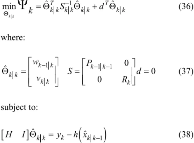
= Θ Θ + Θ (36)

where:

1 1 1 0

ˆ ₀

0

k k k k

k k

k k k

w P

S d

v _R

− _{− −}

⎡ ⎤ ⎡ ⎤ Θ =⎢ ⎥ =⎢ ⎥ =

⎢ ⎥ ⎢_⎣ ⎥_⎦ ⎣ ⎦

(37)

subject to:

[

H I

]

Θˆk k =yk−h x

( )

ˆk k−1 (38)

In contrast to the unconstrained EKF formula-tions, state estimation with CEKF is formulated as an optimization problem, so that constraints on state variables can be incorporated in this problem. Fur-thermore, it is not necessary to compute the Kalman gain (Eq. (10)) and therefore the state covariance matrix P is computed using the discrete Riccati equation as in Eq. (24).

Although the CEKF belongs to a family of MHE estimators, we choose to call this formulation here CEKF, as introduced by Gesthuisen et al. (2001). Note that CEKF is similar to EKF because the latter also takes into account a zero-length horizon in the updating stage, i. e. the current state is estimated only using the current measurement on the horizon and it is equivalent to zero horizon length (N=0). In the absence of any constraints and for low process-noise uncertainties, these formulations are similar.

Afterwards, Vachhani et al. (2005) have proposed essentially the same formulation as for CEKF with a different name: Recursive Nonlinear Dynamic Data Reconciliation (RNDDR). However, we have de-cided to adopt the earlier nomenclature.

EXAMPLES OF DIVERGENCE ISSUES BY STATE COVARIANCE MATRIX

COMPUTATION

In this section, we outline the conditions that gen-erate divergence issues by state covariance matrix computation in two chemical engineering systems. The first one is a batch reactor with reversible reac-tions whose system model and measurement are such that multiple states satisfy the equilibrium condition. The results obtained with this system (Figures 1 to 6) have been published in our previous work (Salau et al., 2009).

The second one is a CSTR with exothermic irre-versible reactions and cooling jacket energy balance whose nonlinear behavior includes multiple steady-states and limit cycles.

System Tending to Multiple Equilibrium Points

The first example was introduced by Haseltine and Rawlings (2005) and consists of a gas-phase batch reactor with multiple equilibrium points con-sidering the following reversible reactions:

1 2 3 4

2

k k k k

A B C

B C

⎯⎯→ ←⎯⎯ ⎯⎯→ ←⎯⎯

+

(39)

The model equations and the model parameters are given below.

1 2

A

A B C

dc

k c k c c

dt = − + (40)

(

2

)

1 2 2 3 4

B

A B C B C

dc

k c k c c k c k c

dt = − − − (41)

2

1 2 3 4

C

A B C B C

dc

k c k c c k c k c

dt = − + − (42)

with

[

k1 k2 k3 k4

]

=

[

0.5 0.05 0.2 0.01

]

(43)

Multiple states satisfy the equilibrium condition for a given measurement, which in this case is the system pressure at the equilibrium, evaluated by the following equation:

(

A B C

)

y= =p c +c +c RT (44)

Table 1 shows the possible theoretical solutions, without measurement or state noise, at the equilib-rium pressure given by the initial state:

[

]

0 0.5 0.05 0

T

x = (45)

Table 1: Batch Reactor Equilibrium Points, No Measurement or Process Noise.

Component EQ1 EQ2 EQ3

cA 0.0122 -0.0267 -1967.4

cB 0.1826 -0.2372 -9.9454

cC 0.6669 1.1257 1978.2

The state estimator parameters and the poor initial guess x₀ used for this example were obtained from Haseltine and Rawlings (2005):

1 0.25

k k

t t t ₋ min

Δ = − = (46)

2 0 0.5 3x3

P = I (47)

2 3x3

0.001

Q= I (48)

2 0.25

R= (49)

[

]

0 0 0 4

T

x = (50)

According to the authors, EKF fails in this exam-ple because the system model and measurement are such that multiple states satisfy the equilibrium con-dition and is given a poor initial guess of the initial state for the estimator. Nonetheless, we cannot assert that EKF fails because two equilibrium points (EQ1 and EQ2 in Table 1) are possible due to the poor and incoherent guesses of the initial state and its covari-ance matrix used in this example, as discussed in the next section.

RESULTS AND ANALYSES Measurement Noise Perturbation

First, uniform and normally distributed random measurement noises were simulated. Either solution

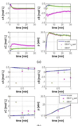
EQ1 or solution EQ2 (i. e. the inconsistent solution) is obtained in accordance with the set of random measurement noise employed in DEKF. Thus, we have chosen a set of random measurement noise which leads DEKF to converge to the solution EQ1 and added a noise measurement perturbation in order to lead it to converge to solution EQ2. As can be seen in Figure 1, a noise measurement perturbation of 0.754 atm at t=0.5 min changes the estimated states trajectory from solution EQ1 to solution EQ2.

We have also found that other divergence issues can lead DEKF to converge to solution EQ2, such as low-precision arithmetic, numeric system lineariza-tion by finite differences, a poor guess of P0 and

incorrect values of the tuning parameters: Q and R.

Comparison Between Unconstrained EKF For-mulations

RREKF and EKF-CRE were applied to the batch reactor in order to prevent the state estimator from converging to EQ2. In spite of a measurement noise

perturbation, both unconstrained EKF formulations converged to solution EQ1, as shown in Figure 2.

(a)

(b)

Figure 1: Comparison between the performances of DEKF with and without a noise measurement per-turbation of 0.754 atm at t=0.5 min: (a) until final batch time and (b) until t=1 min.

State Estimation of Chemical Engineering Systems Tending to Multiple Solutions 779 RREKF disregards non-dominant eigenvectors,

which implies zero variance in the respective direc-tions, and no effect of measurement updates. For this example, we use a rank-two approximation, so the confidence region is an ellipse instead of a (hyper-) ellipsoid, reducing the dimensionality of the confi-dence region. After initial oscillations, the estimated states converge to the actual states. At the equilib-rium point x_eq=

[

0.0124 0.1859 0.6634

]

T, we ob-serve that the eigenvector corresponding to the smallest eigenvalue or the non-dominant eigenvector

[

]

2, -0.9827 0.1677 0.0793 T eq=

υ is orthogonal to the

tangent of the equilibrium curve (the scalar product approaches zero). This eigenvector is not considered in the rank-two covariance approximation and thus the filter applies no correction in this direction or-thogonal to the attractor.

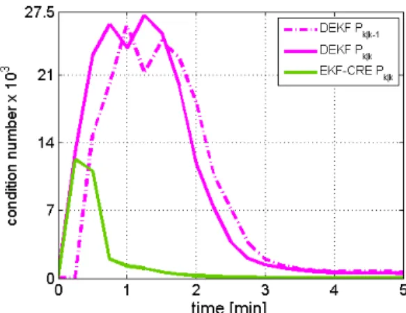
EKF-CRE is not subject to errors due to model discretization. The state covariance matrix computed by EKF-CRE in a single stage (Eq. (26)) guarantees that it will always be symmetric positive definite, since it is derived from the called Joseph form (Brown and Hwang, 2012; Grewal and Andrews, 2008; Simon, 2006), as discussed previously in the present article. Besides, the state covariance matrix of EKF-CRE presents a smaller condition number, i. e. it is less sensitive to perturbations than the states covariance matrices computed by DEKF (eqs 14 and 17), as shown in Figure 3. The mentioned advantages of EKF-CRE over DEKF justify the convergence of this formulation to EQ1, even with a measurement noise perturbation.

Figure 3: Comparison between the condition num-ber of DEKF and EKF-CRE state covariance matri-ces for a system tending to multiple equilibrium points.

Although EKF-CRE and RREKF prevented physically unrealizable states at the final batch time, physically unrealizable states (negative

concentra-tions) were unavoidable during the batch. This fact is justified by the poor guesses of the initial state and its state covariance matrix.

We also considered that the unconstrained for-mulations fail when they converge to negative con-centrations (EQ2) because they do not converge to the given plant measurements (that are consistent with positive concentrations - EQ1), but instead, converge to physically unrealizable states, a fact that could not be considered as a success from the chemi-cal engineering point of view. In the next section it will be shown that constrained formulations can avoid such problems.

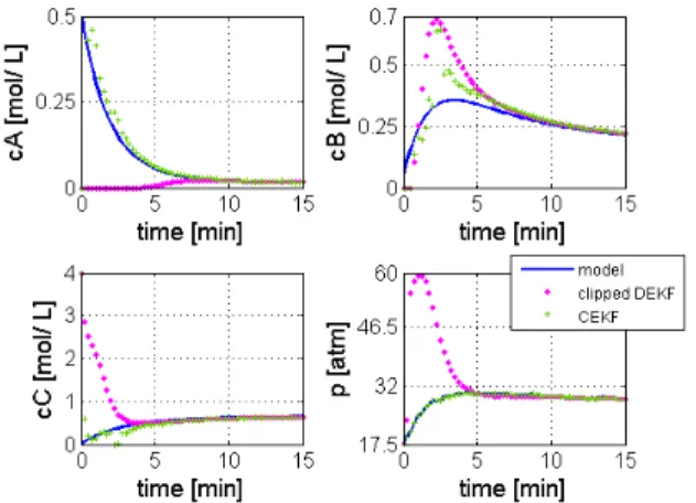
Comparison Between Clipped DEKF and CEKF

To prevent physically unrealizable states, we have constrained DEKF with an ad hoc clipping strategy (Haseltine and Rawlings, 2005) in which negative update values of the state are set to zero (i. e. if xˆ_{k k}< 0, set xˆ_{k k}= 0 ).

The comparison between clipped DEKF and CEKF performances is shown in Figure 4. Note that before eventually converging to the actual states, the pressure filtered by the clipped DEKF is quite larger than the measured one. However, the clipped DEKF in our work presented a better performance when compared with the one presented by Haseltine and Rawlings (2005). In their paper, the clipped DEKF drives the predicted pressure 3 orders of magnitude larger than the measured pressure before eventually converging to the actual states on a longer time scale (1 order larger than the convergence time obtained in our work). This occurred because the authors over-estimated P0 (cf. Eq. (47)). While the initial guess for

the concentration of specie C is too far from its ac-tual value, the same is not valid for the concentration of specie B. Since the authors have chosen a P0 with

the same weight for all initial guesses (diagonal ele-ments of P0), this weight should be balanced

be-tween the initial guesses. We have selected, hence, a lower initial guess of the state covariance matrix:

2 0 0.022 3x3

P = I (51)

Thus, due to a lower initial guess of the state co-variance matrix, the clipped DEKF is shown as a reasonable alternative to prevent physically unrealiz-able states.

state and, thereby, corrects them. Another disadvan-tage of such an approach is that clipped state esti-mates violate the process model, as the negative state estimates were obtained from the model solution.

Figure 4: Comparison between clipped DEKF and CEKF performances for a system tending to multiple equilibrium points until t=30 min.

On the other side, CEKF swiftly converges to the actual states and minimizes

ω

_k and

ν

_k in a least square sense, incorporating constraints into an opti-mization problem, which prevents bad noise distri-bution. Figure 5 illustrates the distribution of

ν

_k for the clipped DEKF and the CEKF. It means that the main difference between the clipped DEKF and CEKF is that the CEKF preserves the gaussianity, which is one of the main assumptions of the Kalman Filter Approach.

Figure 5: Comparison between the distribution of

ν

_k for (a) clipped DEKF (non-Gaussian) and (b) CEKF (Gaussian).

It is well known that the quality of the MHE esti-mates is a function of the estimation horizon (Haseltine and Rawlings, 1970). Thus, we have enlarged the

MHE estimation window to N=2 and compared its performance with the CEKF, as can be seen in Figure 6. In this comparison, CEKF and MHE are computed recursively using the discrete Riccati equation (DRE) (Eq. (31)).

Figure 6: Comparison between CEKF and MHE (N=2) performances for a system tending to multiple equilibrium points until t=15 min.

The Integral Time Absolute Error (ITAE) has been chosen as the performance criterion to compare CEKF and MHE. The results obtained with ITAE, as well as the computational expenses of both filters, are shown in Table 2.

Table 2: Comparison between CEKF and MHE: ITAE and Computational Expenses.

ITAE cA cB cC

average CPU time per time step (s)

CEKF 0.81 4.03 4.74 0.06 MHE (N=2) 0.71 3.24 3.77 2.61 MHE (N=4) 0.69 3.24 3.74 9.42

Even with the MHE considering a size horizon of 4, the average CPU time per time step is smaller than the sampling period (0.25 min). Thus, both CEKF and MHE are suited for this case study.

State Estimation of Chemical Engineering Systems Tending to Multiple Solutions 781

System Tending to Multiple Steady-States and Limit Cycles

As a benchmark example, we have chosen a CSTR, as introduced by Torres and Tlacuahuac (2000). The following two exothermic irreversible first-order reactions in series take place in the reactor:

1 2

k k

A⎯⎯→ ⎯⎯→B C (52)

The reactor volume and physical parameters are assumed to remain constant; perfect mixing is also assumed. In addition the dynamics of the cooling jacket are taken into account.

The dimensionless model equations are given below and the dimensionless parameters are defined in Table 3. More details on the model can be found in Torres and Tlacuahuac (2000).

(

)

( )

1

1f 1 1 3

dx

q x x x x

dτ = − − η φ (53)

(

)

( )

( )

2

2 2 2 2 3 1 3

= _f − − +

dx

q x x x S x x S x

dτ φ η φ η (54)

(

)

(

)

( )

( )

3

3 3 4 3

1 3 2 2 3

= − − −

+ ⎡_⎣ + ⎤_⎦

f

dx

q x x x x

d

x x x x S

δ τ

βφ η α η (55)

(

)

(

)

(

)

4

1 c 4f 4 2 3 4

dx

q x x x x

dτ =δ − +δ δ − (56)

where x1 is the dimensionless concentration of

reac-tant A, x2 is the dimensionless concentration of

reac-tant B, x3 is the dimensionless reactor temperature,

and x4 is the dimensionless cooling jacket

tempera-ture. The dimensionless cooling water volumetric flowrate, qc, is the manipulated variable.

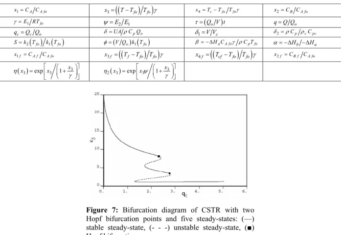
Torres and Tlacuahuac (2000) have analyzed input/output multiplicities of the full model using qc

as continuation parameter. In the bifurcation diagram of Figure 7, five steady-states and a bifurcation point were observed for x3 when qc=2.3.

Table 3: Dimensionless Parameters of the CSTR (Torres and Tlacuahuac, 2000).

1 A A fo

x =C C x₃=

(

(

T−T_fo

)

T_fo

)

γ x4=Tc−Tfo Tfoγ x2=CB CA fo 1 fo

E RT =

γ ψ=E E_{2 1} τ=(Q V to ) q=Q Qo

c c o

q =Q Q δ=UAρC Qp o δ1=V Vc δ2=ρCp ρcCpc

( ) ( )

2 fo 1 fo

S=k T k T φ=(V Q_o)k T₁

( )

_fo β= −ΔH Ca A foγ ρC Tp fo α= −ΔHb −ΔHa 1f A f A fo

x =C C x_3f =

(

(

T_f−T_fo

)

T_fo

)

γ x_4f=

(

(

T_cf−T_fo

)

T_fo

)

γ x2f =CB f CA fo

( ) 3 3 exp 3 1

x x = ⎡_⎢x ⎛_⎜ + ⎞_⎟⎤_⎥

⎝ ⎠

⎣ ⎦

η

γ 2( )3 exp 3 1 3

x x = ⎡_⎢x ⎛_⎜ + ⎞_⎟⎤_⎥

⎝ ⎠

⎣ ⎦

η ψ

γ

The CSTR model parameter values used for generating Figure 7 are shown in Table 4.

Table 4: CSTR Model Parameter Values (Torres and Tlacuahuac, 2000).

Ф δ q α S ψ δ1 δ2 x1f x2f x3f x4f

8 0.133 1 1 1 0.01 1 10 1 1000 1 0 0 -1

We define the state and measurements to be:

[

1 2 3 4

]

T

x= x x x x (57)

[

1 2

]

T

y= x x (58)

[

]

0 0.01 2 8 6

T

x = (59)

We consider state estimators with the following parameters:

2 0 0.05 4 4x

P = I (60)

1 0.1

k k

t t t ₋

Δ = − = (61)

(

2 2

)

0.0001 0.001

R=diag (62)

2 0 0.001 4 4

Q = I _× (63)

[

]

T

0 0.11 0.3 6 4

x = (64)

RESULTS AND ANALYSES

In this section we analyze the state estimator performances considering the operating region in which five steady-states and a Hopf bifurcation point were observed for x3 when qc=2.3 (cf. Figure 7). Comparison Between Unconstrained EKF For-mulations

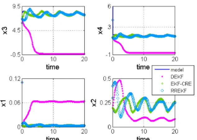
The poor initial guess x₀ given by Eq. (64) was selected because it leads DEKF to converge to an undesirable steady-state. In the absence of any meas-urement noise perturbation, RREKF and EKF-CRE were also applied to the CSTR. As shown in Figure 8, both unconstrained formulations converged to the actual steady-state, which in fact is a limit cycle. Likewise for the first example, RREKF presents a

slower convergence to the actual steady-state when compared to EKF-CRE.

Figure 8: Comparison between DEKF, EKF-CRE and RREKF performances for a system tending to multiple steady-states.

As mentioned before, RREKF disregards non-dominant eigenvectors. For this example, we use a rank-one approximation and three non-dominant eigenvectors were eliminated:

-1 -5

1, _{-1 -1}

6.9199 10 6.6802 10

-2.1715 10 6.8848 10

T

eq

υ = ⎢⎡ × × ⎤⎥

× ×

⎢ ⎥

⎣ ⎦

-1 -3

2, _{-1 -1}

-7.1769 10 3.9471 10

-3.0988 10 -6.2360 10

T

eq

υ = ⎢⎡ × × ⎤⎥

× ×

⎢ ⎥

⎣ ⎦

-2 -2

3, _{-1 -1}

7.7967 10 1.6892 10

-9.2549 10 -3.7027 10

T

eq

υ = ⎢⎡ × × ⎤⎥

× ×

⎢ ⎥

⎣ ⎦

At the equilibrium point x_eq=

[

0.0038 0.2649

]

7.6441 1.6208T, we observe that the eigenvectors 1,eq

υ υ_2,eq and υ_3,eq are bi-orthogonal to the tangent of the equilibrium curve (the scalar product is

negative). These three eigenvectors are not

considered in the rank-one covariance approximation and thus the filter applies no correction in their directions.

Therefore, the RREKF applies correction only in the

dominant eigenvector direction: -3

4,eq 1.4697 10

υ =⎡_⎣ ×

-1 -2 -3

State Estimation of Chemical Engineering Systems Tending to Multiple Solutions 783 Again, the state covariance matrix computed by

EKF-CRE in a single stage presents a smaller condi-tion number than the state covariance matrices com-puted by DEKF, as shown in Figure 9.

Figure 9: Comparison between the condition number of DEKF and EKF-CRE state covariance matrices for a system tending to multiple steady-states.

Comparison Between Clipped DEKF and CEKF

We have constrained DEKF with an ad hoc clipping strategy in order to prevent an undesirable steady-state. Nonetheless, the strategy of resetting to zero the negative update values did not perform well for this example and the clipped DEKF converged to the same undesirable steady-state as for the DEKF (cf. Figure 8). Thus, we selected stricter constraints for update values of the estimated states x3 and x4:

if xˆ₃< 5, set xˆ₃= 5 if xˆ₄< 0, set xˆ₄= 1.5

The strategy of resetting to zero the negative update values was maintained for the measured states x1 and x2.

The comparison between clipped DEKF and CEKF performances are shown in Figure 10.

Although both formulations swiftly converged to the actual states, the CEKF performed slightly better than the clipped DEKF for the CSTR case, as shown in Figure 10.

Finally, we also enlarged the MHE estimation window to N=2 for the CSTR case. In addition, the state covariance matrix of MHE was computed recursively using either the discrete Riccati equation (MHE-DRE) (Eq. (31) or the continuous Riccati equation (MHE-CRE) (Eq. (26) applied to each horizon step). The comparison between the CEKF,

MHE with DRE (N=2) and MHE (N=2) with CRE performances is shown in Figure 11.

Figure 10: Comparison between clipped DEKF and CEKF performances for a system tending to multiple steady-states until t=2.

Figure 11: Comparison between CEKF, MHE using DRE (N=2) and MHE (N=2) with CRE performances for a system tending to multiple steady-states until

t=2.

According to Figure 11, MHE is superior to CEKF to swiftly converge to the actual states. Since CRE is not subject to errors due to model discretiza-tion, it is not surprising that MHE-CRE presents more accurate estimates of states.

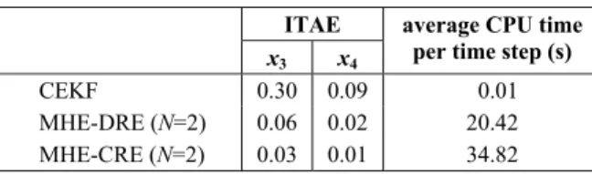
MHE-DRE and around 90% considering a size horizon of 2 in MHE-CRE. However, the improvement of esti-mation when MHE is implemented is reflected in a higher computational effort: 3 orders of magnitude larger.

Table 5: Comparison between CEKF and MHE-DRE and MHE-CRE: ITAE and Computational Expenses.

ITAE x3 x4

average CPU time per time step (s)

CEKF 0.30 0.09 0.01 MHE-DRE (N=2) 0.06 0.02 20.42 MHE-CRE (N=2) 0.03 0.01 34.82

In the case study reference (Torres and Tlacuahuac, 2000), the variables are dimensionless and nothing is said about the original units. However, in order to estimate the non-measured states, we suppose a sam-pling time of 0.1. If this value were in hours, which is proper to obtain concentrations measurements, both CEKF and MHE are suited for this case study.

It has been seen that MHE provides improved state estimation and presents greater robustness to a poor guess of the initial state. However, after con-verging to the actual states, both MHE and CEKF perform equally accurately and, therefore, the use of MHE becomes needless for the systems studied in this work.

In practice, however, chemical engineering sys-tems are frequently subject to unexpected process disturbances. Because MHE employs a trajectory of measurements during the state estimation, it shall present a better performance when compared to CEKF to handle with such problem.

CONCLUSION

This paper outlines the performance of the state covariance matrices used in three unconstrained Ex-tended Kalman Filter (EKF) formulations and one constrained EKF formulation (CEKF), for two chemical engineering examples tending to multiple solutions.

The first example is a batch reactor with reversi-ble reactions whose system model and measurement are such that multiple states satisfy the equilibrium condition. With a measurement noise perturbation, we outline a condition that led a classical EKF for-mulation (DEKF) to converge to physically unrealiz-able or undesired states. According to our results, EKF-CRE and RREKF are more numerically robust

in computing the state covariance matrix than DEKF. As both formulations avoided an increase in error propagation due to a measurement noise perturba-tion, they were able to converge to the actual steady-state. Thus, a suitable choice of the EKF formulation based on the state covariance matrix equation is es-sential to prevent physically unrealizable states. However, due to the poor guesses of the initial state and its state covariance matrix for the batch reactor, EKF-CRE and RREKF did not prevent physically unrealizable states during the batch. The clipped DEKF has been seen as a reasonable alternative to prevent physically unrealizable states, although this approach converges slowly to the actual states and disregards the assumption that the measurement noise is a Gaussian random noise and that clipped state estimates violate the process model. On the other hand, the CEKF can be seen as the best tech-nique for systems with such behavior due to the pos-sibility of incorporating constraints into an optimiza-tion problem minimizing the noise in a least square sense, preventing bad noise distribution. Besides, it is simpler, computationally less demanding than the MHE, and has comparable performance.

The second example is a CSTR with exothermic irreversible reactions and cooling jacket, whose nonlinear behavior includes multiple steady-states and limit cycles. The results for the CSTR demon-strate that, similar to the batch reactor case, EKF-CRE and RREKF converged to the actual steady-state. However, the clipped DEKF and CEKF pre-sented faster convergence to the actual states, and the CEKF performed slightly better than the clipped DEKF for this example. Contrary to the batch reac-tor, MHE presented a superior performance for the CSTR case. Further, we demonstrated that MHE performs better when the state covariance matrix is computed recursively using the continuous-time Riccati equation.

State Estimation of Chemical Engineering Systems Tending to Multiple Solutions 785

ACKNOWLEDGMENT

We gratefully acknowledge Prof. James Rawlings and Prof. Fernando Lima for the fruitful discussions. The first author also would like to thank the financial support from the German Academic Exchange Ser-vice (DAAD) and from PETROBRAS S.A.

REFERENCES

Brown, R. G. and Hwang, P. Y. C., Introduction to Random Signals and Applied Kalman Filtering: With MATLAB Exercises and Solutions, 4th Edition. John Wiley & Sons, New York (2012). Cox, H., On the estimation of state variables and

parameters for noisy dynamic systems. IEEE Transactions on Automatic Control, 9(1), 5-12 (1964).

Gesthuisen, R., Klatt, K. -U., Engell, S., Optimiza-tion-based State Estimation: A comparative study for the batch polycondensation. European Control Conference (ECC) (2001).

Grewal, M. S. and Andrews, A. P., Kalman Filtering: Theory and Practice Using MatLab, 3rd Edition, John Wiley & Sons, New Jersey (2008).

Haseltine, E. L. and Rawlings, J. B., Critical evalua-tion of extended Kalman filtering and moving-ho-rizon estimation. Ind. Eng. Chem. Res., 44, 2451-2460 (2005).

Jazwinski, A. H., Stochastic Processes and Filtering Theory. Academic Press, New York (1970). Kalman, R., Canonical structure of linear

dynami-cal systems. Proc. Natl. Acad. Sci., 48, 596-600 (1962).

Muske, K. R. and Rawlings, J. B., Nonlinear moving horizon state estimation, methods of model based process control. NATO ASI Series, 293, 349-365 (1994).

Petzold, L. R., DASSL: Differential Algebraic Sys-tem Solver. Technical Report of Sandia National Laboratories. Livermore (1983).

Pham, D. T., Verron, J. and Roubaud, M. C., A Sin-gular evolutive extended Kalman filter for data assimilation in oceanography. Journal of Marine Systems, 16(3-4), 323-340 (1998).

Prakash, J., Patwardhan, S. C. and Shah, S. L., Con-strained nonlinear state estimation using ensemble

Kalman filters. Ind. Eng. Chem. Res., 49, 2242-2253 (2010).

Rao, C. V., Rawlings, J. B., Constrained process monitoring - moving horizon approach. AIChE Journal, 48(1), 97-109 (2002).

Rao, C. V., Rawlings, J. B. and Mayne, D. Q., Con-strained state estimation for nonlinear discrete-time systems: Stability and moving horizon ap-proximations. IEEE Transactions on Automatic Control, 48(2), 246-258, (2003).

Robertson, D. G., Lee, J. H. and Rawlings, J. B., A moving horizon-based approach for least-squares estimation. AIChE Journal, 42(8), 2209-2224 (1996).

Salau, N. P. G., Trierweiler, J. O. and Secchi, A. R., Numerical pitfalls by state covariance computa-tion. Computer Aided Chemical Engineering, 27, 1215-1220 (2009).

Salau, N. P. G., Trierweiler, J. O. and Secchi, A. R., Observability analysis and model formulation for nonlinear state estimation. Accepted for Publica-tion in Applied Mathematical Modeling (2013). Secchi, A. R., Morari, M., Biscaia Jr., E. C., DAWRS:

A Differential - Algebraic System Solver by the Waveform Relaxation Method. The Sixth Distrib-uted Memory Computing Conference (DMCC6), Portland (1991).

Simon, D., Optimal State Estimation: Kalman, H-infinity, and Nonlinear Approaches. John Wiley & Sons, New Jersey (2006).

Tenny, M. J. and Rawlings, J. B., Efficient moving horizon estimation and nonlinear model predic-tive control. American Control Conference, An-chorage (2002).

Torres, A. E. G. and Tlacuahuac, A. F., Effect of process modeling on the nonlinear behaviour of a CSTR reactions AÆBÆC. Chemical Engineering Journal, 77, 153-164 (2000).

Vachhani, P., Narasimhan, S. and Rengaswamy, R., Recursive state estimation in nonlinear processes. American Control Conference, Boston (2004). Vachhani, P., Rengaswamy, R., Gangwal, V. and

Narasimhan S., Recursive estimation in con-strained nonlinear dynamical systems. AIChE Journal, 51(3), 946-959 (2005).