www.ocean-sci.net/12/481/2016/ doi:10.5194/os-12-481-2016
© Author(s) 2016. CC Attribution 3.0 License.
Compensation between meridional flow components
of the Atlantic MOC at 26
◦
N
E. Frajka-Williams1, C. S. Meinen2, W. E. Johns3, D. A. Smeed4, A. Duchez4, A. J. Lawrence1, D. A. Cuthbertson1, G. D. McCarthy4, H. L. Bryden1, M. O. Baringer2, B. I. Moat4, and D. Rayner4
1Ocean and Earth Science, University of Southampton, National Oceanography Centre Southampton, SO14 3ZH, UK 2Atlantic Oceanographic and Meteorological Laboratory, Physical Oceanography Division, 4301 Rickenbacker Causeway, Miami, FL 33149, USA
3University of Miami, Rosentiel School of Marine and Atmospheric Science, 4600 Rickenbacker Causeway, Miami, FL, USA 4National Oceanography Centre, University of Southampton Waterfront Campus, European Way, Southampton,
SO14 3ZH, UK
Correspondence to:E. Frajka-Williams ([email protected]) Received: 9 October 2015 – Published in Ocean Sci. Discuss.: 13 November 2015 Revised: 8 March 2016 – Accepted: 17 March 2016 – Published: 1 April 2016
Abstract. From ten years of observations of the Atlantic meridional overturning circulation (MOC) at 26◦N (2004– 2014), we revisit the question of flow compensation between components of the circulation. Contrasting with early results from the observations, transport variations of the Florida Current (FC) and upper mid-ocean (UMO) transports (top 1000 m east of the Bahamas) are now found to compensate on sub-annual timescales. The observed compensation be-tween the FC and UMO transports is associated with hori-zontal circulation and means that this part of the correlated variability does not project onto the MOC. A deep baroclinic response to wind-forcing (Ekman transport) is also found in the lower North Atlantic Deep Water (LNADW; 3000– 5000 m) transport. In contrast, co-variability between Ekman and the LNADW transports does contribute to overturning. On longer timescales, the southward UMO transport has con-tinued to strengthen, resulting in a concon-tinued decline of the MOC. Most of this interannual variability of the MOC can be traced to changes in isopycnal displacements on the west-ern boundary, within the top 1000 m and below 2000 m. Sub-stantial trends are observed in isopycnal displacements in the deep ocean, underscoring the importance of deep bound-ary measurements to capture the variability of the Atlantic MOC.
1 Introduction
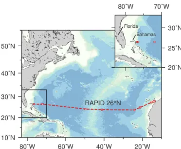
The Atlantic meridional overturning circulation (MOC) is a key part of the global ocean circulation, redistributing heat and properties around the globe. The continuous daily time-series observations at 26◦N (Fig. 1) are the first of their kind, capturing the transbasin circulation variability on timescales of days to – now – a decade.
Figure 1.Map of the study area. The RAPID array is shown with dashed lines crossing the Atlantic around 26◦N. Mooring positions are given by red squares. The inset is marked by the black rectangle, and shows a zoomed in view of the western boundary region.
been shown to be responsible for changes in ocean heat con-tent in the subtropical and tropical North Atlantic (Cunning-ham et al., 2014; Bryden et al., 2014).
Numerical investigations into the sources of variability to the Atlantic MOC interannual variability suggest that much of the variability may be attributable to winds (Cabanes et al., 2008; Roberts et al., 2013; Zhao and Johns, 2014; Yang, 2015; Pillar et al., 2016). Buoyancy forcing instead affects decadal variations (Polo et al., 2014; Yeager, 2015). An esti-mate of the MOC from high latitude density anomalies sug-gests a decline of the MOC (Robson et al., 2014), which is presently observed at 26◦N (observed trend of−0.5 Sv yr−1; Smeed et al., 2014) though it may not be indicative of a longer-term decline (Roberts et al., 2014). The 26◦N ar-ray provides an estimate of the MOC, but separating it into components and even depth ranges of anomalies may aid in the identification of physical causes of change (Wunsch and Heimbach, 2013).
In this paper, we introduce the 10-year record of the MOC at 26◦N, describing features of the variability in the most recent 18 months and across the 10-year record, and exam-ine more fully the degree of correlation or compensation between MOC components using the longer records. While much of the recent research into Atlantic MOC variability has focused on interannual timescales and longer, here we quantify newly observed compensation between the Florida Current and UMO transports, and co-variability between the deep transbasin transports and zonal winds, on sub-annual timescales. The depth structure and timescales of these vari-ations are explored, illustrating an important role for the western boundary below 1000 m. Lower-frequency changes in MOC components, including the continuing trend in the
vertical shear of the mid-ocean transport, are also described. Finally, we conclude by discussing the origins of the lower-frequency variability in the 10-year records.
2 Methods
The international 26◦N Rapid Climate Change (RAPID)/Meridional Overturning Circulation and Heat Flux Array (MOCHA), hereafter RAPID 26◦N, has pro-vided comprehensive daily measurements of the MOC at 26◦N for 10 years (April 2004–March 2014; Smeed et al., 2015). The MOC is defined as the northward transport above the depth of maximum overturning (roughly 1100 m) across 26◦N, and is constructed as the sum of three components: the surface meridional Ekman transport estimated from reanalysis winds, the Gulf Stream transport through the Florida Straits – the Florida Current (FC) – measured by a submarine cable (e.g. Meinen et al., 2010), and the upper mid-ocean (UMO) transport, measured by a transbasin array of current metre and dynamic height moorings between the Bahamas and Africa. The exact number of moorings and instruments has varied over the past decade during which there have been over 20 deployment and recovery cruises. The main western boundary mooring that we used here is called WB2, and typically has 18 MicroCAT (Seabird Electronics, Bellevue, WA) conductivity–temperature–depth instruments. Vertical resolution ranges from 75 m near the surface to 500 m near the bottom. Overall, the accuracy of the MOC transport is estimated to be 1.5 Sv (10-day values) or 0.9 Sv (annual averages). Full details of the array configuration and map (their Fig. 1.1), transport calculation, and associated errors can be found in McCarthy et al. (2015). Here, we focus on the transbasin or mid-ocean (MO) trans-port, from which the UMO is derived. The MO transport is constructed from three parts:
MO(z)=Twbw(z)+Tint(z)+Text(z), (1) where Twbw is the western boundary transport estimated from direct current metre measurements,Tint the “internal” transbasin transport, andTextthe “external” flow. The west-ern boundary wedge transport,Twbw, includes most of the flow associated with the Antilles Current. The internal trans-port, Tint, is the baroclinic flow zonally integrated across the remainder of the ocean interior relative to an assumed level of no motion at 4820 dbar. It is derived from dynamic height moorings near the western and eastern boundaries and over the Mid-Atlantic Ridge (Fig. 1). Here we focus on the western and eastern profile contributions to theTint. Using only the western and eastern density contributions to interior transport per unit depth,Tint(z)relative to the reference level (zref) is related to density as
Tint(z)= −
g
fρ
z
Z
zref
wheregis gravitational acceleration,f the Coriolis param-eter, andρe(z)andρw(z)the density profiles at the eastern and western boundary, respectively (Rayner et al., 2011).
The external flow, Text, is the (unmeasured) interior barotropic flow that ensures zero mass transport across the section. This component is calculated as a residual of the other components and is applied as a uniformly distributed, and thus depth-independent, velocity across the entire mid-ocean section, which we refer to as hypsometric compensa-tion. Due to changes in the width of the basin as a function of depth, even though the applied flow is barotropic, the trans-port per unit depth has decreasing magnitude with increasing depth. Kanzow et al. (2007) showed that this estimate – de-rived from mass conservation – was in good agreement with an independent estimate of the mid-ocean barotropic flow de-rived from bottom pressure gauges deployed across the sec-tion over the April 2004–April 2005 period.
The MO transport can be further divided into its contri-butions to the upper and lower branches of the overturn-ing circulation. The UMO is defined as the depth integral of MO transport between the surface and the time-varying depth of maximum overturning, roughly 1100 m. The lower limb of the MOC is made up of southward flowing North Atlantic Deep Water, which is split into contributions associ-ated with upper North Atlantic Deep Water (UNADW; 1100– 3000 m) and lower North Atlantic Deep Water (LNADW; 3000–5000 m). The sum of these two transports recovers nearly all the variability of the MOC (r=0.996; McCarthy et al., 2012). The small difference is equal to the flow be-tween 1100 m and the depth of maximum overturning and a contribution from the hypsometric compensation below 4820 bar.
For the analysis presented here, we start with the RAPID data as processed for the publicly available data set. This pro-cessing involves filtering individual instrument records with a 2-day low-pass filter to remove the tides, and subsampling onto 12-hourly intervals. From this subsampled data set, transport components are computed, then further 10-day low-pass filtered with a fifth-order Butterworth filter before the compensation transport is calculated (Kanzow et al., 2007). These data are available from http://www.rapid.ac.uk/. Here we additionally bin the data onto a twice-monthly time grid, then remove the twice-monthly climatology to reduce sea-sonal variations. For lower-frequency variations, deseasea-sonal- deseasonal-ized time series are further filtered with a 1.5 year Tukey fil-ter. Significance and confidence intervals are reported at the 95 % level, unless otherwise indicated. The number of de-grees of freedom was calculated using the integral timescale of decorrelation to the first zero crossing (Emery and Thom-son, 2004). When a year is denoted 2009/10, it refers to the period 1 April 2009 through 31 March 2010.
For the purpose of calculating isopycnal displacements
ζ, absolute salinities and conservative temperatures on the twice-monthly time grid are used. Isopycnal (σ) displace-ments are then calculated following Desaubies and Gregg
(1981), as
ζ (z(σ¯ i), t )=z(σi, t )− ¯z(σi) ,
using locally referenced densities. For example, to deter-mine the displacement of the isopycnal typically found at 1000 dbar, potential densities are calculated referenced to 1000 dbar (σ1). Using these locally referenced densities, the mean density at 1000 dbar is identified (σi= hσ1(z= 1000, t )it). The depth of this density, z(σi, t ), is then de-termined for each time step in the locally referenced den-sities, and differenced from its mean depth (∼991 m for 1000 dbar). This produces isopycnal displacements as a func-tion of density, which can then be mapped back onto depth using the mean relationship between depth and density (z(σ¯ i)). This process of locally referencing densities is re-peated for each pressure surface from the surface to the bot-tom at 20 dbar intervals. The detrended and low-pass filtered time series are processed as above.
3 10-years of MOC and mid-ocean variability
All of the 10-year time series of transport components at 26◦N show high-frequency variability (Fig. 2a). In the most recent 18 months, additional features of the time se-ries include a large Ekman transport reversal in March 2013 (similar to the two reversals that occurred in 2009/10 and 2010/11). During the March 2013 event, the Ekman transport anomalies exceeded 2 standard deviations from the mean, with the typically northward-flowing water turned to the south. This reversal was similar in magnitude to the De-cember 2009–March 2010 event, but with shorter duration (Fig. 2a). On several occasions, as during the negative Ek-man events in 2005, 2010, and 2013, the FC also showed sharp, short-term reductions in transport. These correspond-ing anomalies led to sharp reductions – or even brief reversals – of the MOC at these times. Over the past 10 years, the MOC was negative from 19 to 24 December 2009, and from 9 to 13 March 2013. The Ekman transport reversals also coincided with reductions of the southward LNADW flow (Fig. 2b). In the most recent 5 years, the LNADW experienced more short periods of reversal (i.e. a northward flow of the net transport below 3000 m) than had been observed in the first 5 years of the record. These high-frequency events in the deep flow exhibit fairly weak vertical shear, with maximum anomalies below 3000 m (Fig. 3a).
2004 2005 2006 2007 2008 2009 2010 2011 2012 2013 2014 -30
-20 -10 0 10 20 30 40
Transport [Sv]
(a) MOC & components FC MOC Ek UMO
2004 2005 2006 2007 2008 2009 2010 2011 2012 2013 2014 -20
-10 0 10
Transport [Sv]
(b) Deep mid–– ocean transports
LNADW UNADW
Figure 2. (a)Transport time series of the FC (blue), Ekman (green),
upper mid-ocean (magenta), and overturning (red) at 10-day reso-lution.(b)Layer transports for UNADW (1100–3000 m, cyan) and LNADW (3000–5000 m, purple). For visualization purposes, the fil-tered versions of the time series are shown in black, where trans-ports have been convolved with a 4-month, low-pass Hanning win-dow. Transports are positive northwards; 10-year mean transports for each components are shown with the dotted lines.
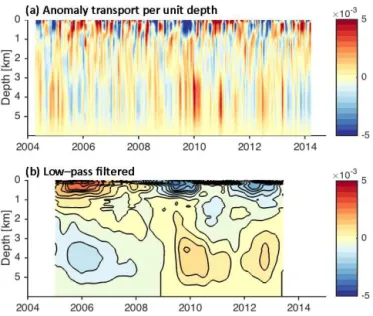
Figure 3. Transport-per-unit-depth anomalies of the mid-ocean
transport at 26◦N, where the time-mean profile over the 10 years has been removed.(a)The top panel shows the twice-monthly, de-seasonalized variability and(b)the lower panel is further filtered with the 1.5 year filter. Red (blue) shows transports that are anoma-lously northward (southward).
the southward thermocline flow (UMO) has persisted with the associated weakening of the MOC. The 2012/13 year was the second weakest year of the MOC (14.2 Sv), behind the 2009/10 year (12.8 Sv). In contrast to the 2009/10 year, the weak MOC in 2012/13 had very little contribution from the
Figure 4.Time series of transport anomaly for MOC and
compo-nents as in Fig. 2, deseasonalized and low-pass filtered with 1.5 year filter.
Table 1.Mean±standard deviation of transports for the first 5 years
and latter 5 years, where years run from 1 April–31 March. Standard deviations are calculated on the annual averages. Statistically signif-icant changes to the mean are indicated by bold, based on two-tailed ttests.
Component 2004–2009 2009–2014 Change
[Sv] [Sv] [Sv]
FC 31.7±0.2 31.0±0.3 −0.7
Ekman 3.7±0.4 3.4±1.0 −0.3
UMO −17.0±1.2 −18.8±1.0 −1.9
MOC 18.4±1.3 15.5±1.9 −2.9
UNADW −12.0±0.3 −11.8±0.7 0.2
LNADW −7.1±0.9 −4.7±1.5 2.3
wind-driven Ekman transport, but instead is associated with a strong southward thermocline flow (UMO).
Transport-per-unit depth anomaly profiles show the depth structure of mid-ocean transport variations. In the top 1100 m, the southward UMO has intensified (Fig. 3b, shift from red to blue), while below 3000 m the southward LNADW has weakened (shift from blue to red). Previous analyses have shown that variability of the UMO on inter-annual timescales is primarily governed by changes at the western boundary (Frajka-Williams, 2015). The amplitude of these changes is larger in the top 1000 m, but anomalies below 1000 m span a large portion of the water column.
4 Correlation between transport components
west-2004 2006 2008 2010 2012 2014 -10
-5 0 5
Trans. anom. [Sv]
(a) Detrended
-10 -5 0 5 -10
-5 0 5
FC
(b) r=0.49
2004 2006 2008 2010 2012 2014
-2 -1 0 1 2
Trans. anom. [Sv]
(c) Low–– pass filtered
UMO -FC
-2 -1 0 1 2
UMO
-2 -1 0 1 2
FC
(d) r=0.23
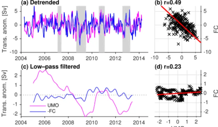
Figure 5.Transport anomaly time series (left column) for the−FC
(blue) and UMO (magenta). Zero anomaly is marked with the dashed line. Scatter plots of the same (right column) with correla-tion coefficients (r) noted. In(a, b), the deseasonalized, detrended time series are used. In(c, d), the time series are deseasonalized and low-pass filtered, but not detrended. The orthogonal regression line is overlaid on the scatter plots. Grey bars highlight periods noted in the text.
ern boundary: the FC and Antilles Current from 2009 to 2011, the end of the record at the time of publication (Frajka-Williams et al., 2013). From the 10-year record (2004–2014), we now see correlations emerging between some of the con-tributing terms, which has implications for how we under-stand the large-scale circulation at 26◦N. Considering the 3-month-filtered UMO and FC transport time series (black lines in Fig. 2), anomalies of opposite sign appear to coin-cide in late 2008, late 2010, and again in late 2012. Dur-ing the 2010/11 winter, for example, the northward flowDur-ing FC weakened by several Sverdrups. At the same time, the southward flowing UMO weakened by nearly 10 Sv. We in-vestigate these apparent compensations (between the UMO and FC, and also between LNADW and wind-driven Ekman flow) more rigorously in the following section.
4.1 UMO and FC transports: Horizontal circulation
The FC carries most of the waters of the Gulf Stream across 26◦N. The origins of this water come from the Yucatan Channel and Old Bahama Channel, across complex topogra-phy west of the Bahamas (Rousset and Beal, 2014). At simi-lar latitudes, the flow through the Yucatan Channel has been found to compensate flow around Cuba (Lin et al., 2009), while variations in the FC have, at times, shown compen-sation east of the Bahamas in bottom pressure variations (Bryden et al., 2009) and in top 1000 m velocities (Frajka-Williams et al., 2013).
Here we consider compensation between FC and UMO, the transbasin transport east of the Bahamas. This compensa-tion can be clearly seen by plotting their detrended anomaly time series (Fig. 5a). Certain events stand out, demonstrat-ing almost perfect correspondence between the two time
se-ries, with examples including February–May 2007, Septem-ber 2008–June 2009, August 2010–January 2011 and August 2012–March 2013 (highlighted in the figure). Notably, these episodes of correlation are absent in the first 3 years. The overall correlation between the two records is r= −0.49, significant at the 95 % level.
Fluctuations in UMO compensate fluctuations in the FC by similar magnitudes (slope= −0.92, Fig. 5b). When the northward FC transport increases along the western bound-ary, the southward UMO transport east of the Bahamas in-tensifies by the same amount. This means that excess north-ward flow in the boundary current is returned horizontally within the upper mid-ocean circulation rather than by deeper layers in the interior, which would have involved changes in the MOC. The region east of the Bahamas is known to be rich with eddies, which may influence the transbasin trans-ports (Wunsch, 2008; Kanzow et al., 2009; Thomas and Zhai, 2013; Clément et al., 2014; Xu et al., 2014), and due to the timescale of observed compensation, we suspect that eddies are involved.
Using the low-pass filtered time series, this high degree of compensation is absent (Fig. 5c and d). Instead, strong inter-annual variability in the UMO remains (Fig. 5c). By compari-son, the low-pass filtered FC shows little interannual variabil-ity, consistent with previous work that indicated that the in-terannual and longer period FC variability is of much smaller amplitude than the sub-annual variability (e.g. DiNezio et al., 2009; Meinen et al., 2010). While the two time series are not significantly correlated (r=0.24), both show a reduc-tion from the first 5-year period (April 2004–March 2009) to the latter 5-year period (April 2009–March 2014; see also Table 1), with the FC reducing by 0.7 Sv and the UMO by 1.9 Sv. Unlike the compensation at higher frequencies, these changes are both of the same sign (note that the negative of UMO is plotted in Fig. 5a), compounding the effect on the MOC (net reduction of 2.9 Sv).
4.2 LNADW and Ekman transports: deep wind-driven
response
2004 2006 2008 2010 2012 2014
Trans. anom. [Sv]-10
-5 0 5
(a) Detrended
-10 -5 0 5
Ekman
-10 -5 0 5
(b) r=0.58
2004 2006 2008 2010 2012 2014
Trans. anom. [Sv] -2
-1 0 1 2
(c) Low–– pass filtered
Ekman -LNADW
LNADW
-2 -1 0 1 2
Ekman
-2 -1 0 1 2
(d) r=0.51
Figure 6. As Fig. 5 but for the Ekman and−LNADW transport
anomaly time series.
As with the FC and UMO compensation, magnitudes of fluctuations between Ekman and LNADW match (slope= −0.84, with Ekman anomalies of 1 Sv corresponding to a 0.84 Sv change in the LNADW). Unlike the FC and UMO, however, the correlation between the LNADW and Ekman at higher frequencies projects onto the MOC rather than can-celling. This is consistent with expectations that the high-frequency, wind-driven variability of Ekman transport results in an overturning, albeit a shallow one (where the depth of overturning is at the base of the northward Ekman trans-port) between the surface Ekman transport and return flow below (Jayne and Marotzke, 2001; Killworth, 2008). Varia-tions in Ekman or FC project directly on the mid-ocean trans-port (through theTextterm in 2), and bottom pressure records at the western boundary also covary with Ekman anomalies (McCarthy et al., 2012). However, we will show that the co-variations between FC, Ekman, and mid-ocean transports are not limited to theTextcontribution, but are instead associated with density changes at the western boundary.
To identify possible lags between the UMO and FC or Ek-man and LNADW, we use the 10-day filtered time series. For both correlations, between the UMO and FC and between the Ekman and LNADW, the timescale of the response is fast (Fig. 7). For the LNADW and Ekman correlation, a maxi-mum correlation ofr=0.51 is found at 1-day lag with Ek-man leading. This means that the wind response occurs es-sentially instantaneously. For the UMO and FC transports, a maximum correlation ofr=0.46 is found for UMO lead-ing by 0.5 days. This lead–lag relationship can also be seen by inspecting close-zoomed plots of the time series during large anomalies (Fig. 7e). Due to filtering applied to individ-ual instrument data and transport time series, such a short lag is not statistically meaningful.
Aug Sep Oct Nov
Trans. anom. [Sv] -5
0 5 10
15(a) Aug–– Nov 2010
-FC UMO
Sep Oct Nov Dec -5
0 5 10
15(b) Sep–– Dec 2012
Dec Jan Feb Mar
Trans. anom. [Sv]-15
-10 -5 0 5
(c) Dec–– Mar 2010
-LNADW Ekman
Feb Mar Apr May Jun -15
-10 -5 0 5
(d) Feb–– Jun 2013
MO lags - MO leads [days]
-30 -20 -10 0 10
Corr. coeff.
-0.5
-0.4
-0.3
-0.2
(e) Lag correlation
Figure 7.10-day filtered transport anomaly time series of UMO
and FC(a, b)and LNADW and Ekman(c, d). The 10-year mean has been removed, but the seasonal cycle and trends are retained. Time ranges have been chosen to correspond to large anomalies in both time series, to visualize possible lags.(e)Lag correlation between 10-day filtered UMO and FC (magenta), and Ekman and LNADW (green); 95 % significance is marked by the dashed lines, same colour.
5 Depth structure of co-variability
The hypsometric compensation term (Text) is mostly depth-independent, but has a vertical profile that scales with the width of the basin as a function of depth. It is nearly uni-form from the surface to about 3500 m, and then decreases gradually to zero at the greatest depths in the basin. If the mid-ocean region had no shear (Tint=0) and no flow in the wedge (Twbw=0), the MO transport would still be non-zero through this applied compensation, in order to balance the northward FC and Ekman transport. In the absence of strong variations in Tint, we would expect to see anti-correlation between the MO transports (e.g. the UMO and LNADW) and the independently estimated FC and Ekman transports. In this case, the MO transport fluctuations would then have a depth structure approximately matching the hypsomet-ric profile. Instead, the MO transport-per-unit-depth profiles often show deep maxima below 3500 m in anomaly plots (Fig. 3a).
a constant depth at the eastern boundary, the shear would be controlled by displacements at the western boundary.
While the stratification at 26◦N is more continuous, we use displacements at the two basin boundaries to investi-gate the magnitude of the shear variability and the role of east and west in producing these shear anomalies. Using the time-mean density gradient profile, given by N2(z)= −(g/ρ)∂ρ/∂z¯ , the contribution of heave to transport per unit depth can be estimated from Eq. (2) as
e
Tint(z)= 1
f
z
Z
zzref ζeNe
2
−ζwNw 2
dz′, (3)
where∼distinguishes this portion ofTintfrom the more com-plete calculation in Eq. (2). Here,ζe(z, t )andζw(z, t )are the isopycnal displacements at the east and west, respectively. From Eq. (3), we might expect some correspondence be-tween isopycnal displacements and transports, though trans-ports are the vertically integrated transport per unit depth.
Comparing the UMO transport with both eastern and west-ern boundary isopycnal displacement time series, we find strong correlations (Fig. 8a). In the west, displacements be-tween 300 and 1200 m are significantly correlated with the UMO time series, with a peak at 820 m. This is consistent with physical expectations, and prior results indicated a role for the displacement of the main thermocline in controlling the UMO transport (Longworth et al., 2011; McCarthy et al., 2012; Duchez et al., 2014). The correlation in the east is of similar absolute amplitude but is spread over a broader depth range (200 to ∼1800 m deep), consistent with the findings of Chidichimo et al. (2010) that the eastern boundary den-sity variations were coherent down to 1400 m. No significant correlations were found between any of the transport compo-nents considered here (UMO, FC, LNADW, or Ekman) and the isopycnal displacements at the Mid-Atlantic Ridge (not shown).
The FC is also highly correlated with the western bound-ary thermocline displacement (Fig. 8a). The sign of the corre-lation has flipped, consistent with the anti-correcorre-lation noted between the FC and UMO. This relationship is statistically significant, even though the isotherms covarying with the FC are 150 km away from the FC, east of the Bahamas. As might be expected, there is no statistically significant relationship between the thermocline displacements on the eastern side of the basin and the FC transport. Comparing the time se-ries of western boundary isopycnal displacements at 820 m with the UMO transport (Fig. 9a), we find significant corre-lation where a 10 m downward displacement of the thermo-cline corresponds to a 1 Sv increase in the UMO transport (Fig. 9b). Given the one-to-one relationship between the FC and UMO (Fig. 5b), this means that a 10 m thermocline dis-placement is also associated with a 1 Sv change in the FC.
The correlation between LNADW transport and isopyc-nal displacements is significant at depth (1500 m–bottom) on
-1 -0.5 0 0.5 1
Corr. coeff.
0
1
2
3
4
5
Depth [km]
(a) UMO, FC
-1 -0.5 0 0.5 1
Corr. coeff. (b) LNADW, Ekman
Figure 8. Correlation between isopycnal displacements at each
depth and transport time series, where time series are deseason-alized and detrended. (a) Correlation between UMO (magenta) and isopycnal displacements at the west (solid) and east (dashed), and between FC (blue) and isopycnal displacements at the west (solid) and east (dashed). Significant correlations are indicated by the thicker line.(b)The same, but for LNADW (purple) and Ekman (green).
Figure 9.Time series of deseasonalized, detrended transports and
isopycnal depths.(a)UMO transport (magenta) and the depth of the density surface with mean position at 820 m (highest correla-tion with UMO) at the west.(c)LNADW transport (purple) and the depth of the density surface with highest correlation (at 3140 m). Scatter plots are shown in(b, d), where the least-squares linear re-gression is overlaid.
thousand metres of water (spanning several moored instru-ments), so that when water at 3000 m moves upwards, a large segment of the water column above and below is also mov-ing upwards (though with differmov-ing magnitudes). In this case, a 42 m downward displacement of the isopycnal at 3140 m results in a 1 Sv reduction in the LNADW transport (Fig. 9d). Isopycnal displacements in a reduced region (2700– 3300 m) at the western boundary are also significantly cor-related with the surface Ekman transport (Fig. 8b). Positive (northward) Ekman transport anomalies are associated with upward displacements of the deep isopycnals. This means that when the winds blow along 26◦N, the deep ocean re-sponds by heaving upwards or downwards across hundreds of metres, with the end result that these isopycnal displace-ments at the western boundary change the basin-wide tilt and thus the vertical shear in meridional transports. Just 40 km offshore (25 km further offshore than the western boundary) at the WB3 mooring, isopycnal displacements are still significantly correlated with LNADW transports, albeit more weakly (|r| ≤0.5, not shown). Ekman transports are no longer correlated with displacements. At the WB5 mooring, 500 km offshore, there is no relationship between isopycnal displacements and basin-wide transport. The strong correla-tion between isopycnal displacements nearshore and merid-ional Ekman transport, and the absence of correlation for off-shore displacements may indicate that the deep compensa-tion is concentrated at the western boundary, or that other variability in isopycnal displacements masks the signal off-shore.
6 Timescales of compensation/co-variability
One of the key results presented here is that the UMO and FC transports often compensate each other – i.e. their signs dif-fer but anomalies match – resulting in greatly reduced impact of their individual fluctuations on the total MOC variabil-ity. However, this compensation is dependent on timescales. At low-frequencies, the compensation does not dominate (Fig. 5c), and the large interannual variability and trend in the UMO transport has a strong projection onto the interan-nual variability and trend of the MOC.
To investigate the co-variability for different timescales, we evaluate the coherence calculated using a multitaper spec-trum following Percival and Walden (1998) (Fig. 10). The FC and UMO are significantly coherent and out-of-phase (i.e. anti-correlated) at periods less than 1 year. For periods longer than about a year they are no longer coherent. For Ekman and LNADW transports, they are coherent at periods shorter than 900 days (except near 120 days) and also (nearly) out-of-phase. By contrast, there is little coherence between the Ekman and FC time series (Fig. 10, grey).
These results at first appear to contradict Kanzow et al. (2010), who noted from the first 3 years of observations (2004–2007) that there was no compensation between the FC
Period
30 d 90 d .5 yr 1 yr 2 yr 4 yr
Coherence [
γ
2 ]
0 0.2 0.4 0.6 0.8 1
(a) Coherence
FC:UMO LNADW:Ek FC:Ek
Period
30 d 90 d .5 yr 1 yr 2 yr 4 yr
χ
[degrees]
-90 0 90 180
(b) Phase
Figure 10.Coherence between MOC components: UMO and FC
(magenta), LNADW and Ekman (green) and FC and Ekman (grey), where time series are the original 10-day filtered (seasonal varia-tions retained). The top panel shows coherence, where significance is delimited by the black horizontal line. The lower panel shows the phase relationship at each period in degrees.
Figure 11. (a)Cross-wavelet transform between the FC and UMO shows high power (red) with a fixed-phase relationship since 2007 at periods between 60 and 400 days.(b)Cross-wavelet transform between Ekman and LNADW shows high power primarily at annual periods during the 2009–2010 events, as well as sub-annual from 50–150 days in 2005, 2011, and 2013. (Arrows pointing to the left indicate out-of-phase relationship or anti-correlation, and are only shown when the relationship is significant. Deviations from 180◦ indicate a lag or phase shift.)
the AC, as long as the AC is geostrophic. The mooring used to estimate isopycnal displacements is at the western edge of the UMO transport, but is east of the core of the north-ward AC velocities. This means that a downnorth-ward displace-ment of isopycnals is associated with an increase in the tilt of the thermocline between Africa and the mooring, but will have an opposing effect on geostrophic transports west of the mooring, in the Antilles Current. Frajka-Williams et al. (2013) identified stronger eddy activity east of the Bahamas during the period of FC and AC correlation, which is consis-tent with a eddy activity playing a role in the anti-correlation between the FC and UMO on subannual timescales.
7 Trends in isopycnal displacements and MO transports
The MOC at 26◦N has been decreasing in strength, as de-scribed in Smeed et al. (2014) and this trend continues through early 2014. This low-frequency change is mainly as-sociated with changes in the UMO transport (variations at timescales longer than 1 year) and to a lesser degree with a weak reduction in the FC transport (Table 1). From the low-pass filtered transport-per-unit depth profiles (Fig. 3b), we noted that changes are present both above and below the thermocline. Here we investigate how the trends in transport are captured by trends in isopycnal displacements.
In the top 1000 m, the isopycnal slope is large, with lighter water in the west. The slope decreases to 0 at about 1000 m, reversing sign between 1000–1500 m, and is typi-cally small below (Fig. 12a). At the western boundary, isopy-cnal displacements below 1000 m are moving downwards (trend at 3140 m is−6.5±3.5 m yr−1, increasing to about
−13±0.4 m yr−1 at 4500 m), while above 500 m they are moving upwards (Fig. 12b). At the eastern boundary, trends are near zero except below 4000 m where they are down-ward. As a result, the east–west slope of isopycnals below 1000 m is decreasing with time. While the largest displace-ments are seen at depth, stratification is also weaker at depth. From Eq. (3), we see that the effect of isopycnal displace-ments on transports is modulated by the background stratifi-cation. Computing instead the trends in isopycnal displace-ments scaled by stratification (Fig. 12c), we now see that at the western boundary, the effect of isopycnal displacements below the thermocline is nearly constant, with little effect on the eastern boundary. Scaling by stratification emphasizes the importance of relatively small trends in displacements in the top 1000 m to transport anomalies.
The trend inTeint from Eq. (3) is shown in Fig. 12d, with a persistent reducing trend in the interior transports associ-ated with heave at the eastern and western boundaries. The magnitude of the trend increases from 0 at the bottom, since it is integrated upwards from the bottom. While the ther-mocline displacement shows little-to-no trend (Fig. 12b, the trend on the western boundary at 830 m is−0.7±0.9 m yr−1), the interior transport has a large negative trend. The large am-plitude at the depth of the thermocline results from the accu-mulation of persistent negative anomalies between the bot-tom and the thermocline. Above 1000 m, the trend inTeint(z) is relatively constant and negative.
A southward intensification ofTint, if unbalanced by other components, would result in an overall intensification of the southward flow across the section over the 10-year period. To maintain overall mass balance across the section, an oppos-ing trend is required inText(Fig. 12e). Trends in the overall mid-ocean transport (MO(z)) include those fromeTintas well as anomalies in the wedge and compensation, due to stratifi-cation changes and diabatic changes, and both at the bound-aries and Mid-Atlantic Ridge. The overall amplitude of the trend in MO(z)is weaker than ineTint(z), but with a greater shear near the surface. The wedge in particular contributes to the shear in the top 1000 m in MO(z)relative toeTint(not shown).
-50 0 50 150 East minus West [m]
0
1
2
3
4
5
Depth [km]
(a) Mean tilt
-30 -20 -10 0 10 Rate [m yr ] 0
1
2
3
4
5
b) ( ζ trends
West East Std
-10 0 10 20 Rate [m yr ] 0
1
2
3
4
5
(c) dζ/dt(N/N )0
-8 -6 -4 -2 0 2
[1x10 Sv m yr ]-4 -1
0
1
2
3
4
5
(d) Tint
Tint MO-Text
-8 -6 -4 -2 0 2
[1x10 Sv m yr ]-4 -1
0
1
2
3
4
5
(e) Transport
MO T
ext
MO-Text
~
-1 -1 -1 -1
Figure 12.Trend in isopycnal displacements and transports.(a)Mean height difference between isopycnals in the east and west.(b)Trend
in isopycnal displacements at the western and eastern boundaries, where a negative (positive) trend indicates downward (upward) movement of isopycnals. The solid (dashed) line is for displacements at the west (east).(c)Trend in displacements scaled by buoyancy frequency with N0=1×10⁻³s−1.(d)Trend ineTintfrom Eq. (2). The red line is the trend in MO(z)−Text.(e)Trends in transport per unit depth of
mid-ocean (MO(z)) in magenta,Textin blue. All time series were twice monthly. Confidence intervals on the trends are shaded. The dotted line
shows a zero trend.
southward flow. In addition, the depth of the change in the trend (1700 m) is in the middle of the UNADW layer (1100– 3000 m) offering an explanation for why no long-term trend is apparent in the UNADW transport.
8 Discussion
Here we have identified significant compensation, dependent on timescale, between components of the MOC: for exam-ple, on sub-annual timescales when the FC is stronger north-ward in the western boundary, the UMO compensates with stronger southward flow between the Bahamas and Canary islands. While these components are largely independent, they are weakly coupled due to the construction of the MO(z)
transports. The Text term contributes variability to both the UMO and LNADW transport, and would tend to cause an opposite sign anomaly in both the UMO and LNADW in re-sponse to anomalies in the FC and Ekman transports.
However, by construction the Text term is nearly barotropic, and what limited vertical structure it has arises from the vertical profile of section width at 26◦N. This means that Text distributes compensation for the Ekman or FC anomalies across the full water column, with the strongest compensation in the MO(z)term occurring in the top 3500 m and reducing to zero at the bottom. Only a fraction of FC anomalies (order one-fifth) would be projected byTextonto UMO anomalies, and less than half the magnitude of Ekman anomalies would be contained in the LNADW portion of the
Text. Instead, the observed transport anomalies in UMO and
LNADW are indistinguishable in magnitude to the anomalies in FC and Ekman transports. Furthermore, there is no cor-relation between the Ekman and UNADW transport, which requires a shear between LNADW and UNADW to remove any projected compensation to Ekman. We can see this baro-clinic response in the isopycnal displacements measured at the western boundary.
The relationship between surface winds and deep isopyc-nal displacements is harder to understand, and we presently do not have a dynamical explanation for this behaviour. Nevertheless, the observations are quite clear: when there is anomalous southward Ekman transport (resulting from westerly winds), isopycnals at ∼3000 m on the western boundary plunge downwards. From theoretical and numer-ical model results (Jayne and Marotzke, 2001; Killworth, 2008), it is expected that Ekman transport fluctuations on sub-annual timescales should result in a quasi-instantaneous, and nearly barotropic, compensation in the deep ocean. One might expect that with anomalous southward Ekman trans-port across the basin, there should be a northward compen-sation across a broad range of depths, which could also per-haps be spatially distributed. Yeager (2015) showed in a nu-merical model that Ekman anomalies project strongly onto the barotropic mode promoting wave interactions with deep bathymetry. It is possible that the baroclinic response we ob-serve at 26◦N is generated by these barotropic waves inter-acting with the bathymetry at the western boundary. This is an area for future research – likely requiring numerical mod-elling to isolate mechanisms and processes.
The observed high-degree of variability on sub-annual timescales of the UMO and LNADW transports may con-tribute to the apparent absence of meridional coherence be-tween observations at 26◦N and higher latitudes. Elipot et al. (2013) found large coherence on short timescales at mid-latitudes in the North Atlantic, but between 41 and 26◦N, transport anomalies were out-of-phase (Elipot et al., 2014; Mielke et al., 2013). The large fluctuations in LNADW trans-port are remarkably well captured by ocean bottom pressure from the GRACE satellites (Landerer et al., 2015). How-ever, the spatial footprint of detrended monthly anomalies is centred in the western part of the subtropical North At-lantic, suggesting limited meridional coherence. Using satel-lite altimetry, Frajka-Williams (2015) found that sea surface height anomalies capture the interannual variability and trend of the UMO transport, with a spatial footprint extending over a larger area.
9 Conclusions
The record of basin-wide MOC transport variability at 26◦N in the Atlantic is now 10-years long. It continues to deliver new insights into the origins of the changing large-scale cir-culation at 26◦N. In this paper, we have provided a brief overview of the latest 18 months of observations. In particu-lar, with the most recent 18 months of observations, the April 2012 to March 2013 year has the second weakest MOC, be-hind the 2009/10 year. Unlike the 2009/10 year, the reduction in 2012/13 is associated with an enhanced southward UMO and decreased LNADW, with no contribution from anoma-lous Ekman transport. There were, however, several wind-reversal events in the latest 18 months, at the end of 2012
and again in March 2013. These events were shorter than the 2009/10 and 2010/11 double dip, though they also resulted in concurrent reductions in the southward LNADW transport.
The main result of this paper has been detailing newly identified compensations between MOC components (UMO and FC, and LNADW and Ekman). Using the 10-year record, we now find that on shorter timescales (periods shorter than 1 year), much of the variability of the UMO is compensated by the FC transport variability, particularly in the most recent 7 years. On similar timescales (periods shorter than 2 years), the wind-driven variability in the top 100 m (surface merid-ional Ekman transport) is nearly instantaneously balanced by deep flow in the opposite direction. However, rather than be-ing a simple barotropic response to the winds, the imprint of the winds is baroclinic, with the strongest signature in isopy-cnal displacements being found just east of the Bahamas at 3000 m depth.
There is a key difference between these two compensat-ing transport pairs. Between the FC and UMO, compen-sated high-frequency transport anomalies results in a hori-zontal circulation anomaly: that is, northward flow in the FC (in the top 700 m) is accompanied by southward flow in the top 1100 m east of the Bahamas. As a consequence, trans-port anomalies have little influence on the MOC and are un-likely to have a strong heat transport anomaly. By contrast, the southward Ekman anomalies accompanied by northward LNADW anomalies directly projects onto the MOC. During the anomalous periods of exceptionally strong (weak) Ekman transport, the MOC is similarly strong (weak) and we expect the meridional heat transport to vary with the MOC (Johns et al., 2011).
Finally, investigating longer-term variations of the MOC, we can localize the origin of the intensifying trend in the MOC to isopycnal displacements on the western boundary. Observed transport fluctuations on interannual and longer timescales present a different story. From the 10-year record, the mid-ocean transports (rather than FC and Ekman) are primarily responsible for the low-frequency variability and trend of the overturning. Furthermore, the trend in trans-port variability is associated with the persistent deepening of isopycnals below the thermocline at the western boundary. These displacements are greatest in the abyss (130±40 m over 10 years at 4500 m) compared to about 60±30 m at mid-depths around 2000 m, though their impact on transports must be scaled by stratification. While we do not investigate here whether the longer-term isopycnal deepening is asso-ciated with water mass changes or wind-forcing, a coinci-dent shift towards warmer and fresher waters below 3000 m (Atkinson et al., 2012) hints at the possibility of larger-scale persistent changes to the Atlantic circulation.
funded by the Natural Environment Research Council (NERC), National Science Foundation (NSF, OCE1332978) and National Oceanic and Atmospheric Administration (NOAA), the Climate Program Office – Climate Observation Division. Data are freely available from www.rapid.ac.uk.
Florida Current transports are funded by the NOAA and are avail-able from www.aoml.noaa.gov/phod/floridacurrent.
Wavelet code provided by A. Grinsted, J. Moore and S. Jevre-jeva. Special thanks to the captains, crews, and technicians, who have been invaluable in the measurement of the MOC at 26◦N over the past 10 years.
Edited by: M. Hoppema
References
Atkinson, C. P., Bryden, H. L., Cunningham, S. A., and King, B. A.: Atlantic transport variability at 25◦N in six hydrographic sec-tions, Ocean Sci., 8, 497–523, doi:10.5194/os-8-497-2012, 2012. Bryden, H. L., Longworth, H. R., and Cunningham, S. A.: Slow-ing of the Atlantic meridional overturnSlow-ing circulation at 25◦N, Nature, 438, 655–657, 2005.
Bryden, H. L., Mujahid, A., Cunningham, S. A., and Kanzow, T.: Adjustment of the basin-scale circulation at 26◦N to variations in Gulf Stream, deep western boundary current and Ekman trans-ports as observed by the Rapid array, Ocean Sci., 5, 421–433, doi:10.5194/os-5-421-2009, 2009.
Bryden, H. L., King, B. A., McCarthy, G. D., and McDonagh, E. L.: Impact of a 30 % reduction in Atlantic meridional overturning during 2009–2010, Ocean Sci., 10, 683–691, doi:10.5194/os-10-683-2014, 2014.
Cabanes, C., Lee, T., and Fu, L.-L.: Mechanisms of inter-annual variations of the Meridional Overturning Circula-tion of the North Atlantic, J. Phys. Ocean., 38, 467–480, doi:10.1175/2007JPO3726.1, 2008.
Chidichimo, M. P., Kanzow, T., Cunningham, S. A., Johns, W. E., and Marotzke, J.: The contribution of eastern-boundary density variations to the Atlantic meridional overturning circulation at 26.5◦N, Ocean Sci., 6, 475–490, doi:10.5194/os-6-475-2010, 2010.
Clément, L., Frajka-Williams, E., Szuts, Z. B., and Cunning-ham, S. A.: The vertical structure of eddies and Rossby waves and their effect on the Atlantic MOC at 26◦N, J. Geophys. Res., 119, 6479–6498, doi:10.1002/2014JC010146, 2014.
Cunningham, S. A., Kanzow, T., Rayner, D., Baringer, M. O., Johns, W. E., Marotzke, J., Longworth, H. R., Grant, E. M., Hirschi, J. J.-M., Beal, L. M., Meinen, C. S., and Bryden, H. L.: Temporal variability of the Atlantic meridional overturning cir-culation at 26.5◦N, Science, 317, 935–938, 2007.
Cunningham, S. A., Roberts, C., Frajka-Williams, E., Johns, W. E., Hobbs, W., Palmer, M. D., Rayner, D., Smeed, D. A., and McCarthy, G. D.: Atlantic MOC slowdown cooled the subtropical ocean, Geophys. Res. Lett., 40, 6202–6207, doi:10.1002/2013GL058464, 2014.
Desaubies, Y. and Gregg, M. C.: Reversible and irreversible finestructure, J. Phys. Ocean., 11, 541–556, 1981.
DiNezio, P. N., Gramer, L. J., Johns, W. E., Meinen, C. S., and Baringer, M. O.: Observed interannual variability of the Florida
Current: Wind forcing and the North Atlantic Oscillation, J. Phys. Oceanogr., 39, 721–736, 2009.
Duchez, A., Frajka-Williams, E., Castro, N., Hirschi, J. J.-M., and Coward, A.: Seasonal to interannual variability in density around the Canary Islands and their influence on the AMOC at 26.5◦N, J. Geophys. Res., 119, 1843–1860, doi:10.1002/2013JC009416, 2014.
Elipot, S., Hughes, C., Olhede, S., and Toole, J.: Coherence of western boundary pressure at the RAPID WAVE array: Bound-ary wave adjustments or deep western boundBound-ary current advec-tion?, J. Phys. Oceanogr., 43, 744–765, 2013.
Elipot, S., Frajka-Williams, E., Hughes, C., and Willis, J.: The observed North Atlantic MOC, its meridional coherence and ocean bottom pressure, J. Phys. Oceanogr., 44, 517–537, doi:10.1175/JPO-D-13-026.1, 2014.
Emery, W. J. and Thomson, R. E.: Data Analysis Methods in Phys-ical Oceanography, Elsevier, Amsterdam, the Netherlands, 2nd edn., 2004.
Frajka-Williams, E.: Estimating the Atlantic MOC at 26◦N using satellite altimetry and cable measurements, Geophys. Res. Lett., 42, 3458–3464, doi:10.1002/2015GL063220, 2015.
Frajka-Williams, E., Johns, W. E., Meinen, C. S., Beal, L. M., and Cunningham, S. A.: Eddy impacts on the Florida Current, Geo-phys. Res. Lett., 40, 349–353, doi:10.1002/grl.50115, 2013. Grinsted, A., Moore, J. C., and Jevrejeva, S.: Application of the
cross wavelet transform and wavelet coherence to geophys-ical time series, Nonlin. Processes Geophys., 11, 561–566, doi:10.5194/npg-11-561-2004, 2004.
Jayne, S. R. and Marotzke, J.: The dynamics of ocean heat transport variability, Rev. Geophys., 39, 385–411, 2001.
Johns, W. E., Baringer, M. O., Beal, L. M., Cunningham, S. A., Kanzow, T., Bryden, H. L., Hirschi, J. J.-M., Marotzke, J., Meinen, C. S., Shaw, B., and Curry, R.: Continuous, array-based estimates of Atlantic Ocean heat transport at 26.5◦N, J. Climate, 24, 2429–2449, 2011.
Kanzow, T., Cunningham, S. A., Rayner, D., Hirschi, J. J.-M., Johns, W. E., Baringer, M. O., Bryden, H. L., Beal, L. M., Meinen, C. S., and Marotzke, J.: Observed flow compensation as-sociated with the MOC at 26.5◦N in the Atlantic, Science, 317, 938–941, 2007.
Kanzow, T., Johnson, H. L., Marshall, D. P., Cunningham, S. A., Hirschi, J. J.-M., Mujahid, A., Bryden, H. L., and Johns, W. E.: Basinwide Integrated Volume Transports in an Eddy-Filled Ocean, J. Phys. Oceanogr., 39, 3091–3110, 2009.
Kanzow, T., Cunningham, S. A., Johns, W. E., Hirschi, J. J.-M., Marotzke, J., Baringer, M. O., Meinen, C. S., Chidichimo, M. P., Atkinson, C., Beal, L. M., Bryden, H. L., and Collins, J.: Seasonal variability of the Atlantic meridional overturn-ing circulation at 26.5◦N, J. Climate, 23, 5678–5698, doi:10.1175/2010JCLI3389.1, 2010.
Killworth, P. D.: A simple linear model of the depth dependence of the wind-driven variability of the Meridional Overturning Circu-lation, J. Phys. Oceanogr., 38, 492–502, 2008.
Lin, Y., Greatbatch, R. J., and Sheng, J.: A model study of the vertically integrated transport variability through the Yu-catan Channel: Role of Loop Current evolution and flow compensation around Cuba, J. Geophys. Res., 114, C08003, doi:10.1029/2008JC005199, 2009.
Longworth, H. R., Bryden, H. L., and Baringer, M. O.: Histor-ical variability in Atlantic meridional baroclinic transport at 26.5◦N from boundary dynamic height observations, Deep-Sea Res. Pt. II, 58, 1754–1767, 2011.
McCarthy, G., Frajka-Williams, E., Johns, W. E., Baringer, M. O., Meinen, C. S., Bryden, H. L., Rayner, D., Duchez, A., Roberts, C. D., and Cunningham, S. A.: Observed interannual variability of the Atlantic MOC at 26.5◦N, Geophys. Res. Lett., 39, L19609, doi:10.1029/2012GL052933, 2012.
McCarthy, G. D., Smeed, D. A., Johns, W. E., Frajka-Williams, E., Moat, B. I., Rayner, D., Baringer, M. O., Meinen, C. S., and Bryden, H. L.: Measuring the Atlantic meridional over-turning circulation at 26◦N, Prog. Oceanogr., 130, 91–111, doi:10.1016/j.pocean.2014.10.006, 2015.
Meinen, C. S., Baringer, M. O., and Garcia, R. F.: Florida Current transport variability: An analysis of annual and longer-period sig-nals, Deep-Sea Res. Pt. I, 57, 835–846, 2010.
Mielke, C., Frajka-Williams, E., and Baehr, J.: Observed and sim-ulated variability of the AMOC at 26◦N and 41◦N, Geophys. Res. Lett., 40, 1159–1164, doi:10.1002/grl.50233, 2013. Percival, D. B. and Walden, A. T.: Spectral Analysis for
Physi-cal Applications, Cambridge University Press, Cambridge, UK, 1998.
Pillar, H., Heimbach, P., Johnson, H., and Marshall, D.: Dynamical attribution of recent variability in Atlantic overturning, J. Cli-mate, doi:10.1175/JCLI-D-15-0727.1, 2016.
Polo, I., Robson, J., Sutton, R., and Bamaseda, M.: The importance of wind and buoyancy forcing of the boundary density variations and the geostrophic component of the AMOC at 26◦N, J. Phys. Oceanogr., 44, 2387–2408, 2014.
Rayner, D., Hirschi, J. J.-M., Kanzow, T., Johns, W. E., Wright, P. G., Frajka-Williams, E., Bryden, H. L., Meinen, C. S., Baringer, M. O., Marotzke, J., Beal, L. M., and Cun-ningham, S. A.: Monitoring the Atlantic meridional over-turning circulation, Deep-Sea Res. Pt. II, 58, 1744–1753, doi:10.1016/j.dsr2.2010.10.056, 2011.
Roberts, C. D., Waters, J., Peterson, K. A., Palmer, M., Mc-Carthy, G. D., Frajka-Williams, E., Haines, K., Lea, D. J., Mar-tin, M. J., Storkey, D., Blockley, E. W., and Zuo, H.: Atmosphere drives observed interannual variability of the Atlantic merid-ional overturning circulation at 26.5◦N, Geophys. Res. Lett., 40, 5164–5170, doi:10.1002/grl.50930, 2013.
Roberts, C. D., Jackson, L., and McNeall, D.: Is the 2004– 2012 reduction of the Atlantic meridional overturning cir-culation significant?, Geophys. Res. Lett., 41, 3204–3210, doi:10.1002/2014GL059473, 2014.
Robson, J., Hodson, D., Hawkins, E., and Sutton, R.: Atlantic over-turning in decline?, Nat. Geosci., 7, 2–3, doi:10.1038/ngeo2050, 2014.
Rousset, C. and Beal, L. M.: Closing the transport budget of the Florida Straits, Geophys. Res. Lett., 41, 2460–2466, doi:10.1002/2014GL059498, 2014.
Smeed, D. A., McCarthy, G. D., Cunningham, S. A., Frajka-Williams, E., Rayner, D., Johns, W. E., Meinen, C. S., Baringer, M. O., Moat, B. I., Duchez, A., and Bryden, H. L.: Observed decline of the Atlantic meridional overturning circulation 2004– 2012, Ocean Sci., 10, 29–38, doi:10.5194/os-10-29-2014, 2014. Smeed, D. A., McCarthy, G., Rayner, D., Moat, B. I., Johns, W. E., Baringer, M. O., and Meinen, C. S.: At-lantic meridional overturning circulation observed by the RAPID-MOCHA-WBTS (RAPID-Meridional Overturning Circulation and Heatflux Array-Western Boundary Time Series) array at 26◦N from 2004 to 2014, available at: https://www.bodc.ac.uk/data/published_data_library/catalogue/ 10.5285/1a774e53-7383-2e9a-e053-6c86abc0d8c7/, last access: 15 August 2015.
Thomas, M. D. and Zhai, X.: Eddy-induced variability of the merid-ional overturning circulation in a model of the North Atlantic, Geophys. Res. Lett., 40, 2742–2747, doi:10.1002/grl.50532, 2013.
Wunsch, C.: Mass and volume transport variability in an eddy-filled ocean, Nat. Geosci., 1, 165–168, doi:10.1038/ngeo126, 2008. Wunsch, C. and Heimbach, P.: Two decades of the Atlantic
merid-ional overturning circulation: Anatomy, variations, extremes, prediction, and overcoming its limitations, J. Climate, 26, 7167– 7186, doi:10.1175/JCLI-D-12-00478.1, 2013.
Xu, X., Chassignet, E. P., Johns, W. E., Schmitz Jr., W. J., and Metzger, E. J.: Intraseasonal to interannual variability of the Atlantic meridional overturning circulation from eddy-resolving simulations and observations, J. Geophys. Res., 119, 5140–5159, doi:10.1002/2014JC009994, 2014.
Yang, J.: Local and remote wind stress forcing of the seasonal variability of the Atlantic Meridional Overturning Circulation (AMOC) transport at 26.5◦N, J. Geophys. Res., 120, 2488– 2503, doi:10.1002/2014JC010317, 2015.
Yeager, S.: Topographic coupling of the Atlantic overturning and gyre circulations, J. Phys. Oceanogr., 45, 1258–1284, doi:10.1175/JPO-D-14-0100.1, 2015.