Module Management Tool in Software Development Organizations

(1)

ISSN 1549-3636

Corresponding Author: Ahmad A. Al-Rababah, Faculty of IT, Al-Ahliyyah Amman University, P.O. Box 252,19328, Amman, Jordan

Module Management Tool in Software Development Organizations

1_{Ahmad A. Al-Rababah and}2_{Mohammad A. Al-Rababah}

1_{Faculty of IT, Al-Ahliyyah Amman University, P.O.Box 252,19328, Amman, Jordan}

2_{Faculty of Science, Jerash Private University, Jordan}

Abstract: Module management is an important task at developers’ level in software development organizations. So we consider in this paper software as collection of several modules. Also we study a method of clustering of modules of a large software system. The need of doing such clustering is justified to be an important part of software management in the software development organizations. An algorithm of maintenance and modifications is presented for doing the clustering by the developers in the respective development organizations, whose complexity is calculated. The method will be very much helpful, as an essential tool, at the developer level in software development organizations for module management.

Key words: Link graphs, link matrix, MC, updated link matrix, coupling matrix

INTRODUCTION

The software architect devotes best effort for deriving an overall structural model of the system as a collection of several modules[1], as far as possible by retaining loose links. This helps the developers to modify the modules almost independently, irrespective of the codes of other modules. But in reality, it is not always feasible to develop any system as a collection of only mutually independent modules. Module management[2-4] is a very important job at the developers surface to improve the process visibility and the overall cost effectiveness. In object oriented model, modules are objects with private state and defined operations on that states. In the data flow models, modules are functional transformations. In both cases, module may be implemented as sequential components or as processes. An object-oriented model of a system architecture structures the system into a set of loosely coupled objects with well-defined interface [5,6].

Modules and link graphs: Among these modules, a pair of modules may be mutually independent (ideal situation), or may have link. If a flow of data (or a flow of control) exists between these two modules, we say that they are linked, they are not independent. Thus, there are three types of link possible to be existing between a pair of modules:

* mo link, (if the modules are mutually independent) * one link, (if there exists a flow of data or control

from any one module to other, but not both ways).

* two links (if there exists a flow of data or control both ways).

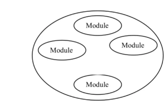
Module

Module Module

Module

Fig. 1: Software

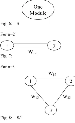
We ignore the trivial case of the existence of link of one module with itself. Thus, between a pair of modules, there could be at most two links (according to our concept of link as stated above). Consider a system S constituted of n modules developed under object oriented paradigm. Suppose that the modules are numbered from 1 to n. Consider two modules module-i and module-j.

i

j

(2)

Fig. 3: and

Fig.4: One-link graphs (directed)

Fig. 5: Two-link graph (directed)

Let us assume that any two modules are linked with some weight W (number of links) such that

Wij = weight of the link between module-i and

module-j Then,

Wij = 0, if no link

= 1, if one link = 2, if two links.

Clearly, Wij is commutative with respect to its indices i

and j. i.e. Wij = Wji.

Then the link graph of the system S will be an undirected graph as shown bellow:

For n=1

Fig. 6: S

For n=2

Fig. 7:

For n=3

W13

W12

W23

1 2

3

Fig. 8: W

For n=4

W23

W13 W24

W34 W14

W12

1 2

3 4

Fig. 9: and so on.

Link matrix and the integer set Zr: Now, let us divide each element Wij into two parts such that

* Wij = lij + lji ,

* lij = 1, if module-i has to send a deliverable to

module-j

= 0, if module-i will not have to send any deliverable to module-j. (and same type of definition is also true for every lij, i≠j).

We assume that lii =

D

or0

(don’t care symbol), (or the number 0) ignoring the cases of deliverables which are internal only. Obviously, mij and mji are not

necessarily equal. They are one way link values only. Then the Link matrix of the system S is defined as the square matrix L = [lij]

In the link matrix L, each row could be viewed as the modules to perform the role of suppliers and each column could be viewed as modules to perform the role of consumers.

Example of a link matrix: Consider a system S with 4 modules 1, 2, 3 and 4

   

 

   

  =

0 1 0 0

1 0 0 1

0 1 0 0

0 1 1 0

4 3 2 1

4 3 2 1 L

In this link matrix, the data l23 = 1 means that the

module-2 will send a deliverable to module-3, whereas the data l32 = 0 means that module-3 will not. The data

l14 =0 and l41= 0 combined signifies that module-1 and

module-4 are mutually independent, because W14 will

be zero in this case. If numbers of 1’s are more in the matrix L, it implies that there are many modules linked with each other. The ideal situation under object oriented paradigm is that the number of 0’s in non-diagonal positions of L should be more and more.

i

j

i

j

One

Module

W

12

1

2

(3)

Fig. 10: Link-graph of S (Undirected)

1 2

3 4

Fig. 11: Link-graph of S (Directed)

Integer-Set Zr: Let +

∈

I

r

. We define integer-set Zr as

the set of all non negative integer less than or equal to r. Thus, Z2= {0, 1, 2}, Z5= {0, 1, 2, 3, 4, 5} etc.

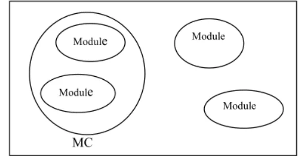
Clustering of modules: By grouping together the modules which interact with each other very closely, it’s certainly possible to reduce the efforts in the software maintenance[3,7]. Two or more closely related modules, if grouped as one object, forms a module-cluster (MC).

MC Module

Module

Fig. 12: Software system

Now, we study how to group two modules to form a cluster and then how to update the link-matrix of the system after completing each clustering. Consider the system S as chosen in example earlier.

Suppose that we like to group module-1 and module-2 to form a new cluster MC.

Module-1

Module-2

Fig. 13: One Cluster C1

For this we consider the sub matrix L1 of L

corresponding to row-1, row-2 and column-1, column-2 given by

L1 =

     

0 0

1 0

2 1

Now this new cluster C1 is to be treated as good as

one bigger module, say module-1 (specified by bold one). Thus, at present the system S consists of one cluster (the new created module-1), module-3 and module-4. The total number of deliverables from this cluster to module-i, (for i=2, 3) is clearly equal to the sum of the numbers of deliverables from module-1 and module-2 to module-i. The link values will now be changed accordingly, and thus our updated link-matrix for the system S will be as below:

L =

  

 

  

 

0 1 0

1 0 1

0 2 1

3 2 1

It’s to be noticed that in this updated link matrix L, l11 is not zero but 1, which is clear from the submatrix

L1, and the updated link matrix L is still a square

matrix. Also in the initial link matrix L of the system S, the matrix-elements

∈

Z1. In the first updated link

matrix L, the elements

∈

Z2. We will see next that in

the pth updated link matrix L of the system S, the

elements

∈

Zp+k where k

≥

1. Thus, after this

clustering, the software system S will be apparently as shown in Fig. 13 to the developers’ eyes. The method could be generalized to group together two clusters to form a bigger cluster of clusters. For example, the following two figures can be seen:

* New cluster (by grouping one cluster and one module)

Cluster _Module

Fig. 14: Cluster

2

1

2

0

1

2

3

4

(4)

* New cluster (by grouping two clusters)

Cluster _Cluster

Fig. 15: Cluster

Couplingmatrix M: Each module could be viewed as a trivial cluster initially. However, if we consider two clusters Cr and Cs, then these are two parameters which

we shall consider now. The parameters are:

* maximum number (m) of possible links between Cr

and Cs

* actual number (a) of links existing between Cr and

Cs

Clearly, the ratio 

    

m a

will be a member in the closed interval [0, 1]. This number (collectively for every pair of clusters) constitutes the coupling matrix M of a system S. For example, at the initial stage of the system S when each cluster contains exactly one module, the number a

∈

Z2 and m =2.

Thus, _

    

m

a

_∈

_{{0, ½, 1}. The elements of the}

coupling matrix MC= [mij] are defined now as below.

(There are three different cases):

Case 1: Suppose that both of the clusters contains single module only.

MC Ci MC Cj

Fig. 16:

In this case, a = wij = lij+lji and m = 2 where lij, lji

are elements of the current link matrix L of the system S.

Thus,

2

ji ij ij

ij

w

l

m

=

+

Clearly, mij

∈

[0, 1].

Case 2: Suppose that a cluster Ci contains ni number of

modules and another cluster Cj contains only one

module module-j.

In this case, mij =

,

2

i ji ij

n

l

+

because m = 2ni here.

Clearly mij

∈

[0,1].

Module

Module-j

MC Ci MC Cj

Fig. 17: Modules

Case 3: Suppose that a cluster Ci contains ni number of

modules and another cluster Cj contains nj number of

modules.

MC Cj MC Ci

Fig. 18: MCCi

In this case, m = 2ninj, and mij =

,

2 n

i

n

j

l

ij

+

ji

Where lij and lji are the elements of the last updated

link matrix of the software system S. In this case also, mij

∈

[0, 1]. Clearly, the coupling matrix M is a square

and a symmetric matrix. If mij =0, it indicates that the

two clusters Ci and Cj are mutually independent. If mij

is a low value, it indicates that the two clusters Ci and

Cj are loosely coupled and if it’s a high value (close to

1) then it indicates that the two clusters are strongly coupling. At every stage we shall look at the coupling matrix M to watch which pair of clusters is most strongly coupling and in the next step we will group these two clusters to form a new cluster. This is the main paradigm of clustering in our work here. Such pair of clusters is called Strongly Coupled Clusters (SCC).

The task of clustering by this method is continued until we reach at a single cluster (which is equivalent to the complete software system S). But it’s most preferable to stop once a small number of meaningful and low-coupling clusters have been reached upon.The final number of clusters should be optimal in the context of maintenance and modifications to be done by the developers in the respective development organizations. We shall not cluster Ci and Cj into one

cluster if mij = 0, or very close to zero. For this the

Developers (or the Software Development

(5)

Organization) choose a threshold value

µ

which is very close to zero. Now, we present an algorithm for the above task of clustering.

Algorithm for module clustering: Here, we present an algorithm for module clustering which is an improved version of the existing algorithms[7]. At each iteration in this algorithm, two clusters with strongest coupling-value are merged to form a new cluster and the link matrix is updated immediately. Since the coupling matrix M is a symmetric matrix, the elements of its uppers triangular region are sufficient for us to consider. The algorithm uses an important data structure which is an array N = < N1, N2, …, Nn > of n

elements, where Ni is number of modules present in the

ith cluster.

Clearly, at the initial stage, Ni = 1,

∀

i = 1 , 2, 3,……,n. Module-clustering Algorithm

Step 1: Calculate the initial link matrix L and the upper triangular portion of the coupling matrix M, (i.e.

∀

i and

∀

j where 1

≤

i

≤

j

≤

n)

Step 2: Repeat step-3 through step-6, (n-1) times.

Step 3: Find the pair of SCC with coupling value more than

µ

. (if more than one pair exists, chose any one arbitrarily) which are Ci’ and

Cj’

where 1

≤

i’

≤

j’

≤

n (this inequality which can be assumed with no loss of generality). Calculate mi’j’ = max {mij}, 1

≤

i

≤

j

≤

n

Step 4: Merge Ci’ and Cj’ to form a new cluster Ci’. Step 4.1: Ni’

←

Ni’ + Nj’

Step 4.2: Update ith column (ith row ) of the link

matrix such that

∀

k=1, 2, …n where, k

≠

i’,j’

li’k

←

li’k + lik

li’k

←

0

Step 5: Ignore now the cluster j’, and set Nji

←

0. Step 6: Update the coupling matrix M.

Step 6.1: Update the i’th row of M by doing:

∀

k=1, 2, …n

where k

≠

i’

mkj’

←

mki’

Step 6.2: Update i’th column of M by doing:

∀

k=1, 2, …n

where k

≠

i’

mj’k

←

mi’k Step 7: Stop.

Complexity of the algorithm: To calculate the complexity T(n) of the module clustering algorithm we see that:

In step-1, there will be computation of nC2 elements of

the coupling matrix M. The complexity of this step is O(n2)

Step-3 involves a sorting algorithm, in worst-case which will consume O(n2) amount of time (in case the developers seeks alternative SCC from the sorted clusters). All other steps from 4 to 6 have the complexity O(n) respectively. Thus, the portion from step-3 through step-6 has the complexity = O(n2) + O(n) = O(n2).

But, due to the repetition of this computation for (n-1) times ( because of step 2), we have the total complexity of the algorithm given by

T(n) = O(n2) + (n-1) * O(n2) = O(n3)

Thus, we see that the algorithm is a P-class algorithm.

CONCLUSION

We have studied here a methodology for module clustering in a huge type of software system which has been developed with a large number of modules. The need of doing such clustering is justified to be an important part of software management in the software development organizations. We present a polynomial time algorithm for module clustering and the method can be well applicable especially for the large software systems developed with object oriented approach. The final number of clusters should be optimal in the context of maintenance and modifications to be done by the developers in the respective development organizations.

REFERENCES

1. Gao, J.Z. and H.S.J. Tsao, 2006. Testing and Quality Assurance for Component-Based Software. Artech House Publishers.

2. Berczuk, S. and B. Appleton, 2002. Software Configuration Management Patterns: Effective Teamwork. Addison-Wesley.

3. Pullum, L.L., 2001. Software Fault Tolerance Techniques and Implementation, Norwood, MA: Artech House.

4. Summerville, I., 2002. Software Engineering, Pearson Education Asia. New Delhi.

5. Kartashev, S., 1990. Supercomputing Systems: Architectures, Design and Performance. New York.

6. Zedan, H.S.M. and A. Cau, 1999. Object-Oriented Technology and Computing Systems Re-Engineering. Horwood Publishing Limited.