Comparações quantitativas entre o sensor Hartmann-Shack e o sensor de
Castro e resultados preliminares para um olho mecânico
Trabalho desenvolvido no Instituto de Física de São Carlos - Universidade de São Paulo - USP - São Carlos (SP) Brazil; Universidade Federal de São Paulo -UNIFESP - São Paulo (SP) - Brazil.
1Instituto de Física de São Carlos - Universidade de São Paulo - USP - São Carlos (SP) - Brazil.
2Oftalmologista pela Universidade Federal de São Paulo - UNIFESP - São Paulo (SP) - Brazil.
3Oftalmologista pela UNIFESP - São Paulo (SP) - Brazil. 4Instituto de Física de São Carlos - USP - São Carlos
(SP) - Brazil.
Endereço para correspondência: E-mail: [email protected]
Recebido para publicação em 01.08.2005 Versão revisada recebida em 19.11.2005 Aprovação em 21.01.2006
Nota Editorial: Depois de concluída a análise do artigo sob sigilo editorial e com a anuência dos Drs. Paulo André Polisuk e Renato Ambrósio Jr. sobre a divulgação de seus nomes como revisores, agradece-mos sua participação neste processo.
Luis Alberto Carvalho1
Wallace Chamon2
Paulo Schor3
Jarbas Caiado de Castro4
Keywords: Diagnostic techniques, ophthalmological; Refractive errors/surgery
sensors and preliminary results for defocus aberrations
on a mechanical eye
Purpose: There is a general acceptance among the scientific community
of Cartesian symmetry wavefront sensors (such as the Hartmann-Shack (HS) sensor) as a standard in the field of optics and vision science. In this study it is shown that sensors of different symmetries and/or configurations should also be tested and analyzed in order to quantify and compare their effectiveness when applied to visual optics. Three types of wave-aberration sensors were developed and tested here. Each sensor has a very different configuration and/or symmetry (dodecagonal (DOD), cylindrical (CYL) and conventional Hartmann-Shack (HS)). Methods: All sensors were designed and developed in the Physics Department of the Universidade de São Paulo – São Carlos. Each sensor was mounted on a laboratory optical bench used in a previous study. A commercial mechanical eye was used as control. This mechanical eye has a rotating mechanism that allows the retinal plane to be positioned at different axial distances. Ten different defocus aberrations were generated: 5 cases of myopia from -1D to -5D and 5 cases of hyperopia, from +1D to +5D, in steps of 1D following the scale printed on the mechanical eye. For each wavefront sensor a specific image-processing and fitting algorithm was implemented. For all three cases, the wavefront information was fit using the first 36 VSIA standard Zernike polynomials. Results for the mechanical eye were also compared to the absolute Zernike surface generated from coefficients associated with the theoretical sphere-cylinder aberration value. Results: Precision was ana-lyzed using two different methods: first, a theoretical approach was used by generating synthetic Zernike coefficients from the known sphere-cylinder aberrations, simply by applying sphere-sphere-cylinder equations in the backward direction. Then comparisons were made of these coefficients with the ones obtained in practice. Results for DOD, HS and CYL sensors were, respectively, as follows: mean of root mean square (RMSE) for all aberrations, when theoretical Zernike coefficients were used as control, was 0.22, 0.66 and 0.26 microns; RMSE of sphere-cylinder values when compared to autorefractor measurements was 0.18D, 0.22D and 0.35D for sphere, 0.14D, 0.24D and 0.17D for cylinder, 34.36°, 35.16° and 26.36° for axis; RMSE of sphere-cylinder values when theoretical values were used as control was 0.11D, 0.29D and 0.46D for sphere, 0.15D, 0.28D and 0.17D for cylinder, 19.71°, 25.56° and 18.56° for axis. Conclusion: The main conclusion is that the symmetry of an optical sensor is not an important consideration when measuring typical eye aberrations such as defocus (myopic and hyperopic), but there are differences. In this sense, the polar symmetry sensors render results that are equivalent to the traditional Cartesian Hartmann-Shack sensor, but furnish an easier method for deter-mining the optical center.
240 Quantitative comparison of different-shaped wavefront sensors and preliminary results for defocus aberrations on a mechanical eye
INTRODUCTION
The interest in measuring optical aberrations of the eye dates many centuries(1). The Christian Jesuit Scheiner in the
year 1619 published the work entitled “Oculus, sive funda-mentum optikum”(2). In this work he demonstrated what
beca-me known years later and up to our days as the Scheiner Disc(2). The Scheiner disc consists of a small circular disc with
a peripheral and a central pinhole. Depending on the number and position of points seen by the patient when illuminated with a distant light source it was possible to infer if the patient was myopic, hyperopic or emmetropic.
After Scheiner’s Disc many other inventors and resear-chers introduced interesting methods for eye aberration diag-nosis. Tscherning in 1884(3) used a 4D spherical lens with a
grid pattern on its surface to project a regular pattern at the retina. He would then ask the patient to sketch drawings of the pattern. Depending on the pattern distortions Tscherning could have a semiquantitative measurement of the patient’s aberrations. It was only in the beginning of the 1960s that Howlland et al.(4) devised a quantitative version of the
Tscher-ning Aberroscope, by attaching an imaging system and imple-menting rigorous mathematical analysis of the collected data. Almost 300 years after Scheiner’s invention, Hartmann(5)
pro-posed an innovative method for measuring optical aberrations of general optical instruments and lenses. Hartmann’s idea was similar to the Tscherning mask but instead of a mask he used a grid pattern superimposed on a lens; he proposed a mask with a series of pinholes and a photographic film behind it. In this configuration a plane wavefront would form a perfect distribution of points over the photographic film and a distor-ted wavefront would form a distordistor-ted pattern, distribudistor-ted non-symmetrically. By applying a concept based on Hartmann’s idea, Shack proposed in 1971 that instead of pinholes a set of microlenses is used as “mask” and behind it a CCD camera instead of a photographic camera(6). Because of the
superpo-sition and concatenation of improvements, this sensor beca-me popularly known as the Hartmann-Shack (HS) sensor (or Shack-Hartmann as some like to refer). There is also another type of sensor, called the Curvature sensor(7), which is based
on a very different principle. Intensity is measured in two planes: one in front of the focal plane and one behind. This is typically done by using a single camera and a vibrating mem-brane to move the focal spot in front of and behind the detec-tor. In this manner, two distinct images may be taken. One image is then subtracted from the other, and the result is subdivided into various subapertures, usually by software. The total intensities in these subapertures are a direct measu-re of the curvatumeasu-re of the wavefront at that point. Although very interesting, comparisons with the other sensors were not implemented in this work.
The HS sensor has been successfully applied in many fields of optics since then, such as adaptive optical systems in order to improve performance of astronomical telescopes
(such as the Hubble telescope) and, more recently, in 1994, in the field of vision optics by Liang et al.(8-9) at the University of
Heidelberg - Germany. Since Liang’s first successful applica-tions of the HS sensor on human in vivo eyes in 1994, many companies have manufactured wavefront systems using this principle. Given this fact the HS sensor to become practically a “gold standard” in the area. Although we believe this is a very efficient and precise solution for high-resolution refraction of the in vivo eye, as do many other colleagues throughout the scientific community, we also believe that other types of sen-sors still deserve to be tested and evaluated.
This was the main objective of this work. Three completely different wavefront sensors were constructed and their per-formance was compared when measuring calibrated aberra-tions induced on a mechanical eye. This mechanical eye mi-mics the refraction properties of the human in vivo eye and allows for different aberration simulations. In the following sections, a demonstration of the construction and testing procedures is given and, at the end, quantitative results are presented and discussed for defocus aberrations.
METHODS
Design and construction of different optical sensors
Three types of optical sensors were designed and cons-tructed. In figure 1 we may see an AutoCAD drawing of the front view of each of the constructed sensors.
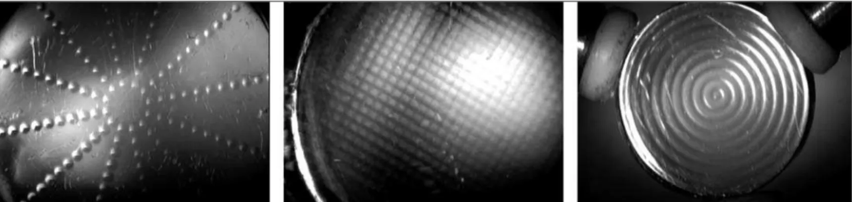
All sensors were manufactured at Eyetec Equipamentos Oftálmicos (www.eyetec.com.br) and at the optical shop of the Physics Department of the University of São Paulo – São Carlos. A computerized lathing machine was used to manufac-ture the molds of the HS and DOD sensors. A high-precision computerized optical carving machine was used to manufactu-re the CYL sensor. Figumanufactu-re 2 shows magnified images of all sensors taken on a Zeiss slit-lamp with 32x and 16x magnifi-cations.
Optical setup
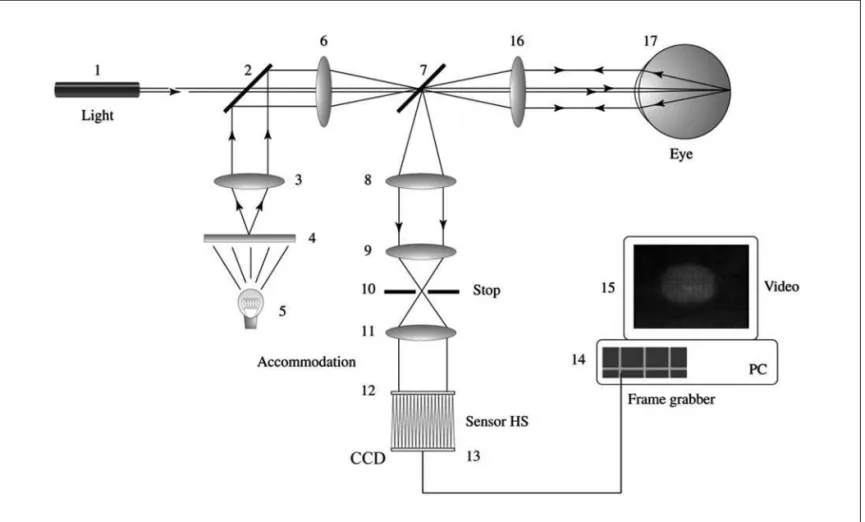
In order to measure the optical aberrations of the mecha-nical eye the optical diagram shown in figure 3 was used.
Figure 1 - (left) Traditional Cartesian-symmetry HS sensor with 25x25 microlenses; (center) HS type sensor but with radial symmetry – which we will call from now on the dodecagonal (DOD) sensor since it has 12 different radial patterns resembling a 12-sided polygon. Liang showed on page 36 of his Master of Science degree thesis(9) a similar sensor but with 8 sides instead of 12. (right) Concentric donut shaped (or Placido shaped) cylindrical sensor proposed here for testing and comparison purposes. Each disc has the effect of a lens and the resulting image
resembles those of the Placido Disc used in videokeratography. We will call it from now on the CYL sensor
Figure 2 - Magnified digital photographs acquired on a Zeiss slit-lamp of the DOD sensor (left), the HS sensor (center), and the CYL sensor (right). The slit-lamp light was positioned transversally such that the microdepressions could be emphasized by their own shadows
sensor (and the other sensors that are subsequently replaced) (12) and is focused at the CCD array (13). The CCD image is digitized in a “frame grabber” (14) and processed by an IBM compatible PC, which displays the graphical information on the colored monitor (15). The actual instrumentation based on
this diagram was mounted on an optical bench and is shown in figure 3 (left).
242 Quantitative comparison of different-shaped wavefront sensors and preliminary results for defocus aberrations on a mechanical eye
manufacture: Eurosys SA., Parc Scientifique du Sart-Tilman, Avenue du Pré-Aily, 14, Angleur, Belgium; home page: www. euresys.com), installed on an IBM compatible PC (Pentium III, 1.1 MHz processor). Once the mechanical eye pupil is in pro-per position, an external pedal is used to trigger image digita-lization.
Image processing
The image processing programs for the HS and CYL sensors were developed in Pascal using the Delphi (www.borland.com) programming language and algorithms from a previous work(10-13).
For the DOD sensor the programming language Matlab (www. mathworks.com), and new algorithms, not yet published, were
Figure 3 - Schematic diagram of optical setup used in our laboratory to measure aberrations of the eye
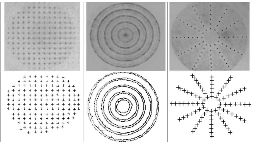
applied. In figure 5 we may see results of the image acquisition and image-processing for each of the wavefront sensors taken for the mechanical eye at emmetropic state.
Zernike polynomials and wavefront fitting
In this section, we’ll briefly demonstrate how the wavefront slopes were fitted for the HS sensor. A complete description is not given here because this topic has been overwhelmingly covered in the literature(8-11,14-16). For the other sensors,
compu-tation is analogous but slope is calculated as partial derivatives relative to radial distance (∂Z/∂ρ) and polar angle (∂Z/∂θ).
The local slope of the wave front for the cylindrical and HS sensors, in the vertical and horizontal directions of the CCD image plane, may be written as
(1a)
(1b)
where and denote the partial derivatives of the wave
aberration function; is the position of the nth spot for the
calibration emmetropic eye (or calibration eye) and is the nth
position for the measured ametropic eye. Our goal is to find the aberration function (W). There are several techniques to find a function from a set of partial derivatives, but the most
popular method in many fields of optics, and also in visual optics, has become the approximation using Zernike polyno-mials(14) and the Least Squares method. We will not get into the
mathematical aspects of why this technique became popular for describing wave aberrations; this is done elsewhere(14-15). What
we may briefly state here is that one of the strongest reasons is that Zernike polynomials form an orthonormal basis and that it has ideal symmetries for describing optical aberrations.
We may write the wave aberration function as
(2)
where C are the coefficients of each polynomial and Z is each term of the Zernike polynomial. The objective is to find these coefficients based on the slopes, so we apply the partial derivatives to equation (2):
(3a)
(3b)
We now use the Least Square method to find the best Zernike coefficients that interpolate the derivatives in (1) and to do that we substitute the values in (3) by the derivatives in (1). We may then write the coefficients as:
C = [MT].[DER] (4)
244 Quantitative comparison of different-shaped wavefront sensors and preliminary results for defocus aberrations on a mechanical eye
Where the coefficient matrix is of the form:
Ci = [C0C1C2...C14]T (5)
(DER) is the column matrix of derivatives, and (MT) is the transformation matrix obtained by the Least Square method. For the CYL and DOD sensors, the calculations are analo-gous. The difference is that the Least Squares fit for the CYL sensor is implemented only for the slope in the radial direction (dZ/dρ) since there is no information regarding polar angle shifts. From the Zernike coefficients, the low order refraction (the sphere-cylinder equivalent) may be obtained, as we follo-wing describe.
Computing the sphere-cylinder equivalent from Zernike coefficients
In order to compare results from the three different sensors with the results from the autorefractor we computed the sphe-re-cylinder equivalent from the Zernike coefficients. This com-putation may be implemented in the following steps:
1) Correct the Zernike coefficient values for chromatic aberration. The wavefront device used in this experiment uses a SLED source operating at 840 nm, but it should be corrected for a user-specified wavelength, which is set to a default value as 550 nm. This value is based on the cone absorption curves of the human retina’s photoreceptors (commercial autorefrac-tors also correct for this wavelength). We have used this wavelength to correct for chromatic aberration for our instru-mentation. The correction formula is:
(6)
where nλ and n840 and are the index of refraction of water at the specified wavelengths. The following equation is an expres-sion that approximates the refraction index of water at any desired wavelength:
(7)
2) Convert specific Zernike coefficients to power vectors, using equations:
(8)
(9)
(10)
where the vector components [J45, M, J180] represent the Jack-son crossed cylinder with axis at 45/135°, the spherical equi-valent and the crossed cylinder at 90/180°. In order to compute the vector components in diopters (D) the pupil diameter and the Zernike coefficients must be in meters. The coefficients in
(8)-(10) correspond, in the VSIA-OSA(17) conventional
nota-tion, to the , and , respectively.
3) Compute the sphere, cylinder and axis of the sphere-cylinder equivalent using the following equations:
(11)
(12)
(13)
where the axis should be written in minus-cylinder, i. e., a value between 0 and 180°.
RESULTS
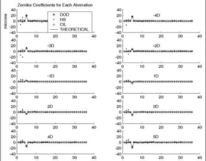
In figure 6 we may see superimposed plots for each sensor for values of all 36 Zernike coefficients for all aberrations, all also the theoretical values.
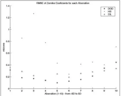
In order to quantify the performance of each sensor for each aberration we computed the root mean square error (RMSE) for all practical Zernike coefficients when compared to the theoretical coefficients. Results are plotted in figure 7.
All graphs above refer to comparisons of our sensors with absolute theoretical values for Zernike coefficients; it is a reasonable analysis in order to quantify absolute precision of each sensor, but it does not take into account probable syste-matic errors of the optical instrumentation. When one is setting up the optical instrumentation depicted in figure 4 there are several practical errors associated with misalignment and improper focusing, which generate systematic errors. In addition, there is no guarantee that the mechanical eye was correctly calibrated (Heine guarantees precisions), etc.
Figure 7 - RMSE of Zernike coefficients for each sensor for all aberra-tions when theoretical data are used as control. The horizontal axis are
labeled from 1 to 10 for aberrations from -5D to +5D
In this sense, another reasonable analysis is to compare results of each sensor for our instrument with that of a second independent instrument. In order to accomplish this we have measured the same aberrations using a commercial autorefrac-tor (Canon model R-50m). Since auautorefrac-torefracautorefrac-tors yield aberra-tions only in the sphere-cylinder format, i. e., the lower order aberrations, we have used equations (6)-(13) to implement a backward computation and extract the 3 sphere-cylinder para-meters from the Zernike coefficients of our previous measure-ments and compared them with those given by the autorefrac-tor. The sphere-cylinder values for each sensor for all aberra-tions may be seen in figure 8.
The RMSE of the three sphere-cylinder parameters for each sensor, taking the theoretical values as control and then the autorefractor as control, may be seen in table 1 and table 2, respectively.
In order to verify if our autorefractor and mechanical eye were calibrated we also computed the RMSE error of each auto-refractor parameter, which is shown in the last row of table 1.
DISCUSSION
As we may see in figure 6, most Zernike coefficients asso-ciated with the low-order sphere-cylinder aberrations (coef-ficients c(4) – c(6)) have similar values for all sensors and all sensors have similar values when compared to the theoretical (continuous curve). In order to quantify how close these coefficients were to the theoretical values we computed the RMSE for all coefficients for each of the aberrations (from -5D to +5D), what is shown in figure 7. Figure 7 tells us that both the CYL and DOD sensors had RMSE of less than 0.4 microns. This is approximately 2% of the peak values (coefficients c(5))
Figure 8 - Sphere, cylinder and axis values for all three sensors (DOD, HS and CYL) and the Canon autorefractor according to computations based on Zernike coefficients shown in figure 6. Theoretical values, based on backward computations using equations (9-13), are also
shown in the continuous curves
Table 1. RMSE for all sphere-cylinder parameters for each sensor when compared to the theoretical data
RMSE (Theoretical values as control)
Sph. Cyl. Axis
DOD 0.1054 0.1531 19.7194
HS 0.2886 0.2777 25.5636
CYL 0.4640 0.1721 18.5631
AUT 0.1140 0.0750 17.0000
Observation: The number of characters after the decimal point has nothing to do with the number of significant characters; we just plotted them in this manner because of the direct output from the Matlab files. Actual practical precision for sphere-cylinder measurements is usually in the second character after the decimal point. Same observation is valid for table 2
Table 2. RMSE for all sphere-cylinder parameters for each sensor when compared to the autorefractor data
RMSE (Autorefractor as control)
Sph. Cyl. Axis
DOD 0.1827 0.1364 34.3596
HS 0.2226 0.2424 35.1636
CYL 0.3517 0.1717 26.3602
246 Quantitative comparison of different-shaped wavefront sensors and preliminary results for defocus aberrations on a mechanical eye
Figures 6 and 7 relate the measured Zernike coefficients for the different aberrations only with theoretical values. Another important analysis that was conducted here is the comparison of values for our sensors with those from a commercial instru-ment. For this purpose, we decided to use a conventional autorefractor. We could have chosen to compare our measure-ments with commercially available wavefront devices (from manufactures such as VISX, Zeiss, etc) but we chose the autorefractor for two reasons: first because it is the most widespread type of automated refraction device available in eye clinics and hospitals throughout the world today; second because there is still an on-going effort by the scientific com-munity in determining the precise relations of optical quality metrics based on wavefront information and their relation to conventional data from visual acuity examinations, such as the autorefractor output and the Snellen optotypes(18-20).
In order to compare our data with those of the autorefrac-tor we had to compute the sphere-cylinder equivalent from our set of 36 Zernike coefficients. The proper way to accomplish this is by applying equations (6)-(13). After computing the sphere-cylinder values, they were plotted in figure 8. The RMSE for sphere, cylinder and axis, for both the theoretical values as control and the autorefractor outputs as control, are shown in tables 1 and 2, respectively.
As we may notice from figure 8 (left), the sphere values for all aberrations for all sensors were very close to the theoretical and to the autorefractor values. A quantitative measure of how close they were to both of these parameters is depicted in column 2 of both tables 1 and 2. The sphere values for the DOD sensor rendered the best results (RMSE of 0.1827D and 0.1054D, respectively). This was quite a surprise since we thought that the conventional HS sensor would surpass the other sensors in all sphere-cylinder parameters, specially the sphere parameter which is more strongly associated with defocus (from equation (12) we may notice that the sphere is the M term minus half the cyl term, and the M term is directly proportional to the c(5) coefficient, therefore the sphere value is more strongly associated with this term). The HS and the CYL sensors also rendered reasonable sphere values (RMSE 0.2886D and 0.4640D for the theoretical values as control, 0.2226D and 0.3517 for autorefractor as control and). Al-though the RMSE for CYL were above conventionally accep-ted values for autorefractors and Snellen chart examinations (between approximately 0.12D and 0.25D) we do not consider this as a limiting factor. The reason for this is that there are many errors associated with an optical bench instrument, such as ours, that are difficult to correct and avoid. These errors include limitations associated with the elimination of spherical aberrations (the lenses used in this experiment had not gone through the process of coating and filtering for optimization regarding the wavelength of the SLED light source), misalignment and improper focus. These are factors optimized in commercial systems because large-scale manu-facturing allows significant reduction in price.
In terms of cylinder, as we may notice from figure 8 (center)
values were also very close to zero for all sensors and also for the autorefractor, as expected. Column 2 of tables 1 and 2 list the values for the RMSE of all these parameters. Both the DOD and CYL cylinder values were below 0.20D for theoretical and autorefractor as control. The HS cylinder values were approxi-mately 0.25D.
The axis values are shown in figure 8 (right). Theoretical and autorefractor values were very close to zero degrees, as expected. Nevertheless, values for the DOD, HS and CYL sensors varied between -50 and 50 degrees, which, at a first glance, seem quite awkward. However, they are not. The explanation for this is that when we are in the process of measuring highly symmetric surfaces, which is the case for the defocus aberration, any deviation in dioptric power along different meridians, no matter how small, will induce values different from zero for Zernike coefficients c(4) and c(6), and therefore astigmatic axis values will be different from zero (see equations (8), (10) and (13)). This aspect has been discussed in a previous work(21) and the assertion is that astigmatic
values for surfaces that are not astigmatic in nature make axis deviations less relevant since the cylinder values are general-ly so small. For this reason we do not consider the deviations shown in figure 8 (right) and column 4 of tables 1 and 2 as drawbacks associated with the principle of wavefront sen-sors, but simply a question of data smoothening in order to eliminate small noises which generate irrelevant astigmatisms. The traditional Hartmann screen has long been applied in many fields of optics. After Shack’s idea in the early 1970’s of using a CCD camera behind the Hartmann screen, it has gene-rally been called the Hartmann-Shack sensor. Since then, it has become quite popular in observatories and other sophisti-cated optical devices such as the Hubble telescope. Neverthe-less, we have shown in this experiment that other sensors of different symmetries and sensors that are based on the Hart-mann principle but with a radial distribution, may also be successfully applied in visual optics.
In this preliminary study, we have taken measurements for only defocus aberrations since we were limited by the availa-ble aberrations on our mechanical eye. Another important analysis for future work is to generate controlled astigmatism of different orders and again compare measurements of wave-front sensors with both the autorefractor outcome and the theoretical values based on backward computations using Zernike coefficients. Moreover, the aberrations collected here (a total of 10 defocus wavefronts) may not be considered statistically significant. There is ongoing work applying the HS sensor to in vivo eyes for statistically significant popula-tions and their relation to conventional acuity measure-ments(18-20). This is perhaps an important step to be taken in
the analysis of different shapes of wavefront sensors. Our general feeling is that, in the same way the Placido Disc has become a gold-standard in videokeratography, even though other patterns were suggested(22-23) and the skewray error was
proven to be relevant in certain cases(24), we also think these
further investigation. For further theoretical considerations regarding more complicated aberration surfaces, such as keratoconus, among others, please refer to a previous work of our group(25).
RESUMO
Objetivo: Sensores de aberrações ópticas de simetria cartesiana
são aceitos pela maioria da comunidade científica como um padrão (como o sensor de Hartmann-Shack (HS)) nos ramos da óptica e da oftalmologia. Neste trabalho foram desenvolvidos e testados três tipos de sensores com simetrias e/ou configura-ções diferentes e foram feitas comparaconfigura-ções entre o sensor de Castro (SC) e o sensor HS na sua forma cilíndrica e cartesiana.
Métodos: Todos os sensores foram projetados e desenvolvidos
em nosso laboratório no Instituto de Física de São Carlos - USP. O primeiro sensor é um sensor HS convencional, ou seja, no formato cartesiano; o segundo é um sensor HS cilíndrico e o terceiro é o SC. Para cada sensor foram realizados tanto cálculos teóricos como medidas práticas em um olho mecânico. O olho mecânico foi ajustado com 10 diferentes tipos de aberrações de desfocalização, de -5D a +5D, em passos de 1D. Resultados: A precisão dos sensores foi analisada utilizando-se dois diferen-tes métodos: primeiramente um método totalmente teórico, ge-rando aberrações com diferentes coeficientes de Zernike e veri-ficando qual a precisão de cada sensor ao calcular estes parâ-metros a partir apenas das derivadas nas direções cartesianas e cilíndricas; segundo, foram realizadas medidas em um olho me-cânico calibrado com estas mesmas aberrações. O resultados para o sensor HS cilíndrico, cartesiano e SC foram, respectiva-mente: erro quadrático médio para valores esfero-cilíndricos quando comparados com o auto-refrator para os três sensores foram 0,18D, 0,22D e 0,35D para esfera, 0,14D, 0,24D e 0,17D para cilindro, 34,36°, 35,16° e 26,36° para eixo; o erro quadrático médio para valores esfero-cilíndricos quando comparados a valores teóricos para os três sensores foram 0,11D, 0,29D e 0,46D para esfera, 0,15D, 0,28D e 0,17D para cilindro, 19,71°, 25,56° e 18,56° para eixo. Conclusão: Nossa conclusão principal é que os três tipos de sensores forneceram resultados seme-lhantes, no entanto há algumas diferenças. Os SC e HS de simetria cilíndrica permitem encontrar o eixo óptico com muito mais facilidade.
Descritores: Técnicas de diagnóstico oftalmológico; Erros de
refração/cirurgia
REFERENCES
1. Thibos LN. Principles of Hartmann-Shack aberrometry. J Refract Surg. 2000; 16(5):S563-5. Review.
2. Scheiner C. Oculus, sive fundamentum opticum. Austria: Innspruk; 1619. 3. Tscherning M. Die monochromatischen Aberrationen des menschlichen Auges.
Z Physiol Psychol Sinne. 1894;6:456-71.
4. Howland B. Use of crossed cylinder lens in photographic lens evaluation. Appl Opt. 1960;7:1587-8.
5. Hartmann J. Bemerkungen über den Bau und die Justierung von Spektrogra-phen. Z Instrumentenkund. 1900;20:47.
6. Shack RV, Platt BC. Production and use of a lenticular Hartmann screen. J Opt Soc Am. 1971;61:656.
7. Paterson C, Dainty JC. Hybrid curvature and gradient wave-front sensor. Opt Lett. 2000;25(23):1687-9.
8. Liang J, Grimm B, Goelz S, Bille JF. Objective measurement of wave aberra-tions of the human eye with the use of a Hartmann-Shack wave-front sensor. J Opt Soc Am A Opt Image Sci Vis. 1994;11(7):1949-57.
9. Liang J. A new method to precisely measure the wave aberrations of the human eye with the Hartamann-Shack-Wavefront-Sensor (thesis). Heidelberg: Universi-ty of Heidelberg; 1991.
10. Carvalho LA. A simple and effective algorithm for detection of arbitrary Hart-mann-Shack patterns. J Biomed Inform. 2004;37(1):1-9.
11. Carvalho LA, Castro JC, Carvalho LA. Measuring higher order optical aberra-tions of the human eye: techniques and applicaaberra-tions. Braz J Med Biol Res. 2002;35(11):1395-406.
12. Carvalho LA, Stefani M, Romao AC, Carvalho L, de Castro JC, Tonissi S, et al. Videokeratoscopes for dioptric power measurement during surgery. J Cataract Refract Surg. 2002;28(11):2006-16.
13. Carvalho L, Tonissi SA, Castro JC. Preliminary tests and construction of a computerized quantitative surgical keratometer. J Cataract Refract Surg. 1999; 25(6):821-6.
14. Born M. Principles of optics: electromagnetic theory of propagation, interferen-ce, and diffraction of light. Oxford; New York: Pergamon Press;1975. p.464-6. 15. Carvalho LA. Preliminary results of neural networks and Zernike polynomials for classification of videokeratography maps. Optom Vis Sci. 2005;82(2):151-8. 16. Guirao A, Artal P. Corneal wave aberration from videokeratography: accuracy and limitations of the procedure. J Opt Soc Am A Opt Image Sci Vis. 2000; 17(6):955-65.
17. Thibos LN, Applegate RA, Schwiegerling JT, Webb R. VSIA Standards Taskforce Members. Vision science and its applications. Standards for reporting the optical aberrations of eyes. J Refract Surg. 2002;18(5):S652-60. 18. Cheng X, Bradley A, Thibos LN. Predicting subjective judgment of best focus
with objective image quality metrics. J Vis. 2004;4(4):310-21.
19. Marsack JD, Thibos LN, Applegate RA. Metrics of optical quality derived from wave aberrations predict visual performance. J Vis. 2004;4(4):322-8. 20. Thibos LN, Hong X, Bradley A, Applegate RA. Accuracy and precision of
objective refraction from wavefront aberrations. J Vis. 2004;4(4):329-51. 21. Carvalho LA. Absolute accuracy of Placido-based videokeratographs to measure
the optical aberrations of the cornea. Optom Vis Sci. 2004;81(8):616-28. 22. Halstead MA, Barsky BA, Klein SA, Mandell RB. A spline surface algorithm
for reconstruction of corneal topography from a videokeratographic reflection pattern. Optom Vis Sci. 1995;72(11):821-7.
23. Halstead MA. Efficient techniques for surface design using constrained optimiza-tion. PhD Dissertaoptimiza-tion. Berkeley: University of California; 1996.
24. Klein SA. Corneal topography reconstruction algorithm that avoids the skew ray ambiguity and the skew ray error. Optom Vis Sci. 1997;74(11):945-62. 25. Carvalho LA, Castro JC. The “Placido” wavefront sensor and preliminary
measurement on a mechanical eye. Optom Vis Sci. In press 2006.