Phytoplankton production modelling in three marine
ecosystems—static versus dynamic approach
M.F. Macedo
a, P. Duarte
b,∗aDepartment Conserva¸c˜ao e Restauro, Faculdade de Ciˆencias e Tecnologia, Universidade Nova de Lisboa, Quinta da Torre,
Monte da Caparica 2829-516 Caparica, Portugal
bCEMAS - Faculdade de Ciˆencia e Tecnologia, Universidade Fernando Pessoa, Pra¸ca 9 de Abril 349, 4200-004 Porto, Portugal
Received 25 February 2004; received in revised form 25 February 2005; accepted 13 May 2005 Available online 21 June 2005
Abstract
Phytoplankton productivity is usually determined from water samples incubated at a number of irradiance levels during several hours. The resultant productivity-irradiance (P–E) curves are then used to estimate local and/or global phytoplankton production. However, there is growing evidence that these curves, referred as static, underestimate phytoplankton photosynthesis to a great deal, by assuming a stable response to light over the incubation period. One of the drawbacks of staticP–Ecurves is the overestimation of photoinhibition.
In this work, three one-dimensional vertically resolved models were developed as simply as possible, to investigate differences between static and dynamic phytoplankton productivity in three marine ecosystems: a turbid estuary, a coastal area and an open ocean ecosystem. The results show that, when photoinhibition development time is considered (dynamic model), the primary production estimates are always higher than when calculated with the static model. The quantitative importance of these differences varies with the type of ecosystem and it appears to be more important in coastal areas and estuaries (from 21 to 72%) than in oceanic waters (10%). Thus, these results suggest that primary production estimates, obtained under the assumption of a static behaviour response to light, may underestimate the real values of global phytoplankton primary production. Calculations suggest that the quantitative importance of this underestimation may be larger than the global missing carbon sink.
© 2005 Elsevier B.V. All rights reserved.
Keywords: Phytoplankton production;P–Erelationship; Static and dynamic modelling; Photoinhibition parameter
∗Corresponding author. Tel.: +351 22 507 13 00;
fax: +351 22 550 82 69.
E-mail addresses:[email protected] (M.F. Macedo), [email protected] (P. Duarte).
1. Introduction
In the last decades, phytoplankton primary pro-duction has received considerable interest due to its relevance as the first link in trophic chains of aquatic ecosystems and the role it plays in the oceanic “biolog-ical pump” for carbon dioxide uptake (Behrenfeld and
Falkowski, 1997). Efforts have been made to describe and understand the carbon fixation at a regional and global scale (Basterretxea and Ar´ıstegui, 2000; Houghton et al., 1990; Longhurst et al., 1995; Mor´an and Estrada, 2001). Nevertheless, there is still a great uncertainty about the magnitude of global primary pro-duction. Estimates vary as much as from 27.1 (Eppley and Peterson, 1979) to 50.2 Gt C y−1(Longhurst et al., 1995). Therefore, the accurate measurement and sim-ulation of theP–Erelationship is of major importance. Generally, the P–E relationship is determined by the incubation of water samples, at several irradiance levels, during a fixed period (2 or 4 h). The resulting
P–Ecurve parameters are then applied to productivity models. These models are referred as static because it is assumed that P–Eparameters are constant over time. The majority of the existing P–E models are static (e.g. Steele, 1962; Vollenweider, 1965; Jassby and Platt, 1976; Fasham and Platt, 1983; Megard et al., 1984).
There are a large number of mathematical formula-tions to describe theP–Erelationship (seeTable 1for a sample of available models and parameters). Some parameters are common to almost all models or can be derived from the models themselves, namely initial slope or photosynthetic efficiency (α), optimal light intensity or the light level that maximizes photosyn-thesis under given nutrient and temperature conditions (Eopt), the light level at which the linear part of the
P–Ecurve intercepts a plateau (light saturation index
-Ek) and the maximal production rate or photosynthetic capacity (Pmax) (Table 1). Parameterαmay be obtained by calculating the limit of the derivative ofPin relation toEasEapproaches zero. In inhibition models,Eopt may be determined by calculating the light intensity that maximizes the same derivative.
Most of the mathematical formulations describing theP–Erelationship are empirical, capable of describ-ing geometrically the observed results, not bedescrib-ing based on physiologic processes (Eqs. (1)–(7) in Table 1). Models such as those presented byFasham and Platt (1983),Eilers and Peeters (1988, 1993)(Eqs. (12) and (13) inTable 1),Megard et al. (1984)(similar to Eilers’ model),Han (2001a,b)andRubio et al. (2003)are of a mechanistic type, derived from known sequences of metabolic transformations. Some assume a saturation curve (Eqs.(1)–(2)and(6)inTable 1), whereas oth-ers consider photoinhibition (i.e. the decline in carbon
fixation at high irradiance) (Eqs. (3)–(5)and(7)–(9) inTable 1). Some are static (Eqs. (1)–(5)and(8) in Table 1) and some are dynamic, considering the effects of time exposure to light on photosynthetic responses, including the development of photoinhibition (e.g. Eqs. (7)and(9)inTable 1).
Experimental evidence suggests that in many cases the static description of the P–E relationship is not appropriate (Marra, 1978; Neale and Marra, 1985; Pahl-Wostl, 1992; Macedo et al., 1998, 2002). In fact, the photosynthetic parameters depend on light intensities recently experienced by the organisms. The irradiance that reaches phytoplankton varies due to diurnal variation in light intensity and vertical mixing process (Denman and Gargett, 1983). Experimental evidence shows that phytoplankton cells may become photoinhibited under high light levels. However, the relative strength of this phenomenon depends on the exposure time to high irradiances (Marra, 1978). There is also some evidence that phytoplankton can maintain high rates of photosynthesis during the first few minutes after initial exposure to saturating or inhibiting irra-diance before photoinhibition takes place (Harris and Lott, 1973; Harris and Piccinin, 1977; Marra, 1978). When irradiance remains very high for a long period, photoinhibition becomes more and more important (Kok, 1956; Takahashi et al., 1971; Harris and Piccinin, 1977; Marra, 1978; Belay, 1981; Whitelam and Codd, 1983; Macedo et al., 1998). On the other hand, pro-duction stops shortly after light is switched off, while recovery from photoinhibition takes longer (Kok, 1956; Belay, 1981). Previous model and experimental results suggest that staticP–Ecurves might lead to a significant underestimation of phytoplankton primary productiv-ity (Duarte and Ferreira, 1997; Macedo et al., 2002).
In spite of the above considerations, most of the
Table 1
Some of the available formulations for theP–Erelationship
Equation Category Type Source
P=Pmax1−exp1−EEk (1) Saturation models Empirical and static Webb et al. (1974)
P=Pmaxtanh
αE
Pmax
,whereα: initial slope (mg C (mg Chla)−1 h−1(µmol quanta m−2s−1)−1
) (2)
Jassby and Platt (1976)
P=Pmax
I Eopt exp
1−EEopt
n
,whereEopt:
optimal light intensity,n=1(nempirical integer) (3)
Photoinhibition models
Steele (1962)
n=1 (4) Parker (1974)
P=Pmax E/Ek
(1+(E/Ek)u)(1+v)/u,different combinations of uandvproduce saturation or inhibition curves (5)
Iwakuma and Yasuno (1983)
P(E, t)=Pt(E, t) tanh
αE
Pt(E,t)
,wherePt(E, t)=
Pmax(E, t) exp
−γ1 t
0E 1/adt
andγ: timescale for photoinhibition (h),a: controls the degree of nonlinearity of the rate response to light intensity (6)
Saturation model Empirical and dynamic Franks and Marra (1994)
P(E, t)= (1−exp(−t/tr)) tanh(E/Ek)
1+(1−exp(−t/ti))Kti(E−Ecrit),whereEcrit: critical light level above which photoihnibition may occur (mmol quanta m−2s−1),t
r:
response time to changing light,ti:
photoinhibition development time (h) (7)
Photoinhibition models
Empirical and dynamic Pahl-Wostl and Imboden (1990)
P= E
aE2+bE+c,see text (8) Mechanistic and static Eilers and Peeters (1988)
P(E, t)= E
(1−exp(−(t/ti)))aE2+bE+c (9) Mechanistic and dynamic Duarte and Ferreira (1997) derived fromEilers and Peeters (1988)and
Pahl-Wostl and Imboden (1990)models (see text)
P– photosynthetic rate (usually expressed as mg C mg Chla−1h−1);P
max– maximum photosynthetic rate;E– light intensity (usually expressed
asmol quanta m−2s−1);Ek– light saturation index;t– exposure time to a particular light level (h) (see text).
Ocean Model (POM) to a lower trophic level food web model, where neither photoinhibition was considered, nor any dynamic link between light history and pho-tosynthetic parameters.Th´ebault and Rabouille (2003) used two mathematical formulations of phytoplankton growth rate as a function of light and temperature. In one of them (Yoyo model), temporal scales of less than a day were considered, accounting for daily sun light variability, using the staticP–Eformulation ofPeeters and Eilers (1978).Robson and Hamilton (2004)applied a three dimensional, coupled hydrodynamic-ecological model to simulate aMicrocystisbloom in an Australian river. Light limitation was based on Steele’s static for-mulation, in the case of freshwater diatoms, and in the saturation type equation described byWebb et al. (1974), in the case of other algae. Finally,Flipo et al. (2004)used the ProSe model, which combines a 1D
hydrodynamic module with a biological one, where the
P–Erelationship is that ofPlatt et al. (1983).
The works cited in the previous paragraph are a clear demonstration of the increasing trend to couple physical and biogeochemical models. Biogeochemical processes are computed at each grid cell, giving place to local changes in pelagic variables, such as phyto-plankton concentration, which are then transported over the model grid by the hydrodynamic model. Using P–E dynamic formulations within the scope of a coupled model implies the resolution of adaptive equations (changing the value of parameters of theP–E
“adaptive status”. This means that after each model iteration, not only the resulting biomass at each model grid cell will depend on local and transport processes, but also the resulting “adaptive status”.
It is conceivable that in a Eulerian vertically resolved mixed layer model, photoinhibited cells at the surface layers may be convected downward, changing the average phytoplankton properties of the destination layers. In such a situation, photoinhibition may develop further downward if the downflux speed is faster than the recovery from photoinhibition, as suggested by the models of Franks and Marra (1994) andDuarte and Ferreira (1997). An opposite situation may result from the upwelling of non-inhibited cells, “diluting” surface inhibited phytoplankton and increasing productivity. Lande and Lewis (1989)compared an Eulerian model similar to the one implemented by the previous authors with a Lagrangian model, that simulated the trajectories of individual cells and respective photoac-climation, retaining information on individual cells, and obtained very similar photosynthetic rates with depth. The small differences observed (<1%) were due to nonlinear dependences of photosynthesis on the
P–Eparameters, in conjunction with the variance and covariance of these traits among cells at given depths. The objective of this work is to evaluate the quan-titative importance of ignoring the dynamic nature of theP–Erelationship in phytoplankton productivity and production estimates in three marine ecosystems, and to assess the impact that this may have on global pro-duction estimates.
2. Materials and methods
In this work, three distinct study areas were selected (an oceanic area, an open coastal area and an estuary) to represent the main types of marine ecosystems, with quite different depths and optical water characteristics. The methodology applied in this work is based on ver-tical productivity profiles calculated, using static and dynamic P–E formulations, for each of the selected ecosystems.
2.1. Study areas
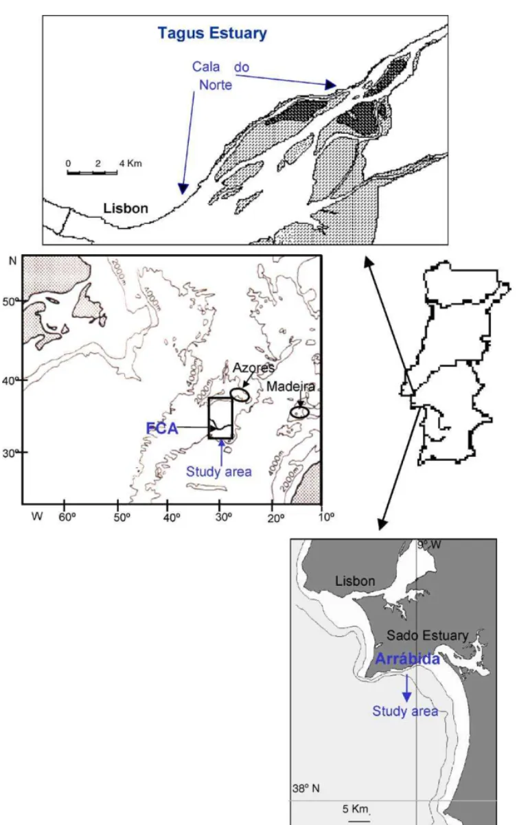
The oceanic area studied was the Azores Front/Cur-rent (FCA), located south of the Azores Archipelago
(Fig. 1). The FCA is a permanent feature throughout the year and it forms part of the sub-tropical North Atlantic gyre (Klein and Siedler, 1989; Alves et al., 1994). Gould (1985) found that the Front could be identified most readily by the position of the 16◦C isotherm at a depth of 200 m. The waters on both sides of the FCA are oligotrophic, with the maximum chlorophyll layer located near the nutricline (Macedo et al., 2001). The open coastal area used in this study is the Arr´abida coast (38◦27′N, 09◦W) located south of
Lisbon (Portugal) (Fig. 1). The sampling location has a depth of 15 m and chlorophyll concentration (Chla) mean values are around 1 mg Chla m−3(Macedo et al., 2002).Fig. 1also shows the Tagus estuary located near Lisbon (38◦50′N, 09◦04′W). Samples were collected in a channel of the Tagus estuary called Cala do Norte. The water is very turbid, with annual values of sus-pended matter ranging from 45 to 120 mg l−1. Salinity ranges from 0 to 32 and is strongly influenced by the semi-diurnal and fortnightly tidal cycle (Ferreira and Ramos, 1989).
Table 2presents the main characteristics of these marine ecosystems. The mean light extinction coef-ficient (k) was calculated from Secchi disk readings. Euphotic depth was calculated as the depth where irra-diance is 1% of its surface value (Parsons et al., 1984).
2.2. Sampling and treatment
Water samples for chlorophyll-a (Chla) determina-tion were collected in the above-mendetermina-tioned ecosys-tems. In the Arr´abida coast and the Tagus estuary, water samples were sieved through a 200m mesh prior to filtration. Filtration was done through 0.45m mem-brane filters. Pigments were extracted in 90% acetone and analysed fluorometrically by the method ofYentsch and Menzel (1963)as modified byHolm-Hansen et al. (1965). Calibrations were performed using Sigma Chla standard. Temperature and salinity were determined in situ with a CTD (Chelsea Instruments) in FCA and with a SCT Meter (YSI model 33) at the other locations.
Table 2
Main characteristics of the marine ecosystems considered in this work
Ecosystem Mean depth (m) Euphotic depth (m) Salinity range k(m−1)
Oceanic (FCA) 1000.0 92.1–46.1 35.1–36.3 0.05–0.1
Coastal (Arr´abida coast) 15.0 23.0 34.5–36.0 0.2
Estuarine (Tagus Estuary) 2.3 1.3 0.0–32.0 3.4
kis the mean light extinction coefficient (see text).
measured using a LICOR spherical quantum sensor (LI-193SA). Light attenuation was achieved with grey PVC nets and preservation of the spectral characteris-tics was checked as described inMacedo et al. (1998). AllP–Eexperiments were performed under controlled temperature, similar to that measured in the field. In each of these experiments two incubation periods were considered: a shorter and a longer one, to obtain static and dynamic P–E curves and parameters. Photosyn-thetic and respiration rate were measured by the oxy-gen incubation technique (Vollenweider, 1974) after the concentration procedure described and validated in Macedo et al. (1998). This procedure was carried out to guarantee phytoplankton concentrations in the incu-bation vessels high enough to allow the usage of the oxygen technique after short incubation periods. It con-sisted of using a towing net with three filtering cones with different gauze (200, 41 and 15m) nested inside each other. Photosynthetic parameters were calculated from theP–Ecurves obtained (seeMacedo et al., 2002).
2.3. Model description
For each of the considered ecosystems a vertically resolved, one-dimensional, hydrodynamic-biological coupled model was used. This model is similar to the one described byDuarte and Ferreira (1997)and was implemented using an object-oriented programming (OOP) approach by means of the EcoWin software (Ferreira, 1995). The hydrodynamic sub-model used in this work was described byPrice et al. (1986)and applied by Janowitz and Kamykowski (1991). Solar and long wave radiation, sensible and latent heat trans-fers across the surface and wind speed are used as forcing functions for the model. In the hydrodynamic sub-model, energy exchanges influence water temper-ature and therefore water density, with implications on water column stability. Wind speed exerts drag at the surface thereby increasing mixing. In the biological sub-model, photosynthetically active radiation (PAR)
forces primary productivity. Estimation of irradiance and radiation fluxes between the sea and the atmo-sphere is based on the formulations described inBrock (1981)andPortela and Neves (1994).
TheEilers and Peeters’s equation (1988) was used to simulate primary productivity as a function of irra-diance (Eq.(10)):
Plight=
E
aE2+bE+c (10)
wherePlight is the light limited primary productivity (h−1),Ethe irradiance level (E m−2s−1) anda,band
care the adjustment parameters. By differentiating the Eilers and Peeters (1988)model as a function of irra-diance, initial slope (α), optimal irradiance level (Eopt) and maximum productivity (Pmax) can be expressed as a function ofa,b, andc:
α=1
c (11)
Eopt=
c
a (12)
Pmax= 1
b+2√ac (13)
The model uses the depth-integrated version of Eq. (10), divided by the height of each vertical layer, in order to compute average productivity (Eq.(14)). The analytical solutions described in Eilers and Peeters (1988)were used to solve this equation:
Plight= 1
z
zbottom
ztop
× Etopexp(−kz)
a(Etopexp(−kz))2+bEtopexp(−kz)+c
∂z
(14)
the depth at layer bottom, respectively, andkis the light extinction coefficient within each layer (m−1).
In this work, some changes to Eilers and Peeters (1988) model were introduced to account for the dynamic aspects of the P–E curves. The photoin-hibition parameter a is recalculated as a function of exposure time to critical irradiance (above the optimal irradiance) according to the DYPHORA model described inPahl-Wostl and Imboden (1990):
a(t)=
1−exp
−tt
i
a (15)
wherea(t) is the parameteraexpressed as a function of time,tthe time exposure to a irradiance aboveEopt andtiis the irradiance inhibition decay time. The value
ofain the second member of Eq.(15)corresponds to fully developed photoinhibition. It was assumed that the recovery from photoinhibition takes the same time as the development of inhibition. This recovery was also calculated from Eq.(15)except that, in this case, it depended on the time under sub-critical irradiance level after the last exposure to critical irradiance. In static simulations the parameterawas constant, whereas in dynamic simulations it was calculated from Eq.(15) as a function of time under photoinhibiting light.
Nitrogen was considered as the limiting nutrient (e.g.Fasham et al., 1990) following studies conducted in the Azores Front (Macedo et al., 2001) and the Tagus estuary (Ferreira and Duarte, 1994). Its effect on phytoplankton growth rate was included by means of a Michaelis–Menten formulation. The ammonium-limiting factor (QNH4) was calculated as follows: QNH4 =
NH4
KNH4+NH4
(16)
where NH4 is the ammonium concentration (mmol m−3) measured in the water and KNH4 is
the half-saturation constant for ammonium uptake. The nitrate-limiting factor was then calculated as follows:
QNO3 =
NO3e−ψNH4
KNO3+NO3
(17)
where NO3 is the nitrate concentration (mmol m−3) measured in the water,KNO3 the half-saturation
con-stant for nitrate uptake andψis a constant equal to 1.5 that parameterises the strength of ammonium inhibition of nitrate uptake (Fasham et al., 1990).
In all simulations, a value of 2 mmol m−3 was assumed for the half-saturation constant for nitrogen limitation (Caplancq, 1990; Lalli and Parsons, 1993).
Finally, the nitrogen and light limited productivity (PN) is given by
PN=Plight(QNH4 +QNO3) (18)
Respiration (R) was computed as a fixed fraction of primary productivity during the day (30%) and as a fixed rate of phytoplankton biomass (10%) during the night. Exudation was calculated as a constant fraction (5%) of primary productivity. The C:Chla ratio was considered constant and equal to 35 mg C mg Chla−1. All these values are within the ranges referred in the literature (e.g. Parsons et al., 1984; Baretta and Ruardij, 1988; Jørgensen et al., 1991). Phytoplankton biomass (B) changes over time were computed by the sum of all gain and loss processes referred above, and from vertical transport computed using the physical sub-model.
All model simulations were performed using static and dynamicP–Eformulations with and without nutri-ent limitation, for a period of 3 days. Simulations were also carried out without wind and with a moderate wind velocity of 10 m s−1. The average gross primary pro-ductivity (GPP) was calculated for each simulation. The time step used in models was calculated, for each ecosystem, as described inPowell et al. (1984).
2.3.1. Oceanic model
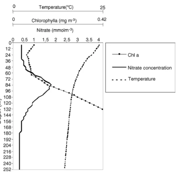
For the FCA model, 63 vertical layers were consid-ered, each with 4 m depth, to simulate a 252 m water column. Mean vertical profiles of nitrate concentration, phytoplankton biomass and water temperature, calcu-lated from in situ measurements (Macedo et al., 2001) were used to set the initial conditions for simulations (Fig. 2).
P–E parameters used in the FCA model were selected within the range of those measured byPlatt et al. (1983)for the Mid-Atlantic Ridge, west of the Azores. According toPahl-Wostl and Imboden (1990), the irradiance inhibition decay time (ti) ranges from 0.5
Fig. 2. Vertical profiles of the Oceanic model initial values: temperature (broken line), nitrate concentration (solid line with circles) and Chla concentration (solid line).
order to reproduce the light irradiance observed during sampling.
2.3.2. Arr´abida model
Thirty vertical layers were considered, each with 0.5 m depth, to simulate a 15 m water column. The values used to initialise the model regarding phyto-plankton biomass, salinity, temperature and nutrient concentrations are presented inTable 4and were deter-mined byMacedo et al. (2002).
For this ecosystem, three sets of simulations were done. Each was based on results from three different
Table 3
Parameters used in the FCA model simulations (see text)
Parameter name Value
k(light extinction coefficient) (m−1) 0.1
ti(light inhibition decay time) (h−1) 1
Pmax(maximum production rate) (h−1) 0.016
α(initial slope) (mg C mg Chla−1h−1
E−1m2s) 0.10
Iopt(optimal irradiance) (E m−2s−1) 87.4
Latitude (◦) 34.5
Simulation days 202–205
P–Eexperiments, hereafter referred as Coastals I, II and III – made in summer, autumn and spring, respectively. The parameters of the P–E curves were determined experimentally using incubation periods from 30 to 180 min (Macedo et al., 2002).P–Eequation parame-ters are presented inTable 5. The model time step used was 0.02 h and all the simulations were performed over a period of 3 days.
2.3.3. Estuarine model
The estuarine model is similar to those mentioned above. Twenty-three vertical layers were considered,
Table 4
Summary of the initial conditions used in the Arr´abida model (see text)
Experiments
I II III
Chla (mg m−3) 0.98 0.39 1.33
Temperature (◦C) 18.5 19.0 14.0
Salinity 34.5 35.5 36.1
Nitrite + nitrate (mmol m−3) 1.8 1.7 2.0
Table 5
Parameters used in the Arr´abida coast model simulations (see text)
Parameter name Value
k(light extinction coefficient) (m−1) 0.2
ti(irradiance inhibition decay time) (h) 3.45 for I 2.5 for II 0.55 for III
Pmax(maximum productivity) (h−1) 0.439 for I
0.301 for II 0.781 for III α(initial slope) (mg C mg Chla−1h−1
E−1m2s)
0.14 for I 0.11 for II 0.26 for III
Iopt(optimal irradiance) (E m−2s−1) 219 for I
220 for II 425 for III
Latitude (◦) 38
Simulation days 255–258 for I
285–288 for II 110–113 for III
each with 0.1 m depth, to simulate a 2.3 m water col-umn. The phytoplankton biomass, salinity and temper-ature measured in situ were used to initialise the model (Table 6). For nitrogen concentration, two different layers were considered: one between the surface and 1.1 m depth and another below 1.1 m. TheP–Ecurve parameters were determined experimentally using two incubation periods: 30 and 120 min (Macedo et al., 2002).Table 7shows the parameters used in this model. The model time step was 2×10⁻⁴h. All the simula-tions were performed over a period of 3 days.
3. Results
3.1. FCA model
The average vertical profiles of water temperature calculated using the model, with and without vertical
Table 6
Initial conditions used in the estuarine model (see text)
Variable Value
Chla concentration (mg m−3) 10.91
Temperature (◦C) 17.0
Salinity 25.0
Nitrate concentration (mmol m−3) 4.31 (surface layer)
2.90 (bottom layer) Ammonia concentration (mmol m−3) 13.45 (surface layer)
12.30 (bottom layer)
Table 7
Parameters used in estuarine model simulations (see text)
Parameter name Value
k(light extinction coefficient) (m−1) 3.4
ti(light inhibition decay time) (h) 1
Pmax(maximum production rate) (h−1) 0.351
α(initial slope) (mg C mg Chla−1h−1
E−1m2s) 0.114 Iopt(optimal irradiance) (E m−2s−1) 353.1
Latitude (◦) 38.5
Simulation days 105–108
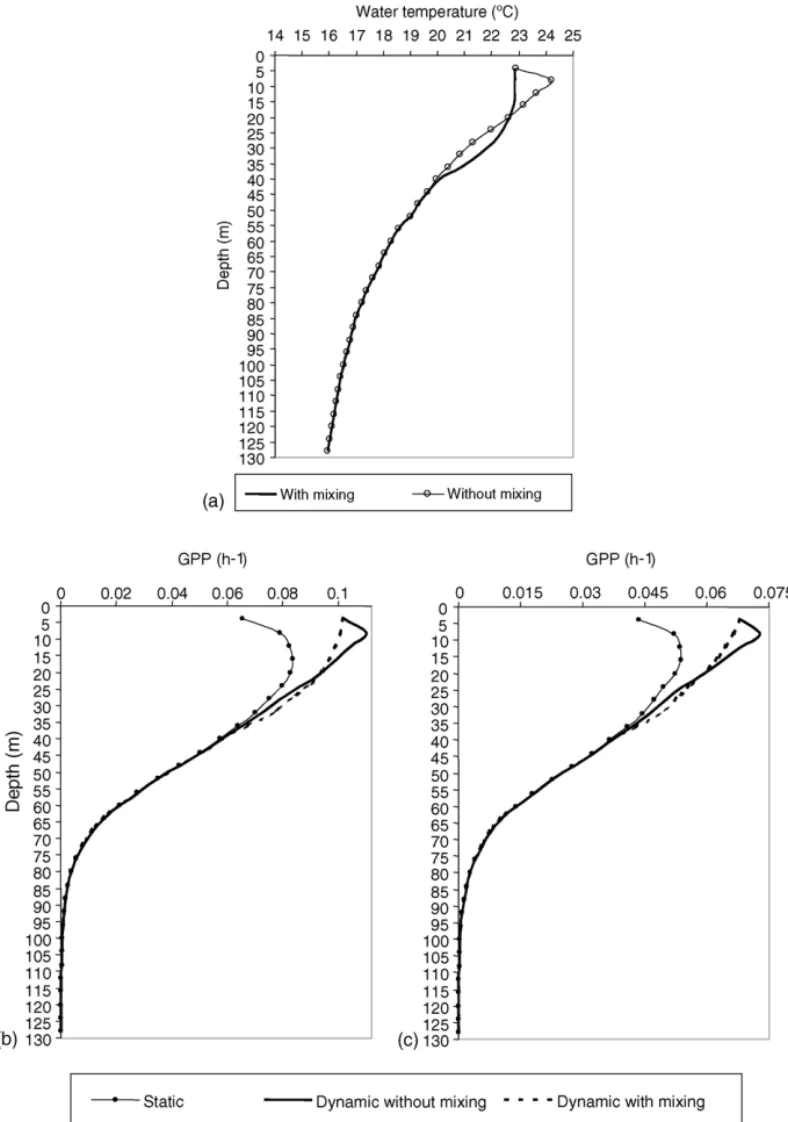
mixing, are presented in Fig. 3a. This figure shows results for the top 130 m being both profiles similar below 45 m depth. Surface temperature values are equal in both simulations (22.9◦C) as expected, since water and air temperature are at equilibrium in this layer. Between 5 and 45 m, the temperature profiles are very different: when vertical mixing is not considered a sub-surface temperature maximum (24.2◦C) occurs at about 8 m whereas, when water mixing is simulated a thermostat (close to 23◦C) appears from the sub-surface down to 20 m depth. Below this depth, between 25 and 45 m, a marked thermocline with about 3◦C of variation is observed. This vertical mixing water tem-perature profile is very similar to the one observed in the field (seeFig. 2). When mixing is not considered, a thermocline with about 4.5◦C of variation is observed between 8 and 45 m.
Average GPP calculated from the Oceanic model with and without nitrogen limitation, is also presented inFig. 3b and c. Dynamic simulations were carried out with and without vertical mixing. Since the GPP is close to zero below 100 m depth, the figure only shows the GPP vertical profile of the upper 130 m. Dynamic simulations present higher GPP values than the static simulations but only in the surface layers, down to 40 m depth. At greater depths, the differences between dynamic and static simulations do not exist. The GPP vertical profiles obtained by the static and dynamic simulations in the surface layers (above 40 m) are very different. The maximum productivity when using static simulations occurs deeper (at about 20 m depth) than in dynamic simulations (at about 5 and 10 m).
Table 8
Water column GPP (mg C m−2h−1) calculated from FCA model
simulations
Model Static Dynamic
without mixing
Dynamic with mixing Without nutrient
limitation
6.83 7.59 7.58
With nutrient limitation
4.44 4.92 4.92
phytoplankton cells do not stay at surface layers long enough for photoinhibition to develop.
Water column integrated GPP values presented in Table 8are similar to those reported byMacedo et al. (2001)for the 15 MW of the FCA. A reduction of water column GPP due to nitrogen limitation is observed both in static and dynamic simulations (Table 8). Nev-ertheless, the vertical profiles of static and dynamic simulations are similar with and without nitrogen lim-itation (Fig. 4b and c). Although water column GPP obtained using the dynamic model was higher than that
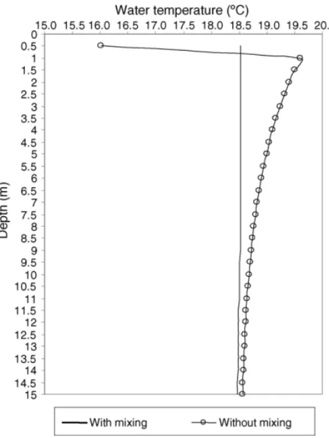
Fig. 4. Average vertical profiles of water temperature, with and with-out vertical mixing, calculated from the Arr´abida coast model.
obtained with the static model, these differences are small (about 10%). The GPP reduction due to nutrient limitation (about 35%) is greater than the differences observed between static and dynamic simulations.
3.2. Arr´abida coast model
Vertical profiles of water temperature calculated with the model, with and without vertical mixing, are presented inFig. 4. A well-mixed water column is obtained when vertical mixture is imposed. The temperature ranges from 18.6◦C, at the surface layer,
to 18.5◦C, at the bottom layer. In this shallow coastal area, the depth of the mixed layer is the same as the total depth (15 m). When no vertical mixing is simulated, the water column becomes stratified with a thin and cold water mass at the surface due to the cooling effect of air temperature. The layer below is the warmer one. These temperature profiles are similar to the ones obtained for the FCA model in the upper layers, down to 20 m depth (Fig. 3a).
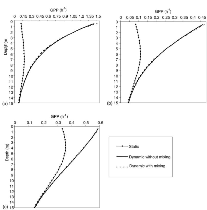
Fig. 5shows average GPP as a function of depth obtained from the three simulation sets of the Arr´abida model. GPP is greater than zero throughout the whole water column. These results are in accordance with the fact that all the water columns is euphotic (seeTable 2). All dynamic simulations showed higher GPP values than the static ones. Furthermore, the vertical GPP profiles from static and dynamic simulations are com-pletely different. The maximum GPP layer observed using the static simulations occurs at around a 7 m depth in Coastal I, 6 m in II and 3.5 m in III; whereas the dynamic simulations presented maximum GPP near surface (Fig. 5). All static simulations exhibited photoinhibition at surface layers but this is not appar-ent in the dynamic simulations. Dynamic simulations with and without mixing were very similar. However, vertical mixing induced a small increase in GPP at the surface layers of the water column (until 1.5 m).
Water column GPP values, with and without nitro-gen limitation, are presented inTables 9 and 10. The reduction in GPP from the dynamic to the static sim-ulation is quite large and it ranges from 21 to 71%, depending on the experiment (Coastal I, II or III). The smaller difference is found in Coastal III and it is due to the smalltivalue (0.55 h). The GPP reduction of water
Fig. 5. Average GPP given by the Arr´abida coast model, with and without vertical mixing, usingP–Eparameters from three different experiments: (a) I; (b) II; (c) III. These simulations were performed without nitrogen limitation (see text).
3.3. Estuarine model
Average vertical profiles of water temperature, with and without vertical mixing, are presented inFig. 6a. These water temperature profiles are very similar to
Table 9
Water column GPP (mg C m−2h−1) calculated from Arr´abida coast
model simulations without nitrogen limitation Static Dynamic
without mixing
Dynamic with mixing
Coastal I 75.14 270.90 271.05
Coastal II 18.52 41.89 41.91
Coastal III 204.10 259.67 259.66
the ones obtained with the Arr´abida coast model simu-lations. A well-mixed water column is obtained when vertical mixture is simulated. Temperature ranged from 19.0◦C, at the surface layer, to 18.75◦C, at the
bot-tom layer. This is a shallow ecosystem (2.3 m) and the
Table 10
Water column GPP (mg C m−2h−1) calculated from the Arr´abida
coast model simulations with nitrogen limitation Model Static Dynamic
without mixing
Dynamic with mixing
Coastal I 39.40 142.0 142.1
Coastal II 9.52 21.5 21.5
Fig. 6. Average vertical profiles of water temperature (◦C) obtained from the estuarine model simulations (a) and average gross primary
Table 11
Water column GPP (mg C m−2h−1) calculated from the estuarine
model simulations with and without nitrogen limitation Model Static Dynamic
without mixing
Dynamic with mixing Without nutrient
limitation
50.95 70.39 70.42
With nutrient limitation
44.3 61.25 61.26
depth of the mixed layer is the same as the total depth. When no vertical mixing is simulated, the water col-umn becomes stratified.
GPP results obtained using the estuarine model are presented in Fig. 6b and c. The dynamic simulation presented higher GPP values than the static simulation. The vertical GPP profiles from static and dynamic sim-ulations are completely different above 0.8 m depth. In static simulations, a surface photoinhibition is observed and a maximum GPP layer is found at 0.3 m, whereas in the dynamic simulations a maximum GPP occurs near the surface (Fig. 6b and c). Below 0.8 m the dif-ferences between static and dynamic simulations dis-appear since the initial slope of theP–Ecurves is the same. In this estuarine area, the water column is very turbid and the photic depth reaches only 1.35 m depth. Bellow 1.70 m GPP is close to zero.
Table 11 presents water column GPP. Dynamic simulation with vertical mixing resulted in slightly higher GPP values than without vertical mixing. This small increase is due to the higher GPP at the surface layers of the water column. The static simulation GPP values are 27% lower. Nitrogen limitation reduced GPP both in the dynamic and in the static simulations (Table 11). However, the difference in GPP observed between static and dynamic simulations is greater than the difference due to nitrogen limitation (about 13%).
4. Discussion
In the FCA model, vertical mixing did not induce significant changes in water column GPP. The reduc-tion in near surface GPP observed in the simulareduc-tions without vertical mixing is due to photoinhibition (Neale, 1987; Long et al., 1994). This resulted from the combination of a lowEopt(87.4E m−2s−1) with
a high water transparency and a low light extinction coefficient (0.1 m−1).
Photoinhibition observed in the static simulation was larger than in the dynamic simulation. This was expected, since photoinhibition is calculated as a func-tion of the exposure time spent above Eopt in the dynamic simulation (see Eq. (15)), whereas in static simulation photoinhibition develops instantaneously. Vertical mixing in the dynamic simulation reduces pho-toinhibition near the surface by reducing the time expo-sure of phytoplankton to high irradiance levels (Duarte and Ferreira, 1997). At the same time, vertical mixing also transports photoinhibited cells to deeper layers, changing population parameters and therefore reducing productivity in those layers. Moreover,Pmaxincreases with a decrease ina(photoinhibition parameter) as can be seen from Eq.(13), therefore, when phytoplankton is exposed to a critical irradiance for a short period of time, GPP may be higher than expected when measured for the same irradiance after a long incubation period. The small differences in the water column predicted GPP, between static and dynamic simulations in the FCA model (about 10%), are explained by the fact that primary production occurs until around 100 m depth but the differences between the vertical GPP profiles are only observed in the first 40 m. At greater depths, there is no distinction in GPP between dynamic and static simulations since the initial slope of the P–E
curves is independent of the photoinhibition parameter (see Eq.(11)).
(Harris and Piccinin, 1977; Marra, 1978; Neale, 1987; Long et al., 1994; Duarte and Ferreira, 1997; Macedo et al., 1998).
Nitrogen limitation influenced both static and dynamic simulations in the same way by reducing GPP without changing its vertical pattern. It is also important to notice that there were three cases (estuarine model and Coastals I and II of Arr´abida model) in which the differences in phytoplankton production between static and dynamic simulations were larger than the differ-ences imposed by nutrient limitation.
For all three ecosystems considered, GPP results from static simulations were always lower than those obtained using dynamic simulations. The magnitude of this difference ranges from 10 to 72% and it appears to be dependent not only on the ecosystem characteristics (e.g. depth, light extinction coefficient, etc.) but also on theP–Ecurve parameters, especially thetiparameter.
The importance of this parameter can be clearly seen in the Arr´abida coast model results (Fig. 5andTable 9). In this model, a lowertivalue (Coastal III), leads to a
smaller difference between static and dynamic simula-tions. When the exposure time to an irradiance above
Eopt is larger than the photoinhibition development time (ti), the a(t) parameter converges to a, which
corresponds to full development of photoinhibition. Nevertheless, it is important to note that in natural conditions, there are many other mechanisms that may influence vertical GPP. For instance, the C:Chla rate is assumed constant in this work, but it may change with temperature, light intensity and nutrient concentration (Cloern et al., 1995). In the estuarine model, vertical mixing is simulated as being only dependent on the wind, but in natural conditions it is mostly influenced by tidal currents and river flows. These will probably have a much stronger effect in reducing the exposure time of phytoplankton cells to inhibiting light intensity. These aspects were not considered in this paper since the aim of the present work was to keep the models as simple as possible in order to highlight the differences between static and dynamic simulations.
The results presented in this work suggest the impor-tance of considering the variability ofP–Eparameters in photosynthesis modelling. This implies increasing he physiological detail of models. Some authors argue that more physiological detail does not necessarily improve the performance of ecosystem models (e.g. Fulton et al., 2004), in clear opposition to our results.
There is an emergent modelling approach using dynamic formulations for model parameters – Structurally Dynamic Modelling (Jørgensen and Bendoriccchio, 2001). According to these authors, in these models, parameters are changed according to some goal function, such as the maximum power prin-ciple, ascendancy or exergy. Therefore, the use ofP–E
dynamic formulations is well within the spirit of recent developments in ecological modelling, with the dif-ference that parameters are calculated in a determinist way, whereas in models using goal seeking functions, typically (e.g.Zhang et al., 2003, 2004), new parameter combinations are chosen by trial and error, to maximize the goal seeking function. The two approaches are not incompatible and may be used in the same model for different parameters, according to available knowledge on their mutual covariance and/or quantitative relation-ships and between them and environmental conditions.
5. Conclusions
In this work, three one-dimensional vertical models were elaborated as simply as possible, to investigate the differences between predicted GPP using a static and a dynamicP–Eformulation. Dynamic simulations showed GPP values higher than those predicted using static models.
al. (1995). Moreover, this range of values is higher than the missing carbon sink of 1.6 Gt C y−1 (Sundquist, 1993; Mann and Lazier, 1996). Although these calcu-lations are merely speculative, they help us understand the potential importance of considering the dynamic behaviour of the photoinhibition parameters in GPP estimates, when theP–Erelationship is used in math-ematical models. The drawbacks of using dynamic
P–E models are their larger number of parameters, requiring more detailed photosynthetic studies, and the larger computation time, that should be considerable smaller than the time scales of dynamic processes.
Acknowledgements
This work was supported by Fundac¸˜ao para a Ciˆencia e Tecnologia PhD grant BD/4146/96.
References
Alves, M.A., Sim˜oes, A, Verdi´ere, A.C., Juliano, M., 1994. Atlas Hydrologique Optimale pour l’Atlantique Nord-Est et Centrale Nord (0–50◦W, 20–50◦N). Universit´e des Ac¸ores, 76 pp. Baretta, J., Ruardij, P., 1988. Tidal flat estuaries. Simulation and
Analysis of the Ems Estuary. Springer-Verlag, Berlin. Basterretxea, G., Ar´ıstegui, J., 2000. Mesoscale variability in
phy-toplankton biomass distribution and photosynthetic parameters in the Canary-NW African coastal transition zone. Marine Ecol. Progr. Ser. 197, 27–40.
Behrenfeld, M.J., Falkowski, P.G., 1997. Photosynthetic rates derived from satellite-based chlorophyll concentration. Limnol. Oceanogr. 42, 1–20.
Belay, A., 1981. An experimental investigation of inhibition of phy-toplankton photosynthesis at lake surfaces. New Phytologist 89, 61–74.
Berger, W.H., Fisher, K., Lai, C., Wu, G., 1987. Oceanic primary productivity and organic carbon flux. Part 1. Overview and maps of primary production and export. Scripps Inst. Oceanogr. 87-30, 1–67.
Bonnet, M.P., Wessen, K., 2001. ELMO, a 3D water quality model for nutrients and chlorophyll: first application on a lacustrine ecosystem. Ecol. Model. 141, 19–33.
Brock, T.D., 1981. Calculating solar radiation for ecological studies. Ecol. Model. 14, 1–19.
Caplancq, J., 1990. Nutrient dynamics and pelagic food web interac-tions in oligotrophic and eutrophic environments: an overview. Hydrobiologia 207, 1–14.
Cloern, J.E., Grenz, C., Videgar-Lucas, L., 1995. An empirical model of the phytoplankton chlorophyll:carbon ratio - the conversion factor between productivity and growth rate. Limnol. Oceanogr. 40, 1313–1321.
Chen, C., Ji, R., Schwab, D.J., Beletsky, D., Fahnenstiel, G.L., Jiang, M., Johengen, T.H., Vanderploeg, H., Eadie, B., Budd, J.W., Bundy, M.H., Gardner, W., Cotner, J., Lavrentyev, P.J., 2002. A model study of the coupled biological and physical dynamics in Lake Michigan. Ecol. Model. 151, 154–168.
Denman, K.L., Gargett, A.E., 1983. Time and space scales of vertical mixing and advection of phytoplankton in upper ocean. Limnol. Oceanogr. 28, 801–815.
Duarte, P., Ferreira, J.G., 1997. Dynamic modelling of photosynthe-sis in marine and estuarine ecosystems. Environ. Model. Assess. 2, 83–93.
Eilers, P.H.C., Peeters, J.C.H., 1988. A model for the relationship between light intensity and the rate of photosynthesis in phyto-plankton. Ecol. Model. 42, 199–215.
Eilers, P.H.C., Peeters, J.C.H., 1993. Dynamic behaviour of a model for photosynthesis and photoinhibition. Ecol. Model. 69, 113–133.
Eppley, R.W., Peterson, B.W., 1979. Particulate organic matter flux and phytoplanktonic new production in deep ocean. Nature 285, 677–680.
Fasham, M.J.R., Platt, T., 1983. Photosynthetic response of phyto-plankton to light: a physiological model. Proc. R. Soc. London B 219, 355–370.
Fasham, M.J.R., Ducklow, H.W., McKelvie, S.M., 1990. A nitrogen-based model of plankton dynamics in the oceanic mixed layer. J. Marine Res. 48, 591–639.
Ferreira, J.G., 1995. ECOWIN – An object-oriented ecological model for aquatic ecosystems. Ecol. Model. 79, 21–34.
Ferreira, J.G., Ramos, L., 1989. A model for the estimation of annual production rates of macrophyte algae. Aquat. Bot. 33, 53–70. Ferreira, J.G., Duarte, P., 1994. Productivity of the Tagus estuary: an
application of the EcoWin ecological model. Gaia 8, 89–95. Flipo, N., Even, S., Poulin, M., Tusseau-Vuillemin, M.-H.,
Ameziane, T., Dauta, A., 2004. Biogeochemical modelling at the river scale: plankton and periphyton dynamics Grand Morin case study, France. Ecol. Model. 176, 333–347.
Franks, P.J.S., Marra, J., 1994. A simple new formulation for phy-toplankton photoresponse and an application in a wind-driven mixed-layer model. Marine Ecol. Progr. Ser. 111, 143–153. Fulton, E.A., Parslow, J.S., Smith, A.D.M., Johnson, C.R., 2004.
Biogeochemical marine ecosystem models II: the effect of phys-iological detail on model performance. Ecol. Model. 173, 371– 406.
Goldman, J.C., Dennett, M.R., 1984. Effect of photoinhibition dur-ing bottle incubations on the measurement of seasonal primary production in a shallow coastal water. Marine Ecol. Progr. Ser. 15, 169–180.
Gould, W.J., 1985. Physical oceanography of the Azores Front. Progr. Oceanogr. 14, 167–190.
Han, B.-P., 2001a. Photosynthesis-irradiance response at physiolog-ical level: a mechanistic model. J. Theor. Biol. 213, 121–127. Han, B.-P., 2001b. A mechanistic model of algal photoinhibition
induced by photodamage to phosystem-II. J. Theor. Biol. 214, 519–527.
Harris, G.P., Piccinin, B.B., 1977. Photosynthesis by natural phyto-plankton populations. Arch. Hydrobiol. 59, 405–457.
Holm-Hansen, O., Lorenzen, C.J., Holmes, R.W., Strickland, J.D.H., 1965. Fluorometric determination of chlorophyll. J. Cons. Int. Explor. Mer. 30, 3–15.
Houghton, J.T., Jenkins, G.J., Ephraums, J.J., 1990. Climate Change: The IPCC Assessment. Cambridge University Press, Cambridge, UK.
Iwakuma, T., Yasuno, M., 1983. A comparison of several math-ematical equations describing photosynthesis-light curve for natural phytoplankton populations. Arch. Hydrobiol. 97, 208– 226.
Janowitz, G.S., Kamykowski, D., 1991. An Eulerian model of phy-toplankton photosynthetic response in the upper mixed layer. J. Plankt. Res. 13, 988–1002.
Jassby, A.D., Platt, T., 1976. Mathematical formulation of the rela-tionship between photosynthesis and light for phytoplankton. Limnol. Oceanogr. 21, 540–547.
Jørgensen, S.E., Nielsen, S.N., Jørgensen, L.A., 1991. Handbook of Ecological Parameters and Ecotoxicology. Elsevier, London. Jørgensen, S.E., Bendoriccchio, G., 2001. Fundamentals of
Ecolog-ical Modelling. Elsevier Science.
Klein, B., Siedler, G., 1989. On the origin of the Azores Current. J. Geophys. Res. 94, 6159–6168.
Kok, B., 1956. On the inhibition of photosynthesis by intense light. Biochim. Biophys. Acta 21, 234–244.
Lalli, C.M., Parsons, T.R., 1993. Biological Oceanography: An Intro-duction. Butterworth-Heinemann Ltd, Oxford.
Lande, R., Lewis, M.R., 1989. Models of photoadaptation and pho-tosysnthesis by algal cells in a turbulent mixed layer. Deep-Sea Res. 36, 1161–1175.
Long, S.P., Humphries, S., Falkowski, P.G., 1994. Photoinhibition of photosynthesis in nature. Annu. Rev. Plant Mol. Biol. 45, 655–662.
Longhurst, A., Sathyendranath, S., Platt, T., Caverhill, C., 1995. An estimate of global primary production in the ocean from satellite radiometer data. J. Plankt. Res. 17, 1245–1271.
Macedo, M.F., Ferreira, J.G., Duarte, P., 1998. Dynamic behaviour of photosynthesis-irradiance curves determined from oxygen pro-duction during variable incubation periods. Marine Ecol. Progr. Ser. 165, 31–43.
Macedo, M.F., Duarte, P., Ferreira, J.G., Alves, M., Costa, V., 2001. Analysis of the deep chlorophyll maximum across the Azores front. Hydrobiologia 441, 155–172.
Macedo, M.F., Duarte, P., Ferreira, J.G., 2002. The influence of incubation periods on photosynthesis-irradiance curves. J. Exp. Marine Biol. Ecol. 274, 101–120.
Mann, K.H., Lazier, J.R.N., 1996. Dynamics of Marine Ecosystems. Biological–Physical Interactions in the Oceans, 2nd ed. Black-well Science, Massachusetts, USA.
Marra, J., 1978. Phytoplankton photosynthetic response to vertical movement in mixed layer. Marine Biol. 46, 203–208.
Megard, R.O., Tonkyo, D.W., Senft, W.H., 1984. Kinetics of oxy-genic photosynthesis in planktonic algae. J. Plankt. Res. 6, 325–337.
Mor´an, X.A.G., Estrada, M., 2001. Short-term variability of pho-tosynthetic parameters and particulate and dissolved primary
production in the Alboran Sea (SW Mediterranean). Marine Ecol. Progr. Ser. 212, 53–67.
Neale, P.J., 1987. Algal photoinhibition and photosynthesis in the aquatic environment. In: Kyle, D.J., et al. (Eds.), Photoinhibition. Elsevier.
Neale, P.J., Marra, J., 1985. Short-term variation of Pmax under nat-ural irradiance conditions: a model and its implications. Marine Ecol. Progr. Ser. 26, 113–124.
Omlin, M., Reichert, P., Forster, R., 2001. Biogeochemical model of Lake Z¨urich: model equations and results. Ecol. Model. 141, 77–103.
Oguz, T., Malanotte-Rizzoli, P., Ducklow, H.W., 2001. Simulations of phytoplankton seasonal cycle with the level and multi-layer physical-ecosystem models: the Black Sea example. Ecol. Model. 144, 295–314.
Pahl-Wostl, C., 1992. Dynamic versus static models for photosyn-thesis. Hydrobiologia 238, 189–196.
Pahl-Wostl, C., Imboden, D.M., 1990. DYPHORA – a dynamic model for the rate of photosynthesis of algae. J. Plankt. Res. 12, 1207–1221.
Parker, R.A., 1974. Empirical functions relating metabolic processes in aquatic systems to environmental variables. J. Fish. Res. Board Canada 31, 1150–1552.
Parsons, T.R., Takahashi, M., Hargrave, B., 1984. Biological Oceano-graphic Processes. Pergamon Press, New York.
Peeters, J.C.H., Eilers, P.H.C., 1978. The relationship between light intensity and photosynthesis. A simple mathematical model. Hydrobiol. Bull. 12, 134–136.
Platt, T., Subba Rao, D.V., Irwin, B., 1983. Photosynthesis of picoplankton in the oligotrophic ocean. Nature 301, 702– 704.
Portela, L.I., Neves, R., 1994. Modelling temperature distribution in the shallow Tejo estuary. In: Tsakiris, Santos (Eds.), Advances in Water Resources Technology and Management. Balkema, Rot-terdam, pp. 457–463.
Powell, T.M., Kirkish, M.H., Neale, P.J., Richerson, P.J., 1984. The diurnal cycle of stratification in Lake Titicaca: eddy diffusion. Verh. Int. Verein. Linmol. 22, 1237–1243.
Price, J.F., Weller, R.A., Pinkel, R., 1986. Diurnal cycling: obser-vations and models of the upper ocean response to diurnal heating, cooling, and wind mixing. J. Geophys. Res. 91, 8411– 8427.
Robson, B.J., Hamilton, D.P., 2004. Three-dimensional modelling of aMicrocystisbloom event in the Swan River estuary, Western Australia. Ecol. Model. 174, 203–222.
Rubio, F.C., Camacho, F.G., Sevilla, J.M.F., Chisti, Y., Molina, E., 2003. A mechanistic model of photosynthesis in microalgae. Biotechnol. Bioeng. 81, 459–473.
Steele, J.H., 1962. Environmental control of photosynthesis in the sea. Limnol. Oceanogr. 7, 137–150.
Sundquist, E.T., 1993. The global carbon dioxide budget. Science 259, 934–941.
Takahashi, M., Shimura, S., Yamaguchi, Y., Fujita, Y., 1971. Pho-toinhibition of phytoplankton photosynthesis as a function of the exposure time. J. Oceanogr. Soc. Jpn. 27, 43–50.
as a function of light and temperature, in two simulation models (Aster & Yoyo). Ecol. Model. 163, 145–151.
Vollenweider, R.A., 1965. Calculation models of photosynthesis – depth curves and some implications regarding daily estimates in primary production measurements. Mem. Ist. Ital. Idrobiol. 18, 425–427.
Vollenweider, R.A., 1974. A Manual on Methods for Measuring Pri-mary Productivity in Aquatic Environments. Blackwell, Oxford, 225 pp.
Webb, W.L., Newton, M., Starr, D., 1974. Carbon dioxide exchange of Alnus rubra: a mathematical model. Oecologia 17, 281– 291.
Whitelam, G.C., Codd, G.A., 1983. Photoinhibition of photosynthe-sis in the cyanobacteriumMicrocystis aeroginosa. Planta 157, 561–566.
Yentsch, C.S., Menzel, D.W., 1963. A method for the determination of phytoplankton chlorophyll and phaeophytin by fluorescence. Deep Sea Res. 10, 221–231.
Zhang, J., Jørgensen, S.E., Tan, C.O., Beklioglu, M., 2003. A struc-turally dynamic modelling-Lake Morgan, Turkey as a case study. Ecol. Model. 164, 103–120.