Lat. Am. j. solids struct. vol.13 número13

Abstract

A three-dimensional rail-bridge coupling element of unequal lengths in which the length of the rail element is shorter than that of the bridge element is presented in this paper to investigate the spatial dynamic responses of a train-track-bridge interaction sys-tem. Formulation of stiffness and damping matrices for the fasten-er, ballast, and bearing, as well as the three-dimensional equations of motion in matrix form for a train-track-bridge interaction sys-tem using the proposed element are derived in detail using the energy principle. The accuracy of the proposed three-dimensional rail-bridge coupling element is verified using the existing two-dimensional element. Three examples of a seven-span continuous beam bridge are shown: the first investigates the influence of the efficiency and accuracy of the lengths of the rail and bridge ele-ments on the spatial dynamic responses of the train-track-bridge interaction system, and the other two illustrate the influence of two types of track models and two types of wheel-rail interaction models on the dynamic responses of the system. Results show that (1) the proposed rail-bridge coupling element is not only able to help conserve calculation time, but it also gives satisfactory results when investigating the spatial dynamic responses of a train-track-bridge interaction system; (2) the double-layer track model is more accurate in comparison with the single-layer track model, particularly in relation to vibrations of bridge and rail; and (3) the no-jump wheel-rail interaction model is generally reliable and efficient in predicting the dynamic responses of a train-track-bridge interaction system.

Keywords

Three-dimensional rail-bridge, coupling element, unequal length, bridge, track, finite element method

Three-Dimensional Rail–Bridge Coupling Element of Unequal

Lengths for Analyzing Train–Track–Bridge Interaction System

Zhi-Ping Zeng a Fu-Shan Liu a,* Zhao-Hui Lu a Zhi-Wu Yu a Ping Lou a Ling-Kun Chen b

a _{School of Civil Engineering, Central} South University, Changsha 410075, China.

b _{College of Civil Science and Engineering,} Yangzhou University, Yangzhou 225127, China.

Corresponding author:

* _{fushan0716@qq.com (Fu-Shan Liu)}

http://dx.doi.org/10.1590/1679-78252551

1 INTRODUCTION

A considerable amount of research has been conducted on the dynamic responses of railway bridge/track structures subjected to a moving train (Sun and Dhanasekar, 2002; Liu et al., 2009; Lu et al., 2009; Wang et al., 2010; Kim, 2011; Zakeri et al., 2014; Lei and Wang, 2014; Xu et al., 2015). Such research has been conducted particularly in the past three decades and mostly in relation to the rapid development of high-speed railways worldwide. However, due to the massive volume of work conducted, it is difficult to have a complete count of the number of studies and it is only pos-sible to cite a few of those that are most relevant here.

The dynamic response of structures in relation to moving vehicles has been studied by previous researchers by modeling a moving vehicle as a moving load, moving mass, or a moving sprung mass with consideration of suspension (Ayre et al., 1950; Frýba, 1972; Chu et al., 1979; Wu and Dai, 1987; Chatterjee et al., 1994; Ichikawa et al., 2000). More sophisticated models that also consider the vertical dynamic interaction between the moving train and structures have also been imple-mented by a large number of researchers in recent years. For example, Zhai and Sun (1994) devel-oped a new and detailed model to investigate the vertical interaction between a vehicle and the track in which the vehicle was modeled as a multi-body system with 10 degrees of freedom (DOFs), the track as an infinite Euler beam, and the wheel–rail interaction as a Hertzian nonlinear contact spring. In addition, Yang et al. (1999) derived a vehicle–bridge interaction element by considering a vehicle as a rigid beam supported by two suspension units and a bridge as beam elements, and Cheng et al. (2001) proposed a bridge-track-vehicle element in which the vehicles were modeled as mass-spring-damper systems, the rails as an upper beam element, and the bridge deck as a lower beam element. Furthermore, Lei and Noda (2002) developed a dynamic computational model for a vehicle and track coupling system using the finite element method (FEM), in which the vehicle-track coupling dynamic responses were analyzed in time and frequency domains due to the random irregularity of the track vertical profile. Thereafter, Wu and Yang (2003) investigated the vertical dynamic responses of a vehicle-rails-bridge interaction system using a condensation technique, which included the steady-state response and riding comfort of the train as well as the impact response of the rails and bridges. Based on the principle of a stationary value of total potential energy of dy-namic system, Zeng (2003), Lou (2005), and Lou and Zeng (2005) derived equations of motion in a matrix form for three types of vehicle-track-bridge vertical interaction elements, in which the rails and the bridge deck were represented by an elastic Bernoulli-Euler upper beam with finite length and a simply supported Bernoulli-Euler lower beam, respectively. A later study by Lou (2007) in-vestigated the vertical dynamic responses of a train-track-bridge interaction (TTBI) system using FEM, and by discretizing the slab track subsystem into track elements that flow with the moving vehicle, Lei and Wang (2014) developed a new approach with finite elements in a moving frame of reference to investigate the dynamic behavior of the train and slab track coupling system.

system, and the derailment and the offload factors related to the running safety of the train, using a 3D finite element model to represent the bridge. Furthermore, Wu et al. (2001) developed a vehicle-rail-bridge interaction model to analyze the 3D dynamic interaction between moving trains and the railway bridge, and Dinh et al. (2009) developed a formulation for 3D dynamic interactions between a bridge and a high-speed train using wheel-rail interfaces, where the bridge eccentricities and deck displacement due to torsion were accounted for in bridge deck modeling. Papers have also been written addressing the dynamic interaction between the track/bridge and the moving train, and some monographs have focused on this subject. For example, Song et al. (2003), Kwasniewski et al. (2006), Nguyen et al. (2009), Lei and Zhang (2011), Xin and Gao (2011), and Zhai et al. (2013) proposed a theory and method for dealing with the dynamic problem of the vehicle-track/bridge interaction system, respectively.

In the aforementioned works, most researchers have established the track-bridge interaction model using FEM, in which a rail-bridge coupling element of equal lengths (i.e., with the length of the rail element equal to that of the bridge element) is adopted. When the length of the bridge in-creases, the DOFs of the track-bridge interaction system also increase, and thus making a dynamic analysis of a track-bridge interaction system is a relatively time consuming process when using a rail-bridge coupling element of equal lengths. Therefore, the aim of this paper is to present a 3D rail-bridge coupling element of unequal lengths, in which sleepers are considered and where the length of the bridge element is longer than that of the rail element, to investigate the spatial dy-namic responses of a TTBI system under the action of track irregularities. This paper can therefore be regarded as an extension of the theory presented by Lou et al. (2012), in which a 2D (vertical) rail-bridge coupling element of unequal lengths was proposed to analyze the vertical dynamic re-sponses of a TTBI system. However, the possibility of considering the lateral rere-sponses of a TTBI system in the current work allows for a more realistic analyses.

In this study, a seven-span continuous beam bridge is used as an example, the influences of the lengths of the bridge and rail elements, two types of track models, and two types of wheel-rail in-teraction models on the efficiency and accuracy for calculating the spatial dynamic responses of the TTBI system excited by track irregularities are carried out, based on which some conclusions are drawn.

2 A 3D RAIL-BRIDGE COUPLING ELEMENT OF UNEQUAL LENGTHS

2.1 Model

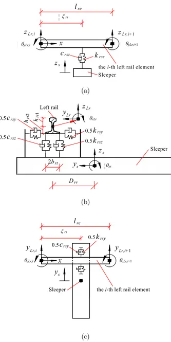
also include a bearing that connects a pier node at a supporting point of the bridge. The rails, bridges, and piers are modeled as uniform Bernoulli-Euler beams, while each sleeper is modeled as a rigid body, and the lateral and vertical elasticity and damping properties of the fastener, ballast, and bearing are modeled using discrete massless springs and dampers. The mass of the ballast is also added to the dead load of the bridge. As the longitudinal vibrations are neglected, each node in the rail and bridge elements has five DOFs, i.e., a lateral displacement along the y-axis, a vertical displacement along the z-axis, and three rotations about the x-, y-, and z-axes. Each sleeper and

each node in the pier element has three DOFs, i.e., a lateral displacement along the y-axis, a

verti-cal displacement along the z-axis, and a rotation about the x-axis. The positive directions of these DOFs accord with those of the co-ordinate, as shown in Figure 1. In addition, it is assumed that the length of the bridge element (LBE) is an integer number of times of the length of the rail element (LRE).

(a)

(b)

(c)

Figure 1: Typical 3D rail–bridge coupling element of unequal lengths: (a) frontal view, (b) left side view, and (c) top view.

lsp

Bridge element

x z

/2 lre lsp

lbe

¦ Èy

pe l

Sleeper Fastener Ballast Rail element

Pier element

Pier

0.5 0.5

bt1

h

k

k 0.5

h

bbz

bby

2D

D ¦ È

c c

cbb ctb

z 0.5

x bt2

bbz bby Bearing y

sbz sby rsz crsy

Right rail

bal Left rail

2D rr

2D

Bridge

k

csbz ksby

c k crsz

krsy

x y

Left rail Sleeper

Bridge ¦ Èz

Right rail Left fastener

Right fastener

θy

θx

Track

Notation Parameter Value Ar (m2) Sectional area of rail 77.45E-4

Er (N/m2) Young’s modulus of rail 2.10E11

Gr (N/m2) Shear modulus of rail 8.08E-10

݉ഥ௥ (kg/m) Mass per unit length of rail 60.64

hrt1 (m) Vertical distance between rail top and its center of torsion 94.53E-3

hrt2 (m) Vertical distance between rail bottom and its center of torsion 81.47E-3

brt (m) Half of width of rail bottom 75.00E-3

lre (m) Length of rail element (LRE) -

Irx (m4) Torsional moment of inertia about x-axis of rail 2.43E-5 Iry (m4) Flexural moment of inertia about y-axis of rail 3.22E-5

Irz (m4) Flexural moment of inertia about z-axis of rail 5.24E-6

ms (kg) Mass of a sleeper 340

Jsx (kg·m2) Moment of inertia about x-axis of sleeper 74.2

lsp (m) Sleeper space 0.625

Drr (m) Half of transverse distance between center lines of two rails 0.75

Dbal (m) Half of transverse distance between the two supporting points of ballast 0.75 krsy (N/m) Lateral stiffness of discrete spring reflecting the property of fastener 3.0E7

krsz (N/m) Vertical stiffness of discrete spring reflecting the property of fastener 6.0E7 crsy (N·s/m) Lateral damping coefficient of discrete damper reflecting the property of fastener 5.0E4 crsz (N·s/m) Vertical damping coefficient of discrete damper reflecting the property of fastener 7.5E4

ksby (N/m) Lateral stiffness of discrete spring reflecting the property of ballast under single rail 5.0E7 ksbz (N/m) Vertical stiffness of discrete spring reflecting the property of ballast under single rail 2.25E8

csby (N·s/m) Lateral damping coefficient of discrete damper reflecting the property of ballast under

single rail 4.0E4

csbz (N·s/m) Vertical damping coefficient of discrete damper reflecting the property of ballast under

single rail 6.0E4

Bridge

Notation Parameter Value Ab (m2) Sectional area of bridge 12.83

Eb (N/m2) Young’s modulus of bridge 3.45E10

Gb (N/m2) Shear modulus of bridge 1.44E10

݉ഥ௕ (kg/m) Mass per unit length of bridge 4.38E10

hbt1 (m) Vertical distance between bridge deck and its center of torsion 1.42

hbt2 (m) Vertical distance between bridge bottom and its center of torsion 1.88

Dctb (m) Half of transverse distance between center lines of two tracks 2.5

Dcbb (m) Half of transverse distance between center lines of bearing 2.4

lbe (m) Length of bridge element (LBE) -

Ibx (m4) Torsional moment of inertia about x-axis of bridge 51.9

Iby (m4) Flexural moment of inertia about y-axis of bridge 19.2 Ibz (m4) Flexural moment of inertia about z-axis of bridge 134.0 kbby (N/m) Half of lateral stiffness of discrete spring reflecting the property of bearing 2.5E8

cbby (N·s/m) Half of lateral damping coefficient of discrete damper reflecting the property of bearing 1.0E5 cbbz (N·s/m) Half of vertical damping coefficient of discrete damper reflecting the property of bearing 1.0E6

ζb Damping ratio of bridge 0.05

Pier

Notation Parameter Value Ap (m2) Sectional area of pier 22.07

Ep (N/m2) Young’s modulus of pier 3.15E10

݉ഥ௣(kg/m) Mass per unit length of pier 5.51E4

lpe (m) Length of pier element (LPE) -

Ipx (m4) Flexural moment of inertia about x-axis of pier 101.9 kbby (N/m) Half of lateral stiffness of discrete spring reflecting the property of bearing 2.5E8

kbbz (N/m) Half of vertical stiffness of discrete spring reflecting the property of bearing 3.0E9 cbby (N·s/m) Half of lateral damping coefficient of discrete damper reflecting the property of bearing 1.0E5 cbbz (N·s/m) Half of vertical damping coefficient of discrete damper reflecting the property of bearing 1.0E6

ζp Damping ratio of pier 0.05

Table 1: Major parameters of track and bridge.

2.2 Formulation of Stiffness and Damping Matrices of Fastener

For both the vertical and lateral discrete springs and dampers representing a fastener, one end point connects with an element of the left or right rail, while the other end point connects with a sleeper, as shown in Figures 1 and 2. Taking as an example the vertical discrete spring modeling with a left fastener connecting the ith left rail element and a sleeper (Figure 2(a) and (b)), the

up-per end point has a dependent DOF depending on the vertical displacement, zLr, and rotation, θxLr,

about the x-axis of the ith left rail element, while the lower end point also has a dependent DOF

depending on the vertical displacement, zs, and rotation, θxs, about the x-axis of the corresponding

sleeper. The elastic strain energy of the vertical spring, ,e fas

LZ

 _{, can then be expressed as}

2

2 _{( ( ) )}

2 2 1 ) ) ( ( 2 2 1 xs rt rr s xLr rt Lr rsz xs rt rr s xLr rt Lr rsz e ,

fas z b z D b

k b D z b z k               LZ 2 1 , 2 , , 1 , 1 , 4 , 1 , 3 , , 2 , , 1 , ( ) ( ) ) ( 2 2 1 xs rt rr s i xLr x r i xLr x r rt i yLr rz i Lr rz i yLr rz i Lr rz

rsz _{N z N N z N b N N z D b}

k                    2 1 , 2 , , 1 , 1 , 4 , 1 , 3 , , 2 , , 1 , ( ) ( ) ) ( 2 2 1 xs rt rr s i xLr x r i xLr x r rt i yLr rz i Lr rz i yLr rz i Lr rz

rsz _{N z N N z N b N N z D b}

k                                                                                                                                                                                                                                        xs s i xLr i xLr i yLr i Lr i yLr i Lr rt rr x r rt x r rt rz rz rz rz rt rr x r rt x r rt rz rz rz rz rt rr x r rt x r rt rz rz rz rz rt rr x r rt x r rt rz rz rz rz xs s i xLr i xLr i yLr i Lr i yLr i Lr rsz z z z b D N b N b N N N N b D N b N b N N N N b D N b N b N N N N b D N b N b N N N N z z z k                 1 , , 1 , 1 , , , 2 , 1 , 4 , 3 , 2 , 1 , 2 , 1 , 4 , 3 , 2 , 1 , 2 , 1 , 4 , 3 , 2 , 1 , 2 , 1 , 4 , 3 , 2 , 1 , 1 , , 1 , 1 , , , ) ( 1 ) ( 1 ) ( 1 ) ( 1 2 2 1 T T T T LZ

k [ ]

] [ 2 1 1 , , 1 , 1 , , , , 1 , , 1 , 1 , ,

, Lri yLri Lri yLri xLri xLri s xs

e fas xs s i xLr i xLr i yLr i Lr i yLr i

Lr z z z z z

z  _  _   _     _  _   _ 



(1)

                                        2 2 2 , 2 2 , 2 ,

2 ,1

2 2 , 1 , 2 1 , 1 ,

2 ,4 ,4

4 , 4 , 3 , 3 , 4 , 3 , 3 , 3 , 2 , 2 , 4 , 2 , 3 , 2 , 2 , 2 , 1 , 1 , 4 , 1 , 3 , 1 , 2 , 1 , 1 , 1 , , 1 0 . 0 0 0 0 0 0 0 0 0 rt rr rr x r rt x r x r rt x r rt x r x r rt x r x r rt rz rr rz rz rz rz rr rz rz rz rz rz rz rr rz rz rz rz rz rz rz rz rr rz rz rz rz rz rz rz rz rz rsz e fas b D D N b N N b symm N b N N b N N b N D N N N N D N N N N N N D N N N N N N N N D N N N N N N N N N k         LZ k 3 2 1

, 1 3( rs/ re) 2( rs/ re)

rz l l

N     

Nrz,2rs[12(rs/lre)(rs/lre)2] 3

2 3

, 3( rs/ re) 2( rs/ re)

rz l l

N    

Nrz,4rs[(rs/lre)2(rs/lre)] re

rs x

r l

N_,11 /

Nrx,2 rs/lre

(2)

where ξrs denotes the longitudinal distance between the left node of the ith left rail element and the

discrete spring, and ,e fas

LZ

k _{denotes the stiffness matrix of the vertical discrete spring for a left} fasten-er.

Similarly, one end point of the lateral spring for a left fastener connecting the ith left rail

ele-ment and a sleeper has a dependent DOF depending on the lateral displaceele-ment, yLr, and rotation,

θxLr, about the x-axis of the ith left rail element, while the other end point has an independent DOF,

i.e., the lateral displacement, ys, of the corresponding sleeper (Figure 2(b) and (c)). The stiffness

matrix of the lateral discrete spring for a left fastener, ,e fas LY

k , can then be expressed as

                              1

. 22 ,2 ,2 2 ,2

1 , 2 2 , 1 , 2 2 1 , 1 , 2 2 4 , 2 , 4 , 2 1 , 4 , 2 4 , 4 , 3 , 2 , 3 , 2 1 , 3 , 2 4 , 3 , 3 , 3 , 2 , 2 , 2 , 2 1 , 2 , 2 4 , 2 , 3 , 2 , 2 , 2 , 1 , 2 , 1 , 2 1 , 1 , 2 4 , 1 , 3 , 1 , 2 , 1 , 1 , 1 , , x r rt x r x r rt x r rt x r x r rt x r x r rt ry x r ry rt x r ry rt ry ry ry x r ry rt x r ry rt ry ry ry ry ry x r ry rt x r ry rt ry ry ry ry ry ry ry x r ry rt x r ry rt ry ry ry ry ry ry ry ry rsy e fas N h N N h symm N h N N h N N h N N N h N N h N N N N N h N N h N N N N N N N h N N h N N N N N N N N N h N N h N N N N N N N N k                 LY k ₍₃₎ with 3 2 1

, 1 3( rs/ re) 2( rs / re)

ry l l

N     

Nry,2 rs[12(rs/lre)(rs/lre)2] 3

2 3

, 3( rs/ re) 2( rs/ re)

ry l l

N    

[( / ) ( / )]

2 4

, rs rs re rs re

ry l l

N    

.

The vertical and lateral damping matrices, ,e

fas LZ

c and ,e

fas LY

c , of the discrete damper for a left

fas-tener can be obtained simply by replacing “krsz” and “krsy” in the corresponding stiffness matrices, e

, fas LZ

k and ,e

fas LY

k , using “crsz” and “crsy”, respectively.

The vertical stiffness and damping matrices for a right fastener, ,e

fas RZ

k and ,e

fas RZ

c , as well as the

lateral stiffness and damping matrices, ,e

fas RY

k and ,e

fas RY

c , can be obtained by following a procedure

(a)

(b)

(c)

Figure 2: Sleeper attached to the ith left rail element by fastener: frontal view, (b) left side view, (c) top view.

2.3 Formulation of Stiffness and Damping Matrices of Ballast

For both the vertical and lateral discrete spring and damper representing a ballast, one end point connects to a sleeper, while the other end point connects to a bridge element, as shown in Figures 1 and 3. If we use as an example the vertical discrete spring in modeling a ballast connecting a sleeper,

and the ith bridge element (Figure 3(a) and (b)), the upper end point has a dependent DOF that

depends on the vertical displacement, zs, and the rotation, θxs, about the x-axis of the sleeper, while

the lower end point also has a dependent DOF depending on the vertical displacement, zb, and the

the i-th left rail element Sleeper

x ¦ Î_rs

z

¦ ÈyLr,i+1 Lr,i+1

z

¦ ÈyLr,i Lr,i

zs rsz

c _krsz

lre

Drr

Left rail

Sleeper

2brt hrt

1

hrt

2

rsy k

0.5

rsy c

0.5

rsz k

0.5

rsz c

0.5

z

¦ Èxs s z

¦ ÈxLr Lr

y_s y_Lr

Sleeper

y_s

y

¦ ÈzLr,i+1 Lr,i+1 y

¦ ÈzLr,i Lr,i

the i-th left rail element rsy

k

0.5

rsy c

0.5

lre ¦ Î_rs

x

θyLr,i θyLr,i+1

ξrs

θxLr

θxs

θzLr,i+1

θzLr,i

rotation, θxb, about the x-axis of the ith bridge element. The stiffness matrix of the vertical discrete

spring for a ballast, ,e bal

Z

k , can then be expressed as follows,

                                        s x b s x b bal ctb s x b s x b bal ctb s x b s x b bal ctb s x b s bz ctb s x b s bz ctb s bz s bz s x b s bz ctb s x b s bz ctb s bz s bz s bz s bz s x b s bz ctb s x b s bz ctb s bz s bz s bz s bz s bz s bz s x b s bz ctb s x b s bz ctb s bz s bz s bz s bz s bz s bz s bz s bz s x b bal s x b bal bal s x b ctb s x b ctb s bz s bz s bz s bz sbz e bal N N D D N N D D N N D D N N D N N D N N symm N N D N N D N N N N N N D N N D N N N N N N N N D N N D N N N N N N N N N D N D D N D N D N N N N k 2 , 2 , 2

2 ,1 ,2

2 2 1 , 1 , 2

2 ,4 ,1 ,4 ,2

4 , 4 , 2 , 3 , 1 , 3 , 4 , 3 , 3 , 3 , 2 , 2 , 1 , 2 , 4 , 2 , 3 , 2 , 2 , 2 , 2 , 1 , 1 , 1 , 4 , 1 , 3 , 1 , 2 , 1 , 1 , 1 , 2 , 2 1 , 2

2 ,1 ,2 ,3 ,4 ,1 ,2

, ) ( ) ( ) ( . 0 0 0 0 0 1 2                   Z k ₍₄₎ with 3 2 1

, 1 3( sb/ be) 2( sb/ be)

s

bz l l

N     

Nbzs,2sb[12(sb/lbe)(sb/lbe)2]

3 2

3

, 3( sb/ be) 2( sb/ be)

s

bz l l

N    

[ ( / ) ( / )]

2 4

, sb sb be sb be

s

bz l l

N    

be sb s

x

b l

N ,11 /

sb be

s x

b l

N  ,2 / _,

where ξsb denotes the longitudinal distance between the left node of the ith bridge element and the

discrete spring.

Similarly, one end point of the lateral spring for a ballast connecting a sleeper and the ith

bridge element has an independent DOF, i.e., the lateral displacement, ys, of the sleeper, while the

other end point has a dependent DOF depending on the lateral displacement, yb, and the rotation,

θxb, about the x-axis of the ith bridge element (Figure 3(b) and (c)). The stiffness matrix of the

lateral discrete spring for a ballast, ,e bal

Y

k , can then be derived as follows,

                                     s x b s x b bt s x b s x b bt s x b s x b bt s x b s by bt s x b s by bt s by s by s x b s by bt s x b s by bt s by s by s by s by s x b s by bt s x b s by bt s by s by s by s by s by s by s x b s by bt s x b s by bt s by s by s by s by s by s by s by s by s x b bt s x b bt s by s by s by s by sby e bal N N h N N h N N h symm N N h N N h N N N N h N N h N N N N N N h N N h N N N N N N N N h N N h N N N N N N N N N h N h N N N N k 2 , 2 , 2 1 2 , 1 , 2 1 1 , 1 , 2 1 2 , 4 , 1 1 , 4 , 1 4 , 4 , 2 , 3 , 1 1 , 3 , 1 4 , 3 , 3 , 3 , 2 , 2 , 1 1 , 2 , 1 4 , 2 , 3 , 2 , 2 , 2 , 2 , 1 , 1 1 , 1 , 1 4 , 1 , 3 , 1 , 2 , 1 , 1 , 1 , 2 , 1 1 , 1 4 , 3 , 2 , 1 , , . 1 2                 Y k ₍₅₎ with 3 2 1

, 1 3( sb/ be) 2( sb/ be)

s

by l l

N      ,2 sb[1 2( sb/ be) ( sb/ be)2]

s

by l l

N     

3 2

3

, 3( sb/ be) 2( sb/ be)

s

by l l

N    

[( / ) ( / )]

2 4

, sb sb be sb be

s

by l l

N    

.

The vertical and lateral damping matrices, ,e

bal

Z

c and ,e bas

Y

c , of the discrete damper for a ballast can

be obtained simply by replacing “ksbz” and “ksby” in the corresponding stiffness matrices, ,e bal

Z

k and

e , bal

Y

(a)

(b)

(c)

Figure 3: Sleeper attached to ith bridge element of by ballast: (a) frontal view, (b) left side view, (c) top view.

2.4 Formulation of Stiffness and Damping Matrices of Bearing

For both the vertical and lateral discrete springs and damper that represent a bearing, one end point connects a bridge element, while the other end point connects a node of the pier element, as shown in Figures 1 and 4. If we take the model of a vertical discrete spring and bearing connecting

the ith bridge element and the ith node of pier element as an example (Figure 4(a) and (b)), the

upper end point has a dependent DOF depending on the vertical displacement, zb, and rotation, θxb,

about the x-axis of the ith bridge element. In addition, the lower end point also has a dependent

DOF relating to the vertical displacement, zp,i, and rotation, θxp,i, about the x-axis of the ith node of Sleeper

the i-th bridge element

x

z

l

¦ Èyb,i b,i

¦ Î

z

¦ Èyb,i+1 b,i+1 sbz

c

_k

2 ₂

z

sby

c

sby

k

c

2

D

_k

bt1

h

¦ È_xb

D

z

y

bt2

h

b

b

Sleeper

y

_{¦ È}

z

x

y

¦ Èzb ,i

b ,i

y

¦ Èzb,i+1 b,i+1

the i-th bridge elem ent

Sleeper

sby

c

k

l

¦ Î

y

θzb,i θzb,i+1

ξ sb

θxs

θxb

θyb,i θyb,i+1

the pier element. In this case, the stiffness matrix of the vertical discrete spring for a bearing, ,e bea

Z

k ,

can be expressed as

                                   2 2 , 2 2 , 2 ,

2 ,1

2 2 , 1 , 2 1 , 1 ,

2 ,4

4 , 4 , 3 , 4 , 3 , 3 , 3 , 2 , 4 , 2 , 3 , 2 , 2 , 2 , 1 , 4 , 1 , 3 , 1 , 2 , 1 , 1 , 1 , , 0 1 0 . 0 0 0 0 0 0 0 0 0 0 0 0 0 2 cbb b x b cbb b x b b x b cbb b x b cbb b x b b x b cbb b x b b x b cbb b bz b bz b bz b bz b bz b bz b bz b bz b bz b bz b bz b bz b bz b bz b bz b bz b bz b bz b bz b bz b bz b bz b bz b bz bbz e bea D N D N N D symm N D N N D N N D N N N N N N N N N N N N N N N N N N N N N N N N k         Z k ₍₆₎ with 3 2 1

, 1 3( bb/ be) 2( bb/ be)

b

bz l l

N     

Nbzb,2bb[12(bb/lbe)(bb/lbe)2]

3 2

3

, 3( bb/ be) 2( bb/ be)

b

bz l l

N    

[ ( / ) ( / )]

2 4

, bb bb be bb be

b

bz l l

N    

be bb b

x

b l

N ,11 /

bb be

b x

b l

N ,2 / _,

where ξbb denotes the longitudinal distance between the left node of the ith bridge element and the

discrete spring.

Similarly, one end point of the lateral spring for a bearing connecting the ith bridge element

and the ith node of pier element has a dependent DOF in relation to the lateral displacement, yb,

and rotation, θxb, about the x-axis of the ith bridge element. In addition, the other end point has an

independent DOF, i.e., the lateral displacement, yp,i, of the corresponding node of the pier element

(Figure 4(b)). The stiffness matrix of the lateral discrete spring for a bearing, ,e

beaY

k , can then be

expressed as                                1 . 2 2 , 2 2 , 2 , 2 2 1 , 2 2 , 1 , 2 2 1 , 1 , 2 2 4 , 2 , 4 , 2 1 , 4 , 2 4 , 4 , 3 , 2 , 3 , 2 1 , 3 , 2 4 , 3 , 3 , 3 , 2 , 2 , 2 , 2 1 , 2 , 2 4 , 2 , 3 , 2 , 2 , 2 , 1 , 2 , 1 , 2 1 , 1 , 2 4 , 1 , 3 , 1 , 2 , 1 , 1 , 1 , , b x b bt b x b b x b bt b x b bt b x b b x b bt b x b b x b bt b by b x b b by bt b x b b by bt b by b by b by b x b b by bt b x b b by bt b by b by b by b by b by b x b b by bt b x b b by bt b by b by b by b by b by b by b by b x b b by bt b x b b by bt b by b by b by b by b by b by b by b by bby e bea N h N N h symm N h N N h N N h N N N h N N h N N N N N h N N h N N N N N N N h N N h N N N N N N N N N h N N h N N N N N N N N k                 Y k ₍₇₎ with 3 2 1

, 1 3( bb/ be) 2( bb/ be)

b

by l l

N      ,2 bb[1 2( bb/ be) ( bb/ be)2]

b

by l l

N     

3 2

3

, 3( bb/ be) 2( bb/ be)

b

by l l

N    

[( / ) ( / )]

2 4

, bb bb be bb be

b

by l l

N    

.

The vertical and lateral damping matrices, ,e

bea

Z

c and ,e beaY

c , respectively, of the discrete damper for

a bearing can then be obtained simply by replacing “kbbz” and “kbby” in the corresponding stiffness

matrices, ,e bea

Z

k and ,e

beaY

(a)

(b)

Figure 4: Bridge element attached to the ith node of pier element by bearing: (a) frontal view, (b) left side view.

3 3D EQUATIONS OF MOTION FOR A TTBI SYSTEM WITH PROPOSED ELEMENT

Figure 5 shows a train consisting of a series of four-wheelset vehicles moving with a constant speed,

vt, on a ballasted track structure that rests on a multi-span continuous beam bridge.

The train consists of Nv identical vehicles numbered 1, 2, …Nv, from right to left. Each vehicle in the train is modeled as a mass-spring-damper system consisting of one carbody, two bogies, four

wheelsets, and two-stage suspensions. The carbody is modeled as a rigid body with mass, mc, and

three moments of inertia, Icx, Icy, and Icz. Similarly, each bogie is considered as a rigid body with mass, mt, and three moments of inertia, Itx, Ity, and Itz, and each wheelset is considered as a rigid

body with mass, mw, and two moments of inertia, Iwx and Iwz. The secondary suspension between

the carbody and each bogie is characterized by a three-dimensional system of springs with stiffness-es ksx, ksy, and ksz and dampers with damping coefficients csx, csy, and csz. Likewise, the springs and

shock absorbers in the primary suspension for each wheelset are characterized by kpx, kpy, and kpz

and cpx, cpy, and cpz, respectively. By neglecting longitudinal displacements, the motions of the car-body of the jth vehicle with respect to its center of gravity may be described by ycj, zcj, θcj, φcj, and ψcj. Similarly, the motions of both the front and rear bogies of the jth vehicle may be described by yt1j, zt1j, θt1j, φt1j, and ψt1j and yt2j, zt2j, θt2j, φt2j, and ψt2j, respectively. In addition, the motion from

right to left of the hth (h = 1–4) wheelset of the jth vehicle may be described by ywhj, zwhj, θwhj, and

ψwhj, respectively. In this paper however, it is assumed that no jumps occur between the vehicle’s

wheels and the rails; that is, the vertical and rolling displacements of each wheelset are constrained by the corresponding displacements of the rails. Consequently, each vehicle has 23 independent DOFs.

bbz

c

bbz

k 2

2

the i-th node of pier element

b,i

¦ Î_bb z

¦ Èyb,i+1 b,i+1

the i-th bridge element x

z

lbe

¦ Èyb,i

zp,i

Bridge bt1

h

¦ Èxb

Dctb

¦ Èxp,i z y

p,i p,i

z y bt2

h

b b

kbby

cbby

kbbz cbbz _Bearing

the i-th node of pier element

2D cbb

θyb,i θ_yb,i+1

ξ bb

θxb

(a)

(b)

(c)

(d)

Figure 5: 3D model for TTBI system: (a) frontal view, (b) jth vehicle moving on rail–bridge coupling elements of unequal lengths,

(c) left side view, (d) top view (without bridge).

j2

l

bbz

R

j3

bb,u

¦ Î

be

¦ Î

sbz

2k

2c ¦ Î

j1

Bridge element

¦ Î

the u-th node of pier element

sbz

bbz re

¦ Î

the p-th fastener

j4

Rail element

rs,p

2k

0

2c ¦ Î

sb,n

¦ Î

l

the n-th ballast

w4j

z

t L c

pz

t

k

yt1j

¦ È

t1j

c

z

¦ È

t2j

z

¦ È

L

z

L L

w1j

z

w2j

z

yt2j

rsz

c

rsz vt

k

Front bogie Rear bogie

Carbody cj ycj

pz

c

sz

k

sz

c j-th vehicle

w3j

z

Ballast

v

N 1

Fastener Sleeper

x

j-th vehicle

y

Rail

Subgrade

Pier

z vt

Bridge

rsy

k

sbz

c 2Dbal ksbz Bridge

bt1

h

¦ Èxb

Dctb

z y

0.5

bt2

h

kbby

cbby

kbbz cbbz

2Dcbb

Bearing 2b2

2b0

2b1

ycj _{¦ Èxcj}

ytj ¦ Èxtj

h1

h2

h3

ksz

csz

kpz

cpz

Pier rsz

k

0.5

rsy

c

0.5

rsz

c

0.5

sby

c

sby

k

zcj

b b

x 2b32b4

cpy kpyksycsycsxksx

kpx

cpx

y ¦ È

cj zcj

θycj

θyt2j θyt1j

ξj4 ξj3 _ξj2 ξj1

ξrs,p

ξsb,n

ξbb,u

θxcj

θxtj

θxb

By using the energy principle, such as the principle of the stationary value of total potential en-ergy of a dynamic system (Zeng, 2000; Lou and Zeng, 2005), it is possible to derive the 3D equa-tions of motion written in a sub-matrix for a TTBI system that is shown in Figure 5, as

                pp bb ss rr tt M M M M M 0 0 0 0 0 0 0 0 0 0 0 0 0 0 0 0 0 0 0 0                    p b s r t X X X X X                      pp pb bp bb bs sb ss sr rs rr rt tr tt C C C C C C C C C C C C C 0 0 0 0 0 0 0 0 0 0 0 0                   p b s r t X X X X X                       pp pb bp bb bs sb ss sr rs rr rt tr tt K K K K K K K K K K K K K 0 0 0 0 0 0 0 0 0 0 0 0                  p b s r t X X X X X                 p b s r t F F F F F (8)

where the subscripts “t”, “r”, “s”, “b”, and “p” denote the train, rail, sleeper, bridge, and pier,

respec-tively; M, C, and K denote the mass, damping, and stiffness sub-matrices, respectively; and X

and F denote the displacement and force sub-vectors, respectively. The formation of equation (8)

from terms in equations (2), (3), (4), (5), (6), and (7) is further explained below.

In order to build up equation (8), the stiffness matrices, ,e

fas

LZ

k , in equation (2) and, ,e

fas

LY

k , in

equation (3) can be partitioned into four parts as follows,

       

 _,,1_{3 ,},₄2

, e fas e fas e fas e fas e

fas LZ LZ

LZ LZ LZ k k k k k ₍₉₎        

 _,,1_{3 ,},₄2

, e fas e fas e fas e fas e

fas LY LY

LY LY LY k k k k k ₍₁₀₎                      2 , 2 , 2 ,1 ,2 2 1 , 1 , 2 4 , 4 , 4 , 3 , 3 , 3 , 4 , 2 , 3 , 2 , 2 , 2 , 4 , 1 , 3 , 1 , 2 , 1 , 1 , 1 , 1 , . 0 0 0 0 0 0 0 0 x r x r rt x r x r rt x r x r rt rz rz rz rz rz rz rz rz rz rz rz rz rz rz rz rz rz rz rz rz rsz e fas N N b N N b N N b symm N N N N N N N N N N N N N N N N N N N N k       LZ k ₍₁₁₎ T LZ k                    2 , 2 1 , 2 4 , 3 , 2 , 1, 4 , 3 , 2 , 1 , 2

, 0 0

x r rt x r rt rz rr rz rr rz rr rz rr rz rz rz rz rsz e

fas _{D N D N D N D N b N b N}

N N N N k   (12)                    2 , 2 1, 2 4 , 3 , 2 , 1 , 4 , 3 , 2 , 1 , 3

, 0 0

x r rt x r rt rz rr rz rr rz rr rz rr rz rz rz rz rsz e

fas _{D N D N D N D N b N b N}

N N N N k   LZ k ₍₁₃₎       

 2 2

4 , 1 rt rr rr rr rsz e

fas _{D D b}

D k LZ k ₍₁₄₎                      2 , 2 , 2 2 2 , 1 , 2 2 1 , 1 , 2 2 2 , 4 , 2 1 , 4 , 2 4 , 4 , 2 , 3 , 2 1 , 3 , 2 4 , 3 , 3 , 3 , 2 , 2 , 2 1 , 2 , 2 4 , 2 , 3 , 2 , 2 , 2 , 2 , 1 , 2 1 , 1 , 2 4 , 1 , 3 , 1 , 2 , 1 , 1 , 1 , 1 , . x r x r rt x r x r rt x r x r rt x r ry rt x r ry rt ry ry x r ry rt x r ry rt ry ry ry ry x r ry rt x r ry rt ry ry ry ry ry ry x r ry rt x r ry rt ry ry ry ry ry ry ry ry rsy e fas N N h N N h N N h symm N N h N N h N N N N h N N h N N N N N N h N N h N N N N N N N N h N N h N N N N N N N N k               LY k ₍₁₅₎ T LY

]

[ _{1, ,2 ,3 ,4 2 1, 2 ,2}

3 ,

x r rt x r rt ry ry ry ry rsy e

fas k N N N N h N h N

LY

k ₍₁₇₎

and

rsy e fas, 4k

LY

k (18)

Elements in matrices ,e1

fas

LZ

k and ,e1

fas

LY

k should be placed in the stiffness sub-matrix KLrr (see

equation (27)); elements in matrices ,e2

fas

LZ

k and ,e2

fas

LY

k should be placed in the stiffness sub-matrix

Lrs

K ; elements in matrices ,e3

fas

LZ

k and ,e3

fas

LY

k should be placed in the stiffness sub-matrix KsLr; and

elements in matrices ,e4

fas

LZ

k and ,e4

fas

LY

k should be placed in the stiffness sub-matrix Kss. Furthermore,

in a similar manner to ,e

fas

LZ

k and ,e

fas

LY

k , the damping matrices, ,e

fas

LZ

c and ,e

fas

LY

c _{, can be partitioned}

into four parts and placed in the damping sub-matrices, CLrr, CLrs , CsLr , and Css, respectively.

The stiffness matrix, ,e

fas

RZ

k , can be partitioned into four parts and used as follows in building

equation (8). Elements in the first six rows and the first six columns should be placed in the

stiff-ness sub-matrix KRrr ; elements in the first six rows and the last two columns should be placed in

the stiffness sub-matrix KRrs ; elements in the first six columns and the last two rows should be

placed in the stiffness sub-matrix KsRr ; and the remaining elements should be placed in the stiffness

sub-matrix Kss.

The stiffness matrix, ,e fas

RY

k , can be partitioned into four parts and used as follows in building up

equation (8). Elements in the first six rows and the first six columns should be placed in the

stiff-ness sub-matrix KRrr ; elements in the first six rows and the last column should be placed in the

stiffness sub-matrix KRrs; elements in the first six columns and the last row should be placed in the

stiffness sub-matrix KsRr ; and the remaining element should be placed in the stiffness sub-matrix

ss

K . In a similar manner as ,e

fas

RZ

k and ,e

fas

RY

k , the damping matrices, ,e

fas

RZ

c and ,e

fas

RY

c , can be

parti-tioned into four parts and placed in the damping sub-matrices, CRrr , CRrs , CsRr , and Css,

respec-tively.

Furthermore, the stiffness matrix, ,e

bal

Z

k , in equation (4) can be partitioned into four parts and

used as follows in building up equation (8). Elements in the first two rows and the first two col-umns should be placed in the in the stiffness sub-matrix Kss; elements in the first two rows and the

last six columns should be placed in the stiffness sub-matrix Ksb; elements in the first two columns

and the last six rows should be placed in the stiffness sub-matrix Kbs; and the remaining elements

should be placed in the stiffness sub-matrix Kbb.

The stiffness matrix, ,e

bal

Y

k , in equation (5) can be partitioned into four parts as follows and

used as follows in building up equation (8). Elements in the first row and the first column should be

placed in the in the stiffness sub-matrix Kss; elements in the first row and the last six columns

should be placed in the stiffness sub-matrix Ksb; elements in the first column and the last six rows

should be placed in the stiffness sub-matrix Kbs; and the remaining elements should be placed in

the stiffness sub-matrix Kbb. In a similar manner as kbalZ,e and e , bal

Y

k , the damping matrices, ,e

bal

Z

c and

e , bal

Y

c _{, can be partitioned into four parts and placed in the damping sub-matrices,} Css, Csb, Cbs, and

bb

The stiffness matrix, ,e bea

Z

k , in equation (6) can be partitioned into four parts and used as

fol-lows in building up equation (8). Elements in the first six rows and the first six columns should be

placed in the stiffness sub-matrix Kbb ; elements in the first six rows and the last two columns

should be placed in the stiffness sub-matrix Kbp; elements in the first six columns and the last two

rows should be placed in the stiffness sub-matrix Kpb; and the remaining elements should be placed

in the stiffness sub-matrix Kpp.

The stiffness matrix, ,e

bea

Y

k , in equation (7) can be partitioned into four parts and used as

fol-lows in building up equation (8). Elements in the first six rows and the first six columns should be placed in the stiffness sub-matrix Kbb; elements in the first six rows and the last column should be

placed in the stiffness sub-matrix Kbp; elements in the first six columns and the last row should be

placed in the stiffness sub-matrix Kpb; and the remaining elements should be placed in the stiffness

sub-matrix Kpp. In a similar manner as kbeaZ,e and e , bea

Y

k , the damping matrices, ,e

bea

Z

c and ,e

bea

Y

c , can

be partitioned into four parts and placed in the damping sub-matrices, Cbb, Cbp , Cpb, and Cpp ,

respectively.

The displacement sub-vectors, the mass, damping, and stiffness sub-matrices, as well as the force sub-vectors of the train, rail, sleeper, bridge, and pier are explained briefly in the following sections, and a detailed explanation is found in Lou (2005, 2007) and Lou and Zeng (2005).

3.1 Displacement Vectors

The displacement sub-vector of the total train, Xt, of order Tdof 1(Tdof 23Nv) can be written as

T

X X X

Xt[ v₁ v₂  vNv] (19)

where the superscript “T” denotes the transpose of the matrix, and Xvj(j = 1, 2, …, Nv) are the

displacement vectors of the jth vehicle, which can be expressed as

j t j t j zt j yt j xt j t j t zcj ycj xcj cj cj

vj[y z    y1 z1  1  1  1 y2 z2

X xt₂j yt₂j zt₂j yw₁j zw₁j yw₂j zw₂j yw₃j zw₃j yw₄j zw₄j].

The displacement sub-vector of the rail, Xr, of order 2Nr1, which is composed of the

dis-placement vectors XLr of the left rail of order 1Nr, and XRr of the right rail of order 1Nr, can be

written as

T

X X Xr[ Lr Rr]

] [ r1 r2 rN_r Rr

LrX q q q

X (20)

where Nr denotes the total number of DOFs of each rail.

The displacement sub-vector of the sleeper,Xs, of order Ns1 can be written as

T

X X X

where Xsi(i = 1, 2, …, Ns) of order 3 denotes the displacement vector of the ith sleeper, Ns

de-notes the total number of sleepers, and Ns denotes the total number of DOFs of all sleepers with

s

s N

N 3 . The displacement vector, Xsi, can be expressed as

] [ si si xsi si y z 

X .

The displacement sub-vector,Xb, of order Nb1 for multi-span continuous beams used to model

the bridge can be written as

T

X X X

Xb[ b₁ b₂ bN_b] (22)

where Xbi(i = 1, 2, …, Nb) denotes the displacement vector of the ith bridge, Nb denotes the total

number of bridges, and Nb denotes the total number of DOFs of all bridges. The displacement

vec-tor, Xbi, of order 1nbi, and the number of DOFs, Nb, can be expressed as

] [ b1 b2 bnbi

bi  q q  q

X



Nb

i bi

b n

N

1 ,

where nbi denotes the total number of DOFs of the ith bridge.

The displacement sub-vector of the pier, Xp, of order Np1 can be written as

T

X X X

X [ _{1 2} ]

p pN p p

p  (23)

where Xpi(i = 1, 2, …, Np) denotes the displacement vector of the ith pier, Np denotes the total

number of piers, and Np denotes the total number of DOFs of all piers. The displacement vector,

pi

X , of order 1npi and the number of DOFs, Np, can be expressed as

]

[ p1 p2 pnpi

pi  q q  q

X ,



i pi p n

N 1

where npi denotes the total number of DOFs of the ith pier.

3.2 Sub-Matrices of Train

The sub-matrices of the train are marked with the subscript “tt”. The mass sub-matrix, Mtt , of the

train of order (23Nv)(23Nv) can be written as

] [

diag _{1 2}

v

vN v

v

tt M M M

M   ₍₂₄₎

where Mvj(j = 1, 2, …, Nv) of order 2323 denotes the mass matrix of the jth vehicle, and can be

expressed as

diag[ ]

vj mc mc Icx Icy Icz mt mt Itx Ity Itz mt mt Itx Ity Itz mw Iwz mw Iwz mw Iwz mw Iwz