Single micro particle wide range sizing and speed by light scattering

FACULDADE DE CIÊNCIAS

DEPARTAMENTO DE FÍSICA

Single Micro Particle Wide Range Sizing and Speed by Light Scattering

Gustavo Alexandre Subtil Sousa

Dissertação

Mestrado Integrado em Engenharia Física

FACULDADE DE CIÊNCIAS

DEPARTAMENTO DE FÍSICA

Single Micro Particle Wide Range Sizing and Speed by Light Scattering

Gustavo Alexandre Subtil Sousa

Dissertação

Mestrado Integrado em Engenharia Física

Orientadores: Denis Kiselev (GAP – Université de Genéve)

Abstract

The air that surrounds us, while invisible to the human eye, contains a huge quantity of particles of different kind and physical properties. These airborne particles or atmospheric aerosols affect us every day in all kind of aspects like health, environment and even our economy so, for this reason, the study of aerosols is an important research field.

To measure the properties of these particles, different technologies already exist and are commercially available. However, there are two factors that limit these technologies: resolution and when the data is processed. We often see only one being chosen, leaving the other aside so, when you have resolution, it takes time to get the results; and on the contrary, when you have real time detectors, you lose resolution. The system described on this thesis is the beginning of a device that will fill that gap, providing both resolution and real time analysis.

In this document, I will first present a small theoretical chapter where a special focus on light scattering will be given; the second chapter will have its focus on the detector where everything will be described in detail; the third chapter will present the results achieved by this system; the fourth chapter will present three applications that obtained real data using this system during my internship and the final chapter will expose the conclusions and future prospects for this project.

Since when I arrived, one system was almost prepared, my role in this project took part from here, starting with the alignments techniques development and testing, optimization and minor improvements, programing and data analysis and finally testing and repairing in different environments.

At the end, the system was able to detect different particle sizes with great precision.

Resumo

O ar que nos rodeia, embora invisível ao olho humano, contém uma grande quantidade de partículas de diferentes tipos e propriedades físicas. Estas partículas transportadas pelo ar, ou aerossóis, afectam-nos todos os dias em todos os aspectos como na saúde, no ambiente e até na economia fazendo com que o estudo destes aerossóis seja uma área importante de investigação.

Para medir as propriedades destas partículas, diferentes tecnologias já o permitem e estão disponíveis comercialmente. No entanto, existem dois factores que limitam estas tecnologias: resolução e o momento em que os dados são processados. Normalmente apenas um é escolhido, deixando o outro de lado, ou seja, quando há resolução, é necessário muito tempo até se obter resultados e, contrariamente, quando há detecções em tempo real, perde-se resolução. O sistema descrito nesta tese pertence à parte

Neste documento, será apresentado um pequeno capítulo teórico, onde será dada especial importância ao efeito da dispersão da luz e serão descritos alguns métodos matemáticos que foram usados para obter os resultados; o segundo capítulo será focado no detector, onde todos os componentes serão descritos em detalhe; o terceiro capítulo irá apresentar os resultados; no quarto capítulo serão expostas três aplicações que utilizaram este sistema para obter dados reais durante o meu estágio; e o capítulo final irá apresentar as conclusões e perspectivas futuras para este projecto.

Quando cheguei, um dos sistemas já estrava na sua fase final de construção e o meu papel neste projecto iniciou-se exactamente aqui, começando por desenvolver tecnicas de alinhamento e teste, optimização e pequenas melhorias, programação e análise de dados e finalmente teste e reparação de todo o sistema em diferentes ambientes.

No final deste estágio, este sistema conseguiu detectar e discriminar particulas de tamanho diferente.

Keywords:

Acknowledgments

Many people were involved with me while doing this internship, so if I have to choose the first ones to blame for the conclusion of this stage of my life, I’ll choose my family. My parents were restless while I was far away from home, always trying to make me feel as close to them as possible, always curious and encouraging me; and while they were serious, I also needed something less serious and a bit more silly, my brother did that part perfectly, helping a lot in its own way, always giving me a smile while I was dragging him for my silly ideas.

Another family that helped me more than they think comes from the middle of the Atlantic Ocean. My girlfriend was the person that was literally in front of me all the time, giving me strength to continue and never to give up, always cheering me up and pointing me to the end of the tunnel, even when I couldn’t see the exit. Her parents were tireless every time they were with us, making me rest from work and clear my head. My only free time with them was reserved to sleep and nothing more.

My supervisor Dr. Denis Kiselev, someone that has always a smile on its face, even when something is damaged without repairing, and also someone that made its best to teach me and explain me everything. Thank you for accepting me for this challenge and for the trust during all internship everywhere I took the detector and everything that I tried. He always added a bit of fun to the work, making it interesting, even while aligning the lasers.

My co-supervisor, Prof. José Rebordão, whom taught me advanced optics, is a complete library concerning optics, imaging systems and photonics, he initiated me into this world and I was able to understand quickly most of the things in my project thanks to him. He kindly accepted to be my co-supervisor and he was always enthusiastic about it when we talked.

My participation on this project wouldn’t be possible without the help of Prof. Jean-Pierre Wolf, the group leader who accepted me and took care of important administrative problems, Dr. Luigi Bonacina that helped me integrating the group and Prof. Jérôme Kasparian who took care of everything for my adventure on PlanetSolar. They made their best for me to feel integrated in the group, especially with my language problem. The rest of the Biophotonics Group also made everything for the workplace to be as interesting as possible, namely Dr. Mary Matthews, Dr. Sylvain Hermelin, Dr. Wahb Ettoumi, Dr. Denis Mongin, Thibaud Magouroux, Sebastien Courvoisier, Svetlana Afonina, Andrii Rogov, Nicolas Berti, Julien Gateau, Elise Schubert, Michel Moret, Nadège Marchiando, Haralambos Lemopoulos, Stephanie Hwu and former member Erwan Guillerm. A special thanks goes to Miss Isabel Vico Flecher from the secretary that always took care of my paperwork; and finally all the members from the Quantum and Optics groups.

Someone that always gave me good advices and though of the best for me since the beginning of this journey, from the first year until the end, I would like to thank Prof. Margarida Godinho, the Bachelor’s and Master’s supervisor, for everything that she did.

Before going to this adventure, Prof. Guiomar Evans did her best to inform me of everything about the Erasmus internship from the Portuguese side and, after her, the International Relations from the Faculty of Sciences helped me with all the bureaucracy.

In Switzerland, the International Relations of the University of Geneva were in the same level, especially Miss Marisol Pedrosa that made everything on its hands to help me fill the paperwork in this country.

Also from this University, I would like to give a special thanks to Miss Candice Ivon, who was the main engine for the organization of the DeepWater expedition. She was restless with all the people and my absence during that period made her some extra work for everything to go well.

The DeepWater expedition was a unique experience, and I have to thank Gérard d'Aboville, Brieuc Delbot, Antoine Simon, Hugo Buratti and Vincent Brunet from the boat crew and Tristan Neri, my colleague and friend from the scientific crew.

Finally, all this thirst for physical knowledge started with my physics high school teacher, Prof. Ana Pedroso. I would like to thank her for showing me the entrance of this rabbit hole.

Index

Abstract ... 3 Resumo ... 3 Keywords: ... 4 Acknowledgments ... 5 1. Introduction ... 9

1.1 Light Interaction with Matter – The QED Model ... 10

1.1.1 Emission and Absorption ... 12

1.1.2 Scattering ... 14

1.1.3 Geometrical Reflection/Refraction (

D

>>

λ

_inc) ... 18

1.1.4 Mie Theory (

D

≈

λ

_inc)... 19

1.1.5 Rayleigh Theory (

D

<<

λ

_inc) ... 21

2. System Description... 23

2.1 Metrologic Model ... 23

2.2 The System ... 24

2.2.1 Aerosol Flow Generation ... 25

2.2.2 Light Sources and Scattering Detection ... 26

2.2.2.1 Red Lasers ... 26

2.2.2.2 PMTs ... 27

2.2.2.3 The Chamber ... 28

2.2.3 Electronics ... 29

2.2.3.1 The Embedded Computer ... 30

2.2.3.1 The Field Programmable Gate Array ... 32

2.3 Data Measurements ... 32

2.4 Data Analysis ... 37

2.5.2 Generators ... 40

2.5.2.1 Generation of small size aerosols

(

d

≤

2

µ

m

)

... 40

2.5.2.2 Generation of large size aerosols

(

d

≥

2

µ

m

)

... 41

2.5.3 Calibration ... 42 2.5.4 Calibration Results ... 47 3. Results ... 52 4. Practical Examples ... 54 4.1 PlanetSolar ... 54 4.2 MeteoSuisse ... 55 4.3 INERIS ... 56 4.4 Future Projects ... 56 5. Conclusions ... 58 6. Bibliography ... 59

1. Introduction

The air that surrounds us, both indoor and outdoor, is filled with a great variety of particles with different sizes, chemical and physical properties. These particles, also known as aerosols, although invisible to the human eye, play an important role in our health [1], economy [2] and environment [3]. They are also involved in many climate processes on our Planet, which are still not well understood [4] [5] and only now we are starting to have the technology to study this with more detail [6].

Human health is vulnerable to this kind of particles, especially pollens and spores [7]. According to statistical analysis, 20% of population in Europe is affected by pollen allergies, e.g. over 2.5% of the population in all European countries is sensitive to the ragweed (Ambrosia) pollen [8]. In addition, 23.7% of ragweed-sensitive patients across Europe also present asthma symptoms.

Nowadays the human kind is also aware that these particles can also come from itself and not just from natural origins and mutations. Bioterrorism has become an important safety issue our days [9] and the artificial pathogenic aerosols is now officially included in the weapon arsenals of many countries [10]. Real-time aerosol detection and identification is a rapidly growing research field and in order to efficiently protect populations, aerosol detection devices have to be very fast and very selective to discriminate harmful from harmless particles and minimize false alarm rates.

Although there are existing detection techniques, like polymerase chain reaction (PCR) [11] [12], antibiotic resistance determination [13] or matrices of biochemical micro sensors [14], these have a very high selectivity but are rather slow or need to treat samples in a liquid solution that limits their applications [11].

On the other hand, optical techniques provide information in real-time but they still lack in specificity. Some elastic scattering based techniques [15] [16] as well as elastic scattering and fluorescence detection approaches [17] [18] [19] [20] have demonstrated the most promising results in the field of individual aerosol particles, whose fluorescence is spectrally analyzed. These techniques are also appealing since they can provide information remotely such as Light detection and ranging (LiDAR) which allows mapping aerosols in 3D over several kilometers [21] [22] [23]. However, while using LiDAR to detect aerosols with biological origins (or bio aerosols) has been demonstrated either using elastic scattering [24] [25] or UV-LIF (laser induced fluorescence) [26] [27], the distinction between bio- and non-bio aerosols was either impossible (elastic scattering only) or unsatisfactory for LIF-LiDAR (interference with pollens and organic particles like traffic related soot or PAHs).

On the device that was developed and is described on this thesis, the main goal was to achieve the first step for the identification of single particles: the determination of the size, the speed and the shape of each particle with light scattering. This first approach give us not just preliminary information, like the speed for the determination of the trigger time for future applications; but also give us information of

the size and the shape, allowing us to narrow the particle database existing on the detector to compare, decreasing the time that these comparisons take.

To achieve this step, a deep research was made concerning light interaction with matter, specifically the study of the scattered light, since it is the main physical process that allows us to detect and measure the properties that we want. In this chapter there is a theoretical description of this physical process and some mathematical functions that were used to achieve the results.

1.1 Light Interaction with Matter – The QED Model

The theory of light interaction with matter has one of the most impressive histories in physics [28] and its list of protagonist is a solid proof of that, including Christiaan Huyghens (1629–1695), Isaac Newton (1642–1727), Joseph von Fraunhofer (1787–1826), Jean Augustin Fresnel (1788–1827), James Maxwell (1831–1879) , Max Planck (1858–1947), Albert Einstein (1879–1955), Niels Bohr (1885–1962), Paul Dirac (1902–1984) and finally Richard Feynman (1918–1988) who presented the latest version of this theory, also known as quantum electrodynamics or QED [29].

The basic physical picture of light, through its long history, alternated between a particle model and a wave model, also known as, wave–particle duality. Both were valid due to the fact that several experiments are better explained by treating light as particles, in this case, photons being the photoelectric effect a great example, while another equally significant set of experiments are best explained by treating light as a wave, like the production of fringes and oscillations when different sources of light interact.

In the QED model, light, consisting of photons, travel and interact with matter in a highly localized manner. The theory in this model allows us to calculate the probabilities of finding these photons in each space-time point and these probability distributions along with their interactions and dynamics follow a wave-like behavior.

In order to quantify the order of magnitude of the interactions, we start with the energy of a single photon, E_p, given by:

λ

ν

h c

h

Ep = = (1)

With:

h

– Planck’s constant, [J s];

ν

– frequency of the photon, [Hz];

c – speed of light in vacuum, [m/s];

Its momentum,

p



, is given by:

k

h

i

h

i

c

h

i

c

E

p



p









π

λ

ν

2

=

=

=

=

(2)

With:

i



– unit vector in the direction of propagation of the photon;

k



– vector with a magnitude of

2

π

/

λ

, specifies the direction of propagation of the wave and is fixed by the momentum of the photon.

A photon is also associated with a state of the electromagnetic field that can be represented by a plane

vector wave,

A



[30]:

(

)

ikr i t

e

hc

j

j

k

A

ω

ω

ω

₌

−⋅+





2

ˆ

ˆ

,

,

(3)

With:

ω

– angular frequency of the photon fixed by its energy on equation (1),

λ

π

πν

ω

=2 =2 c , [rad/s];

jˆ – one of two possible spin or polarization states.

The amplitude of the photon wave in equation (2) has been normalized to a unit probability of finding one photon per unit volume. This wave nature of the photon is assuming that only a finite number of states can be possible in a finite volume of space and the number of states per unit volume can be computed by considering a cube of unit volume and the number of plane waves that can satisfy periodic boundary conditions in that cube. These boundary conditions require that the field repeats itself on the opposite faces of the cube, so the value of the photon’s wavelength must satisfy that requirement and, for traveling waves, it is equivalent to requesting their continuity across space. The equation for the density of photons states,

s

(

ν

,

Ω

)

, in a frequency interval,

d

ν

, can be obtained after solving some simple algebra [30]:

(

ν

)

ν

π

ν

d

ν

c

d

s

₃ 2

4

,

Ω

=

(4)

The number of states per unit solid angle is the same in every direction since the state density is isotropic and it can be calculated by dividing equation (4) by

4

π

. Another important value is the number of states per unit volume contained within a given solid angle

d

Ω

:

(

Ω

)

Ω

=

d

d

Ω

c

d

d

s

ν

ν

ν

₃

ν

2

,

(5)

Being complex to use in all but the simplest of situations, many different QED simplified models are used to analyze the interaction of light with matter, leaving the full model when some serious ambiguity appear.

In its simplest expression, the formalism of QED assumes that, when there’s no interaction with matter, a photon can be described by a plane vector wave with a direction of propagation, a frequency and a spin of ±1, and set of base states of the photon is formed by the complete ensemble of all plane waves. The state of the whole radiation field is described for all times by assigning the appropriate number of photons to every base state or plane wave and this number can only change if there are interactions with particles of other types, like electrons.

When we add the interaction with matter to the equation, there’s a need to represent matter in the QED formalism, beginning with the representation of the base states of the electron. These states are also given by plane waves but with a different spin value,

±

1

2

and, analogous with the photons, the number of these particles in a given state does not change if there’s no interaction with other particles. This questions is even worse when we try to describe or compute these interactions, between the photons and the free or bound electrons or even positrons, giving arise to solutions where the number of photons and electrons or positrons change with time. These particles are either exchanged between states or created and destroyed. Only on the last 50 years there were developments on the simplification of these complex phenomena, firstly presented by Feynman [29] and in this theory won’t be described with much detail, just enough to understand the most frequent types of interactions and some of their main characteristics.

1.1.1 Emission and Absorption

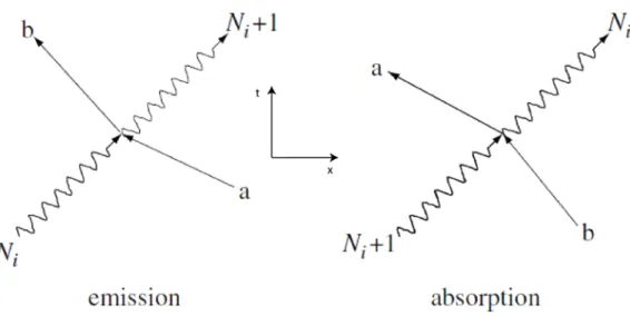
The simplest way to represent both of these interactions is using Feynman diagrams. These diagrams are pictorial representations of the mathematical expressions that rule the behavior of subatomic particles and, since those interactions can be complex and hard to understand, the Feynman diagrams allow us to simplify them. Figure 1 shows two simplified Feynman diagrams of the absorption and emission processes.

Figure 1 – Simplified Feynman diagrams for the emission (felt) and absorption (right) of a photon by a bound or free electron.

In the previous figure, the wavy lines represent photons with Ni being their number before the

interaction and the straight lines represent free or bound electrons with initial and final state denoted by a and b respectively.

The emission diagram (Figure 1, left) covers both the spontaneous and stimulated emission processes, generating a new photon and an electron loses the corresponding amount of energy in the form of kinetic energy if it’s a free electron; or potential energy if the electron is bound to an atom or a molecule. This change of potential energy usually occurs in discrete increments since these bound electrons exist in a discrete spectrum of Eigen states of the atom or molecule and the required momentum to generate the photon spin is also given away or taken up by the electron. If the number of photons before the interaction is zero (Ni=0), a photon can still be emitted in a process known as

spontaneous emission and, since there no photons, it is considered that the electron is interacting with a randomly fluctuating electromagnetic field that covers all space. In the QED model, the continuous creation and almost simultaneous destruction of virtual particles, electron/position pairs, is the reason for the arising of the vacuum fluctuation field and, although they are simultaneous events, denying us the possibility of measure those virtual particles, we can calculate and measure their secondary effects. The most significant of these events is the spontaneous production of radiation by excited atoms and molecules and it’s the source of all radiation occurred naturally and most of light made by man. In the case that there are already photons before the interaction (Ni>0), these will interact with the electrons

through a process called stimulated emission, like we see in lasers, and it’s tied to a fundamental property of the photon, its integer spin. Assuming we have a probability per unit time, p, for the creation or scattering of a photon in an empty final stage of the field, then we will also have the

containing Ni photons and since there’s a high probability for a photon to hit an occupied state, we can

establish situations that favor the increase the number of photons.

The absorption diagram (Figure 1, right), with Ni+1 photons in one initial state shows the interaction

with an electron, resulting with the absorption of one of them leaving Ni photons in the final stage of

the field. This diagram is the time-reversed diagram of the emission process and it can be shown that, like their classical electrodynamics counterpart, the equations of QED are symmetrical in time obtaining identical results under time reversal. Using the previous analysis of the stimulated emission probability, we can conclude that the probability of absorption of a photon from a state of the field containing Ni+1 photons is (Ni+1)p. after absorbing the photon, the electron will gain kinetic energy if

it’s already moving freely in space, or potential energy if it’s bound to a nucleus.

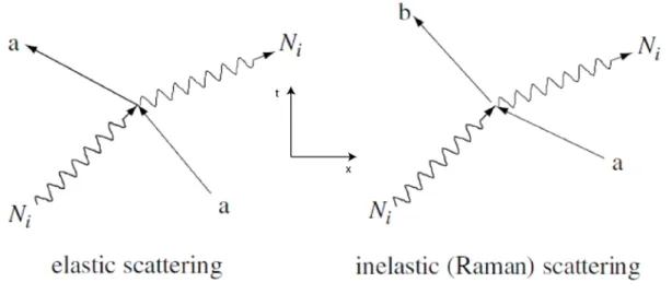
1.1.2 Scattering

One thing that the previous interactions have in common is that the final state of the field is the same as the initial, varying only the number of photons and the state of the electron. If a photon is absorbed and immediately re-emitted and the fields and electron states change we have a new kind of interaction called scattering. We can also divide that kind on interaction in two sub kinds, elastic and inelastic scattering pictured in simplified Feynman diagrams on figure 2.

Figure 2 – Simplified Feynman diagrams for the elastic scattering (felt) and inelastic scattering (right) of a photon by a bound or free electron.

When the outgoing photons have the same energy than the incoming ones, we have a kind of interaction denominated elastic scattering (figure 2, left) and the electron that participated regains the momentum value for the law of momentum conservation to be fulfilled. In other words, the state of the incoming photon changes as well as the direction of motion of the electron to account for the

momentum exchange. However, the bound state of the electron does not change. This interaction is also the most frequent photon-electron interaction in nature and there are two interesting features of the QED solution for it: at low energies, where we can ignore the relativistic effects, the angular pattern of scattered photons is identical to the dipole scattering pattern first derived by Rayleigh and Thompson [31]; and each photon that is scattered has a delay in which shows itself as a phase difference between the incoming and the scattered light waves.

If there is an energy difference between the incoming and the outgoing photons after an interaction, a different kind of scattering occurs: the inelastic or Raman scattering.

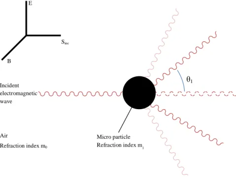
Most objects that we see are visible due to light scattering from their surfaces making it our primary mechanism of physical observation [32] [33]. Scattering of light depends on the wavelength or frequency of the light being scattered. Since visible light has wavelength on the order of a micrometer, objects much smaller than this cannot be seen, not even with the aid of a microscope [31].

Figure 3 – Schematic representation of light scattering.

The interaction of light with matter resulting in scattering can give us important information about physical properties like the structure and dynamics of the samples. If the scattering centers are in motion, the scattered radiation is Doppler shifted and an analysis of the spectrum of scattered light can yield information regarding the motion of the scattering center. Another property that causes the spectrum of scattered light to change is the periodicity or structural repetition in the scattering medium. All these physical results allow us to have information about the structure, spatial

E B Sinc θ1 Air Refraction index m0 Micro particle Refraction index m₁ Incident electromagnetic wave

configuration, or morphology of the scattering medium by studying the scattered light intensity as a function of the scattering angle [34].

The differential scattering cross section describes the power scattered per unit solid angle, for an incident intensity value:

Ω = Ω sca sca P I d dC 0 1 (6) With:

Ω

d

dC

_sca

– differential scattering cross section, [m2/sr];

0

I

– incident intensity, [W/m2];

sca

P

– power scattered, [W];

Ω

– solid angle, [sr].

The scattered intensity is the scattered power per unit area of detection:

A

P

I

sca

sca

=

(7)

With:

I

_sca – scattered intensity, [W/m2];

A

– area of detection, [m2].

The solid angle subtended by a detector at a distance from the scattering source can be given by:

2

r

A

=

Ω

(8)

With: r – distance from the scattering source, [m].

Combining equations (7) and (8) we obtain:

2 0

1

r

d

dC

I

I

sca sca

=

_Ω

(9)

This equation contains the well know dependence with 1/r2 due to the three dimensional geometry of space. We can also note that the intensity of the scattered light is directly proportional to the differential cross section.

The total cross section is found by the integration of the differential cross section (6) over the entire solid angle:

Ω

Ω

=

∫

d

d

dC

C

sca sca _4π (10)

Although we are able to study different physical and chemical properties with light scattering, doing it all and in detail takes time and, since our ultimate goal is to identify each particle, we can conclude that it’s impossible doing it in real or useful time using only this technique. At the end, it was decided that the study of light scattering would only be used to detect a particle and its preliminary analysis. The particle detection is made when light scattered is detected and the preliminary analysis measures the size, speed and the shape of the particle. Both the speed and the shape determination use features from the system and only the size requires a deep study on the field of light scattering.

While studying light scattering, depending in the variable that is used to collect the light, two different techniques can also be used: time dependent, also known as Static Light Scattering; or intensity dependent also known as Dynamic Light Scattering [35].

Static light scattering measures the intensity of the scattered light for a defined period of time with or without an angular dependency, obtaining the mean square fluctuations. It provides precise information on size and shape and for the results to be precise, the samples must have the least movement possible, allowing the time period to be maximum [36]. It is commonly used to determine molecular weight of macromolecules; the radius of gyration also known as the root mean square radius by measuring the scattering intensity on an angular range; and the second viral coefficient by measuring the scattering for different concentrations [37] [38] [39] [40].

Dynamic light scattering also has a time dependency but, during that time, it will obtain the scattered light in real time, instead of only obtaining the mean value. While a particle is crossing a laser beam, the intensity of the scattered light changes and it’s this value that is studied with this technique. Analysis of these intensity fluctuations enables the determination of the distribution of diffusion coefficients of the particles, which are converted into a size distribution using established theories [41].

Figure 4 – Plot comparing both techniques, SLS and DLS. For SLS, it’s the mean between [0, 10] ns.

The previous plot shows what we measure for each technique and each one has a broad range of applications. While they are usually used separately, they can also be used together [42]. The experiment that will be described is one of these examples, with the difference that, instead of using one technique after the other, it uses both at the same time, taking some advantages of each one.

In the case of the spherical particles, there are three different approaches to study the scattering effect depending of the particle size:

• Particles with diameter

D

>>

λ

_inc – Geometrical Reflection/Refraction; • Particles with diameter

D

≈

λ

_inc – Mie Theory;

• Particles with diameter

D

<<

λ

_inc – Rayleigh Theory.

1.1.3 Geometrical Reflection/Refraction (

D

>>

λ

_inc

)

With this effect, the incident light is partially reflected and refracted from medium interfaces in many directions. This can be taken into account by defining the complex index of refraction:

[ ]0,1 n[ ]0,1 ik[ ]0,1

m = − (11)

k

– the imaginary part, indicating the amount of absorption loss.

Some part of the energy is also absorbed and dispersed in a non-radiative way inside the particle. Due to symmetry (in the case of the spherical shape), the scattering and absorption from the particles is uniform for the same

θ

, which is not more the case for non-spherical particles. The scattering pattern (angular dependence of scattered light intensity) becomes much more complicated, but at the same time it can provide additional information on the particle shape. At the end, finding the corresponding scattering pattern for each geometrical shape is a complex ray tracing problem and to overcome this, the common approach is to measure the pattern for some well-defined particles shapes and to investigate how the data changes with different samples [43] [44].

This approach was not used since there wasn’t enough time to try or test particles of this size range. In the future, a bigger focus will be given to this study, since our ultimate goal is to measure the broadest size range and for bigger particles, this kind of interactions has a major contribution.

1.1.4 Mie Theory (

D

≈

λ

_inc

)

For particles with sizes comparable or smaller than the wavelength, the total cross section (called also extinction cross section) describes the efficiency that gives amount of incident energy lost on scattering and absorption:

Ω Ω = d d d I F ext inc ext

σ

(12)

With:

d

Ω

– solid angle given by

d

Ω

=

sin

( )

θ

d

θ

d

φ

, [sr]; ext

F

– extinction of the radiant flux through the solid angle, [W];

inc

I

– incident intensity, [W/m2];

ext

σ

– total extinction cross section, [m2].

The total extinction cross section is expressed by:

scat abs

ext

σ

σ

σ

=

+

(13)

In Mie theory, the differential scattering cross sections for the vertical and horizontal polarizations are defined by the following expressions (case of the spherical particles):

( )

θ

π

λ

θ

σ

1 2 2

4

S

d

d

_V

=

(14)

( )

θ

π

λ

θ

σ

2 2 2

4

S

d

d

_H

₌

(15)

With:

S

₁

( )

θ

,

S

₂

( )

θ

– angular scattering amplitude functions, [dimensionless];

λ

– wavelength, [m].

These functions are derived as following:

( )

₍

₎

(

( )

( )

)

2 1 1 cos cos 1 1 2

_π

_θ

_τ

_θ

θ

n n n n n b a n n n S + + + =

∑

+∞ = (16)

( )

₍

₎

(

( )

( )

)

2 1 1 cos cos 1 1 2

_τ

_θ

_π

_θ

θ

n n n n n b a n n n S + + + =

∑

+∞ = (17)

With:

a

_n,

b

_n – parameters defined with Ricatti-Bessel functions, [dimensionless];

n

π

,

τ

_n – functions expressed in terms of Legendre polynomials, [dimensionless].

The total extinction and scattering cross sections can be then derived as follows [45]:

(

)

(

2 2

)

1 2 2

1

2

2

n n n scat

=

∑

n

+

a

+

b

+∞ =

π

λ

σ

(18)

(

) {

_{n n}

}

n ext

=

∑

n

+

a

+

b

+∞ =

Re

1

2

2

2 ₁ 2

π

λ

σ

(19)

As we can see, these equations are not particularly simple to use or to gain physical insight. It gets ever worse if we see some examples of the Mie scattering for spheres with a variety of sizes:

Figure 5 – Normalized Mie scattering curves [46].

The previous plot shows some normalized Mie scattering curves as a function of scattering angle for spheres of refractive index m=1.50 and a variety of size parameters α=ka, with a = radius and k = 2π/λ. The intensity is normalized, I(θ)/I(0) and a series of bumps are seen with some periodicities, but with no particularly coherent pattern. It was important to understand well this kind of interaction since it was the only one used in our system. At the end we were able to use a MATLAB simulation that helped us to determine the curves for all the sizes that we used [47] [48].

1.1.5 Rayleigh Theory (

D

<<

λ

_inc

)

Rayleigh approximation allows us to define the differential scattering cross sections for the vertical and horizontal polarizations in a shorter way:

2 2 2 2 6 2 1 1 4 + − = m m d d V

π

α

λ

θ

σ

(20)

( )

θ

σ

_θ

θ

σ

d d d d _H 2 _V cos = (21)

α

– size parameter,

λ

π

α

= 2 D, [dimensionless];

D

– Diameter, [m].

For the total absorption cross section, the expression is following:













+

−

−

=

1

1

Im

₂ 2 3 2

m

m

abs

_π

α

λ

σ

(22)

Finally, for non-polarized light the extinction cross section can be written as:

2 2 2 6 2 1 1 3 2 + − = m m scat

_π

α

λ

σ

(23)

Once again, this approach was not used since we didn’t analyzed any particles that were smaller that the laser wavelength. It will be also a future feature to be able to detect this range of particle sizes.

2. System Description

This system was meticulously developed by Dr. Kiselev for its Ph.D. thesis [49]. Everything was made from scratch, including all the circuit designs and most of the pieces. While thinking of this project as a flexible one instead of a fixed one, there was room for improvements and at the end, practically everything is different from the original design. Even now, while writing this report, we are thinking of ways to improve the system. These changes were not just in terms of physical appearance but also the way it works so, instead of showing the modifications, this chapter will explain all parts of the system, including how they work and their purpose, how the data is collected and processed and how the calibration was made.

2.1 Metrologic Model

This main objective for the development of this system was to determine the size, in real time, of a micro particle by analyzing its scattered light. Not only that, but by analyzing the time that took the detection since when it stared until when it ended, we would be able to determine the speed of the same particle. This was our method under test.

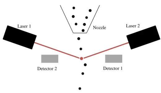
The main idea is: Create a thin airflow and, at a certain point, illuminate with light coming from red lasers on one side and obtain the scattered light with light detectors. A scheme of this idea is on figure 6:

Figure 6 – Schematic of the system.

To be able to correlate the data of this system, a calibration method was also developed using Mie

Laser 1 Laser 2

Detector 2 Detector 1

2.2 The System

The idea was developing a device ready for in-field experiments and at the same time ready for coupling with other techniques or detection methods. Instead of a typical laboratory assembly that could occupy a whole optical table, since the beginning that a more compact system was though and the main pieces were designed by Kiselev, some minor ones by me and made by the Mechanical Workshop of the University of Geneva or the small Mechanical Workshop at the Group of Applied Physics.

The priority requirements of the detector were:

• A hermetic system for the air flow generation between the two air entrances and the exit. This is important because the efficiency of the detections is better without leaks and, since we have two air entrances, this importance is even higher due to the fact that both need to have the same flow. Another important aspect is, for a detector of this kind to work without malfunctions on the field, it is very important that no humidity or other kind of particles enter inside it so while the detector box is hermetic, we will have the air flow generation inside, another hermetic system.

• A chamber with the ability to have multiple windows for both input and output of the different light/excitation sources. Like we will see later, the chamber is the most important piece of the detector because it is where the interactions between the particles and the lasers happen. Such interaction must be well observed since all the results will come from here.

Analyzing these priorities we can see that other than the hermetic chamber with the air flow, the rest of the components can be placed anywhere since we can user mirrors and cables to transport the light and electrical signals respectively.

The final design is shown on the figure below; we’ll discuss each part in more detail afterwards.

2.2.1 Aerosol Flow Generation

For this system to detect something, it needs a proper kind of flow so, when the air flow enters the chamber, it needs to be thin and laminar. These aspects are important if we want both lasers to hit each particle, in fact we can actually say that this part is one of the principal parts of the detector since the results depend of the quality of the air flow. Different designs of nozzles were tested, before the elaboration of this work, from single inlets to double inlets and different materials [49].

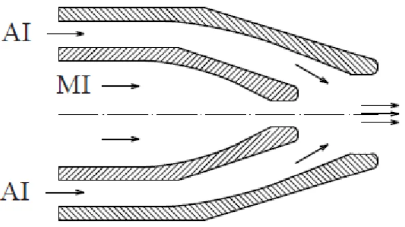
Figure 8 – Stealth nozzle geometry scheme: MI – main inlet; AI – auxiliary inlet.

The used nozzle has a Stealth Nozzle geometry, producing a thin and long laminar flow and its design was inspired by the geometry proposed by Prof. R. K. Chang and his colleagues [50]. The material chosen for the nozzle is nickeled brass because it is easy to machine like aluminum, but less fragile, and has a very high surface quality.

Figure 9 – Nozzle parts [49].

its high performance allows us to change each axis with great precision. To move the nozzle on the Z axis, another piece was created. That piece connects to assembled piece shown on figure 5 and is has a helical ridge where is a washer screwed. Rotating more or less the washer will adjust the height of the nozzle until the best result is achieved. The washer is then fixed on the top of the translation stage.

The bottom of the chamber is connected to a pump that sucks the air from both inlets. This pump has the characteristics indicated on table 1.

Table 1 – Pump characteristics.

Manufacturer KNF

Model N 86 KNDCB

Operating Voltage (VDC) 12

Delivery at atm. Pressure (l/min) 6

Max. operating pressure (bar g) 2.4

Ultimate vacuum (mbar abs.) 100

This model was chosen for its compact size and possibility to have its filters changed quite easily.

2.2.2 Light Sources and Scattering Detection

In order to have light scattering signals, a light source, a photo sensible sensor and the sample to be analyzed are needed. The last one was discussed previously, the samples come directly from the nozzle. The light source come from two red lasers and the photo sensible sensor is a PMT, in this case two PMTs are used. I will describe in more detail each one of this parts next and where it’s done.

2.2.2.1 Red Lasers

For light scattering to occur, usually a laser is used as a light source. For this system two special lasers were used. Instead of using two continuous lasers like it was described on the previous designs [49], a new technique was developed using two modulated lasers at 2 MHz. This technique will be described later and for it to work, two modulated lasers are needed. The characteristics of the chosen lasers are on the following table:

Table 2 – Lasers characteristics.

Manufacturer Power Technology Incorporated

Model IQ1A

Operating Voltage (VDC) 5 - 15

Emission Wavelength (nm) 690

Max. Output Power (mW) 30

Operating Temp. Range (°C) 5 - 40

Max. Operating Current (mA) 3000

Mod. Current Above Bias (mA) 10 - 1000

Modulation Freq. Range (MHz) CW - 70

Beam Divergence (1/e2_{, mrad) <1}

Rise/Fall Time (ns) 10

Propagation Delay (ns) 20

This model was chosen especially for its ability to be modulated at the frequency that we want to work (2 MHz) and also for its emission wavelength, 690 nm. Being an analog modulated laser, another technique that will also be described later uses a control voltage correction, allowing us to change the output power of the laser. The ability to be modulated with different intensities made this laser the perfect solution for this system.

2.2.2.2 PMTs

The sensor that was chosen for light collection was a photomultiplier H10720-20 from Hamamatsu Photonics. The characteristics of this module are given in the following Table:

Table 3 – PMTs characteristics.

Manufacturer Hamamatsu Inc.

Model H10720-20

Spectral Response (nm) 230 – 920

Input Voltage (V) +4.5 to +5.5

Max. Input Voltage (V) +5.5

Max. Input Current (mA) 2.7

Max. Output Signal Current 100

Max. Control Voltage +1.1 (1MΩ)

Recommended Control Voltage Adjustment Range (V) +0.5 to +1.1 (1MΩ)

Effective Area (mm) ϕ8

Peak Sensitivity Wavelength 630

Cathode

Luminous Sensitivity Min. (μA/lm) 350

Typ. (μA/lm) 500

Red/White Ratio Typ. 0.45

Radiant Sensitivity Typ. (mA/W) 78

Anode

Luminous Sensitivity Min. (A/lm) 350

Typ. (A/lm) 1000

Radiant Sensitivity Typ. (A/W) 1.5 x 105

Dark Current Typ. (nA) 10

Max. (nA) 100

Rise time (ns) 0.57

Ripple Noise Max. (peak to peak) (mV) 0.3

Settling Time Max. (s) 10

Operating Ambient Temperature (°C) +5 to +50

Storage Temperature (°C) -20 to +50

Weight Typ. (g) 45

This sensor has its peak sensitivity on the wavelength of the lasers that we use, providing high sensitivity and high speed response since its rise time is low. It makes it ideal for scattering light measurements and with suitable electronics and changing the gain settings, it allows us to change the sensibility and the noise.

2.2.2.3 The Chamber

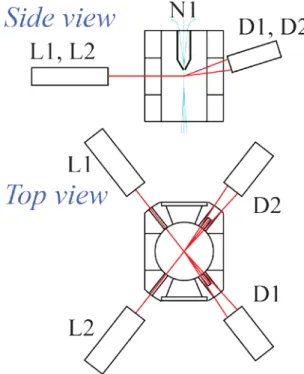
The chamber is where all scattering physical interactions happen and it was organized to provide easy access and adjustment mechanisms for all components, and to allow integrating new components for further experiments. The scheme of the measurement chamber is shown on the following figure:

Figure 10 – Chamber scheme.

The elements are positioned as following:

• two red lasers (L1, L2) are placed in the horizontal plane 1 - 2 mm lower than the nozzle outlet;

• the angle between the two lasers is about 100°

• both laser beams are blocked by beam dumps inside the chamber;

• each detector (D1, D2) is placed in front of the corresponding laser and tilted in the vertical plane by around 19°. Its field of view is therefore directed on the intersection of the red lasers but tilted out from the laser axis;

2.2.3 Electronics

Besides the PMTs (D1, D2) and the Lasers (L1, L2), the electronic part of the system also consists of two analogue to digital conversion modules (AD1, AD2), two digital to analogue conversion modules (DA1, DA2), one field programmable gate array (FPGA) (PL), and one embedded computer (EC). These last two will be described later and the conversion modules are the bridge between the detectors and lasers with the field programmable gate array, allowing it to read the data from the detectors and change the laser parameters, according to the next figure:

Figure 11 – Electronics scheme.

The way the whole system works will also be explained later. The whole system could have been simpler but, since our aim was to build it flexible, adaptive and always looking for improvements, the final version ended with a lot more components that the prototype one [49].

2.2.3.1 The Embedded Computer

The heart of the system is its own embedded computer. Although it seems more complicated that the traditional approaches, which usually involve an external computer and making it harder to retrieve the data, having its own computer simply simplifies a lot its configuration, the data retrieval and even remote access. A full computer with an operating system, in this case Linux, allows us to change the detector parameters, access the data and even do a first data processing without the need of another computer, simplifying the procedures to do different detections.

Table 4 – Embedded computer characteristics.

Manufacturer Toradex

Model Robin Z530 L

CPU Name Intel® Atom™ Z530

CPU Type x86

CPU Cores 1x

CPU Clock 1.6 GHz

Threading Hyper Thread

Instruction Cache 32KByte

L1 Cache 24KByte

L2 Cache 512KByte

RAM 1 GB DDR2 533 MHz

Flash 4 GB SSD on IDE

PCIe 1 x1

USB Host & Device 7 x USB 2.0 (1 channel configurable as device)

I2C 1x (via USB Controller)

GPIOs 8 x GPIO (via USB Controller)

Ethernet 10/100/1000 Mbit

ExpressCard supported

Serial ATA 1 x Serial ATA (via IDE Bridge)

SDIO/SD/MMC 2 x SDIO (4/8bit), MicroSD slot on module

LPC 1x

SMB 1x

Controller Hub Intel® System Controller Hub US15W

Display Controller Dual, Independent

Graphics Controller Integrated Intel® Graphics, Intel® GMA 500, HDTV/HD capable

Video Decoder Decoder for MPEG2 / HD / H.264

LVDS LVDS Single Channel 18/24 bit WXGA 1366x768

SDVO 2048 x 1152 on request

VGA 1920 x 1080

HDA 2x

Operating Systems WinXP, WinXP Embedded, WePOS, Win7, WES7, Windows CE6, Linux

BIOS Award

Size 84.0 x 55.0 x 10.8 mm

Temperature 0° to 60° C

Power Dissipation 4.7 - 6.9 W

Minimum Availability 2017

A quick look through this table reveals us most of the normal components existing in desktops or in laptops. The reasons this model was chosen are the compact size, allowing us to have more freedom to place it along with the mechanical parts, the CPU characteristics, since this model (Intel Atom) is everywhere, from ITX desktops to laptops and netbooks and with our objective to install an operating system on it, this CPU has an huge Linux community support, allowing us to find help easily; and, maybe the most important feature in this embedded computer model, is the PCI Express feature.

Unlike netbooks or some laptops, the PCI Express port does not exist and for this project was really important since it’s the only port where the FPGA (PL in figure 7) can be connected.

2.2.3.1 The Field Programmable Gate Array

Using the same analogy, the brain of this system is a FPGA which is connected to all components of the system. It’s the FPGA that receives the data from the detectors and with it, is able to control the intensity of the lasers, a process that will be described in the next subchapter.

Table 5 – FPGA characteristics.

Manufacturer Enclustra

Model Mars MX2

Form Factor SO-DIMM (68 x 30 mm)

Connectors 200-pin SO-DIMM

FPGA Xilinx Spartan-6 LXT

Memory •Up to 256 MByte DDR2 SDRAM

•Up to 16 MByte quad SPI Flash

User I/O 108 FPGA I/Os, single-ended or differential

Interfaces •PCIe x1 endpoint

•Gigabit Ethernet

Supply Voltage 3.3 V

This model was chosen since it’s a Xilinx Spartan, one of the most known FPGA’s ever and it’s a compact SO-DIMM form factor.

2.3 Data Measurements

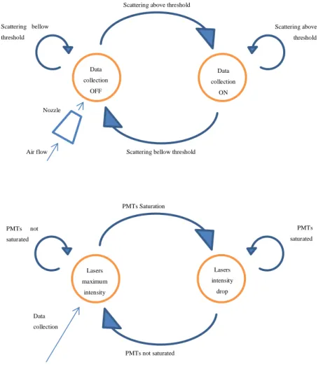
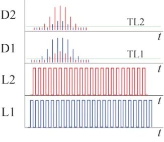
The simplest way to explain how this system works is by using state machines. There are two completely independent state machines, one for the detections and other for the laser intensity adjustment and both are always active. They are shown on figure 10 and each one will be described in detail.

Figure 12 – State machines for the data collection (up) and the lasers intensity adjustment (down).

The lasers are intersected in the middle of the chamber on the air flow close to the nozzle outlet. The lasers (L1, L2) are the same model, each one oscillates with at 2 MHz repetition rate, and the phase offset between both is constant and equal to 180°. In this way, there is always only one of the lasers switched on while the second one is not emitting. Both detectors (D1, D2) are supplied with a dedicated narrow band pass filters centered at the laser wavelength. This makes the detection system completely symmetric and allows the equivalent scanning of individual particles in the vertical direction from two sides. Moreover, each detector is able to see both lasers but with on the different scattering angles (15-23° and 106-114°) and the system only starts to collect data after the intensities pass the threshold value (TL1, TL2).

Scattering above threshold

Scattering bellow threshold

Scattering above threshold

Scattering bellow threshold Data collection OFF Data collection ON Air flow Nozzle PMTs Saturation PMTs not saturated PMTs saturated PMTs not saturated Lasers maximum intensity Lasers intensity drop Data collection

Figure 13 – Detection cycle.

Like was described previously, this laser model allows us to change the intensity output according with the input so this system has another feature: it has the ability to avoid the detector saturation by reducing the laser intensity. It is based on a rapid digital feedback circuit that regulates laser (L1, L2) amplitude for each laser shot. When the laser control voltage is 1V, it will have a 100% power output and if the control voltage is 0V, it will have a 0% output.

Figure 14 – Detection cycle with amplitude regulation.

We know beforehand that the relationship between voltage and output power is not linear [51] and, for this adjustment system to work, first we need to know exactly how the laser output change according with the input, or in other words, we need a calibration curve for each laser. To achieve it, we manually set the laser intensity values, analyzing the output using a normal photodiode and an oscilloscope. There was no need to study the photodiode with much detail since only the intensity will change, making the beam continuous and maintaining the wavelength. We decided to make 17 measures from 0V to 1V obtaining the following values and its corresponding plot:

Table 6 – FPGA characteristics.

Input Value

(mV) _{Laser 1} Output Value (mV) _{Laser 2}

0 0 0 62.5 19 54 125 208 233 187.5 255 268 250 277 291 312.5 297 311 375 317 330 437.5 342 354 500 428 442 562.5 500 515 625 526 537 687.5 543 549 750 552 561 812.5 561 562 875 562 569 937.5 564 573 1000 563 570

Figure 15 – Plot with the output value in function of the input voltage for both lasers..

Since we want a linear correlation because it’s easier for the system to compute, especially in real time where you need a fast detections and analysis, the first thing we need is the symmetrical plot with the line between the lowest values and the biggest for each laser. Doing this will allows us to know what will be the values to add each point to make it linear.

0 100 200 300 400 500 600 0 200 400 600 800 1000 O ut put V al ue (m V) Input Voltage (mV) Laser 1 Laser 2

Figure 16 – Figure 15 with symmetrical plots..

Knowing this value difference dependence with the input allowed us to reach the most important part of this adjustment system: the adjustment itself. Forcing this linear dependence allows us to simply correct the values adding or subtracting values. Using equation (9) and knowing that the scattered light intensity depends mainly on the size of the particle and the intensity of the light input, we just change this last value and correct it on the data processing. At the end, we will have an expression like the following:

( )

1 1 max + + × = A A I I m c sca sca (24) With: c sca

I – Corrected scattering intensity value, [W/m2];

m

sca

I – Measured scattering intensity value, [W/m2];

A – Step values to change the laser intensity,

0

=

0

V

,

max(

A

)

=

1

V

, [dimensionless].

We add 1 in each part of the fraction because the step value can be zero, returning an error while trying to divide by 0. With this equation we are able to know, even with the correction algorithm, the scattered intensity value. Every time when the detector sees its signal increasing, the amplitude of the

next laser shot will be reduced by the amplitude step defined from the actual signal value. If the signal decreases, the laser intensity will go back until it reaches the maximum value. Our only limitation is step value and in this system, all inputs/outputs are controlled by the FPGA. It was decided to use 6 bits since it gives us enough values (64) and with the laser activity bits (2) makes a word or 8 bits. The laser intensity is represented as a set of values from 0 to 63, each one corresponding to 0V and 1V respectively. Using the calibration values shown on table 6 we were able to determine what is between these frontier values shown in the next table and figure:

Figure 17 – Input laser voltage in function of the decimal input value.

By inserting these values on the detector, we can finally use a linear dependency like on equation (24) but with well-defined values. The final output value of both detectors in this system is calculated according the formula:

1 64 + × = A I I m c sca sca (25)

2.4 Data Analysis

This system reads data from both detectors even during the laser oscillation while it’s off. This allows us to measure the scattered light in both detectors from each laser. This is important since we can

The raw data of the linear combination of the detectors and lasers results in four distinct trace shown on figure 18.

Figure 18 – Timely resolved scattering traces (upper figures).

On the left side of the previous picture we have the intensity seen by the detector 1 (D1) displaying the traces from both lasers (L1 and L2). These values already have the laser correction but they are not yet ready for the analysis. First the traces from the same detector (D1 or D2) are multiplied and smoothed by the moving average method (Figure 19).

Figure 19 –Product of scattering traces for each detector (lower figures).

Looking at the previous plots, we can see that the noise is low and only the important data remains. We first determine the maximum in each plot (M1, M2) and right after we find the time that the particle

took to cross the beams (t1, t2). The peak determination is first since the time interval is measured 95%

below the peak to avoid the inclusion some lower oscillations that could induce more errors. We also use these time values to calculate the integral of the curve (I1, I2) and these are the integrals that are

going to be used to determine the size of the particle. Different integral values correspond to different sizes since a bigger particle would take more time to cross the beams, raising the integral values. Contrarily, a smaller particle would take less time.

The time that the particle takes to cross the beams is also important for another determination, the speed. Knowing the speed is important if we want to shot the particle with another excitation source, like an UV laser to detect fluorescence or other or even more than one. For this we need to know in which speed is the particle moving to calculate when to shot the various excitation sources.

The last measure that we can do is the shape estimation of the particle and this system does it by comparing the values from the detectors, namely the integrals determined with the data from each one. If the particle is a sphere or has a symmetrical shape, the integral values should be the same. But, if the values are different, each integral has a different value, meaning that the data collected from each detector is different, giving us a non-spherical particle.

2.5 Calibration of the System

To be able to correlate the acquired data with the real values and before extracting any kind of results from this experience, we need to calibrate this system. Being a completely new system, we first need to have a known and well defined input and extract the output. To do this, commercial well defined size particles were used, as a powder or diluted in a liquid solution and two types of particle generators were used.

2.5.1 Micro Particles

In order for the calibration to be well done, we need a set of particles with different sizes but that size value must be quite precise. We used two different sets: The first one has ten different sizes with ranging from 1.5 μm to 10 μm and the second set has five sizes, from 11.6 μm to 31.3 μm. Each set’s mean sizes are displayed on the following tables:

Table 8 – [11.58, 31.3]µm specifications.

These particles were chosen since we wanted a big range of sizes do calibrate this device. We gave more importance to smaller sizes since it’s where we thought that the system was less sensitive. They could also be dissolved in water or we could use them directly as a high concentration power and we decided to use both.

2.5.2 Generators

Being on a liquid solution or in a high concentration powder, the particles weren’t prepared to go directly to the detector. To circumvent this, special particle generators were used, one for small particles and other for bigger particles. Using both generators was important since liquid solutions only work for the small particle generator and this generator can’t generate big particles. The liquid solution could allow us to use a low concentration of particles in water, giving a low number of detection per minute. This way the system wouldn’t saturate. Another problem is that the big particle generator can’t generate single small particles. The movement of it makes it difficult to generate just one particle, so they will come in bunches instead of one at a time.

2.5.2.1 Generation of small size aerosols

(

d

≤

2

µ

m

)

To generate small size aerosols, a commercial available system was used. Its main characteristics are shown in the following table:

Table 9 – Generator characteristics.

Manufacturer TSI Corp

Model Aerosol Generator 3076

Cut-off size (μm) 2

Flow rate (l/min) 3

Maximum particle concentration (particles/cm3_{) 10}7

The generation system contains three main parts shown in Figure [FIGURE] • air drying tube and filters (TSI Filtered Air Supply 3074);

• atomizer TSI Aerosol Generator 3076; • drying tube for outlet (custom made).

The drying tube for outlet uses silica drying crystals (BASF cat.num. : 54097617)

Figure 20 – Small size aerosol generator.

The main problem of this generator is that its maximum size is 2 µm and looking to the particle sizes that we have, only two measures were made with this one.

2.5.2.2 Generation of large size aerosols

(

d

≥

2

µ

m

)

Since the particles size range surpasses the maximum size of the first generator, we needed another one. A more simple solution was found, a homemade generator with a laboratory bottle with two holes: one on the top, being one of them for the input of the external air and the other for the output,

Figure 21 – Large size aerosols generator scheme.

The particle powder is placed inside the bottle and with the help of a nut and while shaking it, the powder with muck less concentration can reach the height where is the air flow made between the input and the output.

2.5.3 Calibration

To evaluate the capability of the system of size and speed measurement, the imaging of the Mie scattering patterns was done on the spherical silica beads. To do so, an amplified CCD camera (CCD), coupled with an objective, and a pulsed Nd:YAG laser (L3) were coupled with the system. The angular view of the objective is between 60° and 115°, using the laser optical axis as a reference and these values will be used to the Mie patterns simulation. The experimental scheme is shown on the following figure:

External Air

Figure 22 – Calibration scheme.

If a particle crosses the intersection of the lasers (L1 or L2) the system detects its presence, measures the size and the speed, and triggers the camera (CCD) and the laser (L3). As result, one snap shot is obtained on the camera for each detection event. It contains two images corresponding to two laser shots.

Using this scheme, we took snapshots for different particle of all the sizes available. Two examples are given on figure 24 for two different particles sizes, 6 µm and 25 µm respectively:

Figure 24 – Mie scattering patterns acquired with CCD camera: a) particle of 6 µm; b) particle of 25 µm.

Looking at the previous snapshots, the first thing that is noticeable is the cross with an inner circle. This strange shape belongs to the objective: the inner circle corresponds to the inner mirror also known as second mirror and the cross lines are the support for that mirror. While trying to quantify the snapshots, we can distinguish three different variables: The diameter of the circle (D), the distance between two circles (L) and the number of colored lines and each one will be explained, starting by the last one.

The colored lines represent the Mie scattering pattern and what we actually see can be represented by the curves on figure 5. To have a better understanding of these snapshots, a MATLAB simulation was used [47] [48], having the same input parameters as our system and there are two different plots: one for all angular range, from 0° to 180° and the second one to the angular view of the objective, from 65° to 115°.

Figure 25 – Mie scattering patterns from the MATLAB simulation: left) [0°, 180°]; b) [65°, 115°], corresponding to the field of view of the objective.

The previous plots differ from the one mentioned on the introduction because they are not normalized but we can see the same curved shape for different sizes. For the 6 µm we can see that the number of peaks is the same both in the snapshot and in the simulation (7 peaks). For the 25.6 µm it’s more difficult to compare both values, but possible. We can also explain the intensity difference as a function of the angle, for smaller angles we have a bigger intensity, and that’s the reason why we have a color difference in the snapshots, almost saturating on the left side and getting darker on the right. By doing this measurement for all particle sizes existing in the lab and confirming them analyzing the snapshots, we were able to correlate the particle size with the integrals measured by the system. Another important feature that we can extract from these snapshots is that we are detecting single particles. With both generators we cannot have any certainty that we are generating single particles but, since the Mie theory only works for spherical particles, having more than one would change the shape and consequently the Mie patterns would be completely strange. An example of that is on the following snapshot: