i
MASTERS
FINANCE
MASTERS FINAL WORK
DISSERTATION
THE EFFICIENCY IN MARKOWITZ,
MINIMUM-VARIANCE AND NAÏVE PORTFOLIOS APPLIED TO
SMI
CRISTIANO MATEUS CUNHA FERNANDES
COMITEE MEMBERS:
PRESIDENT: PhD RAQUEL MARIA MEDEIROS GASPAR
SUPERVISOR: TIAGO RODRIGO ANDRADE DIOGO
MEMBERS: PhD JOÃO LUÍS CORREIA DUQUE
ii
MASTERS
FINANCE
MASTERS FINAL WORK
DISSERTATION
THE EFFICIENCY IN MARKOWITZ,
MINIMUM-VARIANCE AND NAÏVE PORTFOLIOS APPLIED TO
SMI
CRISTIANO MATEUS CUNHA FERNANDES
COMITEE MEMBERS:
PRESIDENT: PhD RAQUEL MARIA MEDEIROS GASPAR
SUPERVISOR: TIAGO RODRIGO ANDRADE DIOGO
MEMBERS: PhD JOÃO LUÍS CORREIA DUQUE
iii
A
bstract
This study aims to analyze various models of portfolio management, underlying the active and passive management and its impact on the efficient choice of an optimal portfolio composed by assets from Swiss shares index - SMI.
I chose Swiss market for a couple of reasons. First of all, it would be interesting to analyze the behavior of an European market that doesn’t belong to Euro. Another reason was the fact of this market have some big international companies such as Nestlé and Swatch.
Historical portfolio analysis took into account the Markowitz model (mean-variance), the Minimum Variance model and the Naïve model (equal weights). The time horizon used in this dissertation was 10 years and considers the period between January, 2004 and December, 2013. The data were obtained from academic database Datastream.
To compute the weight to invest in each asset, “data window system” for 1 and 2 years will be used.
To conclude, we will be able to see if, for 12 months, there are or not significant differences between the types of portfolio management treated throughout the dissertation. Further on, we may consider if for higher returns and Sharpe Ratio, the optimal portfolio is the best option.
JEL Classification: G11, G15
Keywords: Markowitz Portfolio Theory, Naïve Portfolio, Minimum-Variance Portfolio, Sharpe Index.
iv
Resumo
Esta dissertação tem como objectivo analisar vários modelos de gestão de carteiras, tendo em consideração gestão activa e passiva e o seu impacto na escolha eficiente de uma carteira ótima composta por activos do índice bolsista Suiço - SMI.
A minha escolha recaíu sobre a Suiça por várias razões. Em primeiro lugar, seria interessante perceber o comportamento de um mercado europeu que não utilizasse a moeda única. Outra das razões foi por este mercado incorpora algumas grandes empresas multinacionais, tais como a Nestlé e a Swatch.
A análise histórica das carteiras teve em conta o modelo Markowitz (média-variância), modelo Mínima-Variância e o modelo Naïve (pesos iguais). O horizonte temporal utilizado neste estudo foi de 10 anos, considerando o período de Janeiro de 2004 a Dezembro de 2013. Os dados foram retirados da base de dados académica Datastream.
Para calcular o peso a investir em cada ativo, foram utilizados os sistemas de “janelas de dados” a 1 e 2 anos.
Por fim, será possível observer se, para 12 meses, existem ou não diferenças significativas entre os modelos de gestão de carteiras estudados nesta dissertação. Será também possível analisar se, para rendibilidades e rácios de Sharpe mais elevados, a carteira ótima é a melhor opção.
Classificação JEL: G11, G15
Palavras-Chave: Teoria Carteira Markowitz, Carteira Naïve, Carteira de Mínima Variância, Índice Sharpe.
v
Aknowledgment
Masters Final Work was the most challenging task that I have had during all my academic life. To make this happen, I was strongly supported by some people that I would like to thank:
To Professor Tiago Diogo for all the help and support given during all this long
period. After being my teacher during my graduation, Professor Tiago Diogo was a huge help to discuss and to push me up to reach the success;
To my parents, for the support during all my academic and professional career.
Without them, I wouldn’t be able to the man I am and would never be strong enough to combine my professional and academic career;
To my brother and his wife, Tiago and Ana, for having always outstretched hands to
push me up, when I was feeling down, even being more than 1.500 km far from me, just like my parents;
And finally, to my girlfriend Ana Rita Bogas for all the support, friendship and love
given during all this time. I promised her that I would work hard to make her proud of me and my work.
1
Tables List
TABLE 1 – HYPOTHESES TESTS, WITH 1 YEAR “DATA WINDOW ... 23 TABLE 2 – HYPOTHESES TESTS, WITH 2 YEARS “DATA WINDOW ... 24
2
Figures List
FIGURE 1 – MARKOWITZ PORTFOLIO RETURNS, 1 YEAR “DATA WINDOW” ... 30
FIGURE 2 – MARKOWITZ PORTFOLIO SHARPE INDEX, 1 YEAR “DATA WINDOW” ... 30
FIGURE 3 – MINIMUM VARIANCE PORTFOLIO RETURNS, 1 YEAR “DATA WINDOW” ... 31
FIGURE 4 – MINIMUM VARIANCE PORTFOLIO SHARPE INDEX, 1 YEAR “DATA WINDOW” ... 31
FIGURE 5 – NAÏVE PORTFOLIO RETURNS, 1 YEAR “DATA WINDOW” ... 32
FIGURE 6 – NAÏVE PORTFOLIO SHARPE INDEX, 1 YEAR “DATA WINDOW” ... 32
FIGURE 7 – RETURNS COMPARISON OF BOTH 3 PORTFOLIOS, 1 YEAR “DATA WINDOW” ... 33
FIGURE 8 – SHARPE INDEX COMPARISON OF BOTH 3 PORTFOLIOS, 1 YEAR “DATA WINDOW” ... 33
FIGURE 9 – MARKOWITZ PORTFOLIO RETURNS, 2 YEARS “DATA WINDOW” ... 34
FIGURE 10 – MARKOWITZ PORTFOLIO SHARPE INDEX, 2 YEARS “DATA WINDOW”... 34
FIGURE 11 – MINIMUM VARIANCE PORTFOLIO RETURNS, 2 YEARS “DATA WINDOW” ... 35
FIGURE 12 – MINIMUM VARIANCE PORTFOLIO SHARPE INDEX, 2 YEARS “DATA WINDOW” ... 35
FIGURE 13 – NAÏVE PORTFOLIO RETURNS, 2 YEARS “DATA WINDOW” ... 36
FIGURE 14 – NAÏVE PORTFOLIO SHARPE INDEX, 2 YEARS “DATA WINDOW” ... 36
FIGURE 15 – RETURNS COMPARISON OF BOTH 3 PORTFOLIOS, 2 YEARS “DATA WINDOW” ... 37
FIGURE 16 – SHARPE INDEX COMPARISON OF BOTH 3 PORTFOLIOS, 2 YEARS “DATA WINDOW” ... 37
3
Contents
1 INTRODUCTION ... 4 1.1 PREAMBLE ... 4 1.2 PURPOSE ... 5 1.3 STRUCTURE ... 5 2 LITERATURE REVIEW ... 62.1 MARKOWITZ AND THE OPTIMAL PORTFOLIO ... 6
2.2 PERFORMANCE EVALUATION ... 14
2.3 CONCLUSION REMARKS ... 17
3 TESTING HYPOTHESIS ... 19
4 METHODOLOGY AND DATA ... 21
5 RESULTS ANALYSIS ... 25
5.1 OVERVIEW ... 25
5.2 HYPOTHESES TESTS RESULTS ... 26
6 CONCLUSIONS ... 28
6.1 MAIN CONCLUSIONS ... 28
6.2 LIMITATIONS ... 29
6.3 SUGGESTIONS FOR FUTURE INVESTIGATIONS ... 29
7 BIBLIOGRAPHY ... 30
4
1
Introduction
1.1 Preamble
The subject of this dissertation builds on the discussion of the various types of portfolios composed of financial assets. The focus of this thesis is based on the portfolio management. The opinions on what type of management is the best for investment in financial assets portfolio, divided between authors and researchers who advocate managing portfolios actively and those who, on the other hand, defend the portfolio management passively. This study aims to evaluate the historical behavior in terms of return rates, risk and Sharpe ratio, the various models of portfolio management as applied to companies that comprise the Swiss Index SMI. This analysis also aims to help to understand the models effects from the perspective of active and passive management.
Active management is based on optimal portfolio that arises with Harry Markowitz (1952) and the minimum variance portfolio. The discussion on the optimal portfolio introduces the concept of efficient frontier that will be addressed in this study. The minimum variance portfolio puts the return in the background and is concerned solely with minimizing the risk associated with investment in financial assets. On the other hand, a portfolio that is behind the passive management is the naïve portfolio, also known as the equally weighted portfolio. This portfolio besides being a portfolio whose securities are weighted equally is a portfolio of assets that does not change nor is revised over time depending on market developments. In the evaluation of the various models of portfolio management is also taken into account the investment performance evaluated according to the Sharpe ratio.
5
So it is important to understand how the different models can help individual investors and investment funds managing their portfolios and adjusting strategy to economic situation experienced during the observed time.
1.2 Purpose
The purpose of this dissertation is to analyze Markowitz model, minimum-variance model and naïve model and what will be their impact on the choice of a portfolio made up of shares belonging to the main Swiss market index – SMI. This analysis will be done through observation of historical index data for that considering the performance of portfolios managed in several ways.
1.3 Structure
This dissertation starts with an introduction to the studied subject. Then literature review, resulted from research and analysis of preview studies and written papers, is presented. The literature review is divided in two parts: Markowitz and optimal portfolio approach and the performance evaluation. In third chapter testing hypotheses are presented. Data and methodology are discussed in forth chapter. The fifth chapter shows the obtained results and, finally, in sixth chapter conclusions and study limitations are presented. Some suggestions are proposed to future investigations about this subject.
6
2
Literature review
2.1 Markowitz and the Optimal Portfolio
The discussion about optimal portfolio was started by Harry Markowitz (1952). This model allows the creation of portfolios based on formalization and computation of weight to invest in each asset according to investors’ expectations. In addition, Markowitz introduced the efficient frontier concept, i.e., for each level of volatility, investor is only interested in the portfolio that has the highest expected return, or for each level of return, the portfolio with lower risk. According to Bodie et al. (2009), a manager who uses this methodology, introduced by Markowitz, can satisfy any risk-averse investor.
Markowitz model had been tested for increasing monotone utility functions. Bawa (1976) intended to test the model for all type of investors (averse, neutral and risk lovers), and concluded that it could be applied with greater returns and higher volatility. Lezy and Markowitz (1984) studied the possibility of maximizing Expected Utility (EU) functions for an infinite number of combinations of assets knowing only its mean and variance. They concluded that the best mean-variance efficiency portfolio has almost maximum EU when it can borrow half of the investment value. This result was not observed due to the normality of the data, but the robustness of quadratic approach. The assumption that returns follow a normal distribution is commonly assigned to Markowitz model. However, Usmen and Markowitz (1996) refuted this assumption, stating that several of the existing distributions, the more likely those assets would tend to follow, would be a t-student with 4-5 degrees of freedom. Lewis (1988) also concluded that it was possible to apply the Markowitz model to non-quadratic utility functions. However, Markowitz (2010) clarifies that never assumed the
7
utility function to be quadratic, but rather an approach to quadratic functions, for these show good long-terms results.
Regarding to EU, Markowitz (2012) also distinguish three types of EU maximization: explicit, MV-approximate and implicit. The author refers to it as “explicit” EU maximization when a utility function is given and analytical or numerical methods are used to find the portfolio that maximizes the expected value of this function. In contrast, “MV-approximate” is when a utility function is given and mean-variance approximation to its EU is maximized. The author concludes that if some investor picks the MV efficient portfolio which is the best for him, then the investor has selected a portfolio with maximum or almost maximum EU. This is identified by Markowitz (2012) as “implicit” expected utility maximization.
According to Rubinstein (2002), one of the most important features developed by Markowitz was the demonstration that the most important risk for investor in a portfolio is not the individual risk of each asset, which can be reduced by diversification, but the contribution of their risk to total risk of portfolio, i.e., the covariance between assets in portfolio. Gaumnitz (1969) tested the effect of introducing an asset in a shares portfolio at the level of return and risk in order to find an optimal number of assets to diversify the portfolio. To this end, different portfolios were analyzed by ANOVA tool (Analysis of Variance) and other statistical tests. Concluded that the optimal number of assets per portfolio is less than 20 assets and portfolios composed by 6 to 11 assets have, on average, a good performance comparing to equity funds. Statman (1987) concluded that the average volatility of an asset was 49.2%. When increasing the number of assets, the portfolio volatility decreases. At most, the risk of a portfolio could decrease up to 19.2%, 30% less than initial risk.
8
Along with the concepts of diversification and efficient frontier, also arises the concept of
short-selling1. This concept influences the formation of efficient frontier. Despite this, Elton
et al. (2011) refer that the use of short-selling in investment portfolios formation is not
common for two reasons: many investors do not short-sell and the existence of many investment funds containing restrictions on short-selling.
Pogue (1970), studied other factors beyond short-selling that may affect the constructions of efficient frontier, as transaction costs, liquidity costs, liability and taxes. Regarding transactions costs, these require a shift of efficient frontier for lower levels of return. Short-selling and liability originate shifting efficient frontier to higher levels of return. Thus, this efficient frontier dominates the previous that considered only transaction costs.
According to Baule (2010), the portfolio optimization based on Markowitz model usually implies an investment in many assets, which turns difficult for a small investor to optimize his portfolio without incurring high transaction costs. Thus, these portfolios can hardly eliminate specific risk. Baule analyses the portfolio optimization based on German Stock
Exchange (XETRA) in a two-year period (January 2nd, 2006 to December 28th, 2007).
Transaction costs based on six German banks and brokers were used. The author also considered other products that can replace direct investment in shares, as ETF’s-
(Exchange-Traded Fund) and Certificates2 .
1 Short selling (or "selling short") is a technique used by investors who try to profit from the falling price of a
stock. Borrowing a security (or commodity futures contract) from a broker and selling it, with the understanding that it must later be bought back (hopefully at a lower price) and returned to the broker.
2 A physical document that declares a fact and that may be used to prove said fact. One of the most common
types of certificates is a stock certificate, which gives the person or company listed a portion of ownership in a publicly-traded company
9
Horasanli and Fidan (2007) consider that, although widely used, Markowitz model does not show the current condition of the market. To cope with the dynamic structure of volatility in
the market, it is possible to use EWMA3 and GARCH4. To study this hypothesis, 100
observations of 15 shares of Turkish Stock Exchange, XU30, were considered between
August 9th, 2005 and December 30th, 2005. The results show that it is possible to use
exponentially covariance matrices to create lower risk portfolios within a given level of return. According to these authors, EWMA is superior to equal weights and GARCH (1,1), since the recent performance of shares require larger weights to predict future performance and current market conditions are modeled more accurately.
Elton et al. (1976) via SIM (Single Index Model) applied Markowitz model to determine the weights of the assets that would compose the optimal portfolio. The assets were based on Treynor ratio. The model became known as EGP (Elton, Gruber and Padberg).
The EGP model presents better screening ability of assets to be included in the formation of the optimal portfolio based on the Markowitz model. However, the EGP leads to the selection of a larger number of assets, leading to higher costs for portfolio management and transaction.
Burgess and Bey (1988) studied the combination of the individual risk of each asset, with expected return on optimal portfolios, i.e., the process of Markowitz compared to EGP. To this end, they used three sets of data from January 1980 until June 1985: random sample of 100 shares; 100 shares present in S&P100; and all 3047 shares present in PDE Compustat Data Base. To compute the β of each asset, linear regressions were performed based on the
3 Exponentially Weighted Moving Average
10
following indices: S&P100, S&P500 and an index composed by all assets in equal weights5.
With these data, three portfolios were created: one based on Markowitz, another based on EGP and a third combining asset selection of EGP and the formulation of the optimal portfolio based on the Markowitz model. It was concluded that comparing return rates, risk and performance, there are no major differences between the two models.
Polson and Tew (2000) tested a third model for portfolio simulation, the Bayes Model (no short-selling and investment limits for each asset) to a set of assets of S&P500 index from January 1970 to December 1996 and compared the results with the index itself. Concluded that the model was well formalized, obtained a higher performance comparing to a benchmark. Formalizing optimal portfolios, manager must also consider the investment time horizon and other exceptional factors that may occur in the market (periods of rise and fall of the market).
Gunthorpe and Levy (1994) studied the stationarity of returns over time and the impact of the time horizon defined in the formation of the optimal portfolio. To this end, used a set of
15 assets obtained from CRSP6 for the period January 1963 until December 1990, taking
into account three groups of assets: defensive assets (β<1), neutral stock (β=1) and aggressive assets (β>1). Then used the mean-variance model to determine the optimal portfolio with daily, weekly, monthly, quarterly, semiannual and annual data. Concluded that the composition of the optimal portfolio varies with the time horizon of the used data.
5 Naïve Portfolio
6 The CRSP Mutual Fund Database is designed to facilitate research on the historical performance of
open-ended mutual funds by using survivor-bias-free data. The CRSP Survivor-Bias-Free US Mutual Fund Database includes a history of each mutual fund’s name, investment style, fee structure, holdings, and asset allocation. Also included are monthly total returns, monthly total net assets, monthly/daily net asset values, and dividends. Additionally, schedules of rear and front load fees, asset class codes, and management company contact information are provided. All data items are for publicly traded open-end mutual funds.
11
Chow et al. (1999) analyzed events that may cause outliers to assets returns, variances and covariance. Outliers were identified and placed in a variance and covariance matrix that is subsequently coupled to the initial optimal portfolio determination matrix to obtain strength against the abnormal times in the market. Three portfolios with data from January 1988 until September 1998 were formed: one with the total sample (129 months), another with a sample of outliers (27 months) and a third based on the combination of variance and covariance matrix of the other two portfolios. They were compared in stability and periods of market turmoil. The authors concluded that the optimal portfolio composed by outliers has become more conservative and has lower risk in turbulent times regarding the portfolio composed by the total sample (129 months).
Campbell et al. (2001) tested the applicability of VaR (Value-at-Risk) to the optimal portfolio in order to maximize the conditional expected maximum loss that may exceed the limits of VaR at a given confidence level established by the portfolio manager. Resorted to stocks and bonds using the VaR constraint for various time periods (daily, bi-weekly and monthly). The authors used S&P500, the 10-year benchmark for U.S. bonds and 3 months Treasury Bills as risk-free rate, from January 1990 until December 1998. The risk aversion degree is set according to VaR limit, hence avoiding the limitations of expected utility theory as to the degree of risk aversion, which an investor is thought to exhibit. The results show that the introduction of VaR as a risk measure has the benefit of allowing the analysis of trade-off risk/return at various levels of confidence. Assuming that the returns follow a normal distribution, this model gets the same mean-variance model results. In 2009, Alexander et al. studied the applicability of a VaR constraint to optimal portfolios as a way of reducing the risk estimation in the presence of short-selling. Concluded that this restriction significantly
12
reduces the errors of estimation of expected return, standard deviation and the VaR of the optimal portfolio. Some authors of this measure, as Artzner (1999), claim that VaR does not add value to the portfolio. Rockafellar (2000) and Uryasev (2002) support the measure CVaR instead of VaR.
Another model, also often mentioned in the literature, is the minimum variance portfolio. This is the portfolio of risky assets that has the lowest possible variance, ie, it is the efficient portfolio with lower risk, Bodie et al. (2009). According to Clarke et al. (2006), the only feature of this portfolio is based on the fact that its composition is independent of the expected return of the assets that compose it. The same authors compared several minimum variance portfolios with the market, and they concluded that these portfolios presented lower risk and higher return. Jobson et al. (1979) suggest that one should invest only the minimum variance and Jorion (1986) concludes that for any utility function, the value investing in each asset was that corresponding to the minimum variance portfolio. Kan and Zhou (2007) show that the optimal portfolio is overcome by combining this with the minimum variance portfolio. Duchin and Levy (2009) compared the portfolio theory developed by Markowitz with the simplest diversification strategy, 1/N (equally weighted strategy). The authors resorted to monthly returns of 30 industry portfolios of Fama-French, between 1996 and 2007. Short-selling was not allowed in this study. They concluded that 1/N strategy seems correct for small investors who have few assets in their portfolios. For institutional investors, Markowitz model dominates 1/N portfolio.
Uppal et al. (2009) compared the performance of 14 portfolio optimization models with the benchmark 1/N. To this end, eight different databases, one simulated and seven real were used. The databases are not all the same length, but most starts in July 1963 and ends on
13
November 2004. The chosen assets cover a set of indices such as S&P500, NASDAQ, AMEX, NYSE, sectorial indices, industrial and international (Germany, England, France, Japan and Canada). 60 to 120 months’ time windows were created and the results were compared based on Sharpe ratio, Centainty-Equivalent Return (CEQ) and the turnover of each portfolio. At the end, for each strategy was calculated the Return Loss according to 1/N model which is the additional needed return for the performance of this strategy was the same as model 1/N. The authors concluded that Sharpe ratio estimations for the sample based on the mean-variance strategy are much lower than the Sharpe ratio of 1/N strategy, which indicates errors in the estimation of the mean and covariance. It was also found that several extensions to this model to solve the estimation problem do not exceed the return generated by 1/N. Summarizing, the various optimization models found in the literature did not produce consistently a higher Sharpe ratio and CEQ Return than 1/N portfolio. To understand the poor performance of the optimized models, was analytically derived the estimation period required for these models obtain higher returns than 1/N model. To 25 assets would be required an estimation window over 3000 months and to 50 would be needed more than 6000 months (usually is 60 to 120 months).
Kritzman et al. (2010) have a different point of view. The authors intend to show that portfolio optimization, based on simple inputs, can get better performance than naïve portfolios (1/N) using longer maturities to show the superiority of portfolio optimization. The authors used 13 databases, containing 1028 data series, having built 50.000 stock portfolios, between February 1926 and December 2008. Simplest models of expected return, which require no foresight, were used. The portfolios were grouped into 3 categories: asset class, beta and alpha. Monthly data, except for 500 shares that were used for daily use over shorter
14
periods and make a greater covariance matrix data, were used. To estimate the volatilities and correlations, covariance matrices of 5, 10 and 20 years and total period of the sample were used. In each data set, was compared the performance of the estimated portfolio, 1/N portfolio and the optimized portfolio. The results show that using simple estimates, but plausible, expected return, volatility and correlation, applied differently, the portfolio optimization can have a higher performance than portfolios that use 1/N strategy. Thus, the use of short-time frames investment originates results that are not satisfactory for any investor.
2.2 Performance Evaluation
According to Elton et al. (2001), apart from making the decision to invest, it is equally important to review what to invest in. This performance evaluation essentially consists in comparing the return rates of several portfolios. Thus, it is important that the chosen portfolios to comparison (benchmark), have the same level of risk and the same restrictions. The evaluation process is not complete with only the calculation of the average return of the portfolio, taking this to be risk-adjusted for a more accurate comparison. The evaluation criteria based on the mean-variance model emerged with the appearance of CAPM (Capital Asset Pricing Model), Bodie et al. (2009). Some of the originated ratios linked to CAPM as Sharpe ratio (1966), derived from Capital Market Line, the alpha, Jensen (1968), Treynor ratio (1966) and Information ratio.
Sharpe ratio, widely used by portfolio managers, evaluates the return rates achieved by a portfolio above the risk free rate, depending on the standard deviation of the portfolio. This ratio gives the slope of CML, which is defined by the possibility of investment in the risk-free asset. The majority of the literature uses as numerator of the ratio, the excess return over
15
risk-free asset. However, according to Sharpe (1994), the original ration suggests the use of a benchmark instead of the risk-free asset. Sharpe (1994) still tests the reliability of this ratio in two situations: the first assumes an investment in a particular investment fund and in a fund composed by risk-free assets, used as benchmark and the second in which invests in a particular fund and in a fund used as a benchmark, correlated with the first. The author concludes that alternatives to Sharpe ratio lead to results which are relevant for the performance evaluation of funds and their choices.
Cvitanic et al. (2008) analyzed the Sharpe ratio for different investment horizons. Concluded that managers are focused on maximizing the ration in the short term rather than the long term, which can lead to large losses for investors with longer time horizons. Furthermore, this strategy of maximizing the ratio shows manipulation of risk, ie, increased/decreased risk at the end of the optimization period after a poor/good performance at the beginning of the period.
Information ratio, also widely used, is based on Sharpe ratio and relates the alpha of the portfolio with non-systematic risk called “tracking error”, Bodie et al. (2009). Goodwin (1998), tested this ratio for different types of annualized ratio methods (arithmetic mean, geometric, and the continuous compounding method and a method that already uses the annualized data) during 10 years (1986-1995). Concluded that the methods used do not differ significantly, the choice of the benchmark has a significant impact on the computation of the ratio and that this information is useful in performance evaluation. Chincarini and Lim (2008) argue that this ratio can be interpreted as the square root of R2 regression, finding the best explanatory variables or increasing the number of these variables without reducing the contribution of each one of them.
16
Jensen’s alpha measures the difference between the observed return of a portfolio and the expected return by CAPM, Bodie et al. (2009). Unlike the Sharpe ratio that relates the outperformance with the total risk, the Treynor ratio relates the same differential systematic or non-diversifiable risk, Bodie et al. (2009). According to these authors each measure of performance evaluation should be used in different situations. If an investment fund equals the entire portfolio of the investor, then the Sharpe ratio should be used. If on the other hand, the investment in the fund is combined with an investment in a market index, you should not use the information ratio. In the case of the portfolio is composed by several investment funds, both the Treynor ratio and Jensen's alpha are appropriate. However, Hendrik Scholz and Marco Wilkens (2005) consider that in practice an investor is rarely found in some of these situations. The authors compared the Sharpe ratio and Treynor. Their conclusions aim to the use of the Sharpe ratio when a large part of the investment is partitioned between a fund and the risk-free asset. Inversely, the Treynor ratio must be used when the investment in this combination is small.
Besides these performance measures, others were created without being connected to CAPM. Fama (1972) proposes the decomposition of performance between timing and selection abilities while Mazuy and Treynor (1966) and Henriksson and Merton (1981) outlined measures for assessing the capacity of market timing. Ferson and Schadt (1996) develop a conditional version of these two models. Recently, Modigliani, F. and Modigliani, L. (1997) proposed an alternative measure of risk, M2, that redefines the Sharpe ratio by adjusting the performance for leveraged portfolios, using the volatility of returns within the CAPM environment.
17
Alexandre et al. (2003) studied the feasibility of using VaR as a measure of portfolio performance. Concluded that if the manager selects the portfolio with the highest reward-to-VaR, can be selected a portfolio that does not maximize Sharpe ratio, ie, may be choosing a portfolio that has one standard deviation higher than the expected return.
Another ratio that is gaining popularity in Sortino ratio, can be defined as the difference between profitability and the objective return (MAR – Minimal Acceptable Return), depending on the downside risk (annualized standard deviation of returns below the goal). Thus, this ratio does not penalize the investment then the result of investment when occur increases in prices, unlike Sharpe ratio that does not discriminate increases to decreases (Sortino and Satchell (2001)).
Chaudhry and Johnson (2008) studied the application of Sortino ratio, Sharpe Ratio Selection (SSR), t-student test and another measure called decay rate to a fixed benchmark. Overall, the Sortino ratio proved to be the best performance measure to choose the best fund. Farinelli
et al. (2008) concluded that Sharpe ratio can’t overcome asymmetric ratios such as
Sortino-Satchell, widespread Rachev and Farinelli-Tibiletti. 2.3 Conclusion Remarks
Active and Passive management are part of a subject which has been studied for a long time. De Miguel et al. (2009) are some of the authors who have studied the Active Management of equity investments. Kritzman et al. (2010) are some of the supporters shed Passive Management. Chow et al. (1999) suggest that for better analysis and definition of securities held in the investment portfolio, it should take into account the events that occurred during the time intervals chosen for the studies under review and not only the time horizon.
18
To evaluate the performance of the portfolios, the choice was the Sharpe ratio, and the variables returns and risk were considered. However, this is not the only way to evaluate the performance of a portfolio. Throughout time referrals were made and huge studies on other methods of performance assessment, for example, the ratio of Treynor (1966) and Jensen's alpha (1968) were published.
19
3
Testing Hypothesis
In order to reach the goals of the elaboration of this thesis, and taking into account the results and findings of the literature review, it should be noted that the study in question will look at two types of hypotheses: one based on returns and the other based on the Sharpe index. The testing hypotheses will be used based on the two time horizons used in this dissertation - 12 months. Should be noted also that costs of financial intermediation will not be considered and will be used 1 and 2 years data windows.
The hypotheses that will be considered are:
H1: Return rates of mean-variance and minimum-variance portfolios are, on average, statistically equal to return rates of Naïve portfolio.
H2: Performance, based on Sharpe index, of mean-variance and minimum-variance portfolios is, on average, statistically equal to, based on Sharpe index, Naïve portfolio performance.
The specific hypotheses that will be studied are:
HA: Optimal portfolio monthly return rate (RA), annualized, is statistically equal to monthly
return rates, annualized, of a Naïve portfolio (equal weights) (RB).
HB: Optimal portfolio monthly return rate (RA), annualized, is statistically equal to monthly
return rates, annualized, of a Minimum Variance portfolio (RC).
HC: Optimal portfolio monthly return rate (RA), annualized, is statistically equal to monthly
return rates, annualized, of Market Index (SMI) (RD).
HD: Naïve portfolio monthly return rate (RB), annualized, is statistically equal to monthly
20
HE: Naïve portfolio monthly return rate (RB), annualized, is statistically equal to monthly
return rates, annualized, of Market Index (SMI) (RD).
HF: Minimum Variance portfolio monthly return rate (RC), annualized, is statistically equal
to monthly return rates, annualized, of Market Index (SMI) (RD).
HG: Optimal portfolio performance (SHA), computed through Sharpe Index, is statistically
equal to Naïve portfolio performance (SHB).
HH: Optimal portfolio performance (SHA), computed through Sharpe Index, is statistically
equal to Minimum Variance portfolio performance (SHC).
HI: Optimal portfolio performance (SHA), computed through Sharpe Index, is statistically
equal to Market Index (SMI) performance (SHD).
HJ: Naïve portfolio performance (SHB), computed through Sharpe Index, is statistically
equal to Minimum Variance portfolio performance (SHC).
HK: Naïve portfolio performance (SHB), computed through Sharpe Index, is statistically
equal to Market Index (SMI) performance (SHD).
HL: Minimum Variance portfolio performance (SHC), computed through Sharpe Index, is
statistically equal to Market Index (SMI) performance (SHD).
Resuming, it’s important to refer that the use of above hypotheses so as the tests that will be computed, will be important to conclude which portfolio management model should be used by an investor that wants to invest his money on Swiss Market Index.
21
4
Methodology and Data
For this study will be necessary to go through several stages. One of these early stages is the collection of data, which after worked, will be analyzed and will help to draw some conclusions. Shall be observed, all assets – that have been quoting uninterruptedly during the reporting period - of Swiss equity index (SMI). The period will be from December 31, 2003 to December 31, 2013. From 20 assets that represent the SMI only 14 will be used for, as aforesaid, interest only securities that have quoted continuously during the period analysis. For data collection we used the Datastream data base, from which we extract the closing price of the shares (closing price).
From this data returns, standard deviation and covariance will be compute. The formulas used to get these results were the following:
To compute the returns,
1 ln t it t p r p Where:
ri t the daily return of asset i, at moment t;
Pt-1 price of asset on the day before.
The annualized average return is computed through:
1 * n t it t i X r r N N
Where:22
ri the daily return;
N number of days that stock market is opened, per year
To find the standard deviation:
2 , 1 ( ) * 1 N i i t i i i X r r N N
To obtain the covariance between two assets 1 and 2, the following formula will be used:
1, 2, 1 ( )( ) (1, 2) * n t i t i d j r r r r COV N N
Concerning to optimal portfolio weights computation, Markowitz mean-variance model without short-selling will be used. This is the chosen method because most of the investors do not use this financing way to invest is stocks (Elton et al., 2011).
So, the model that will be used is the following:
1 2 1 1 1 1 1 ( ) n i t f p f i n N N p i j ij i i i X R R R R Max X X X
Subject to: 1 1 n i i X
And 0 i X i23
Regarding to minimum-variance portfolio, the model that will be used is:
2 2 1 1 1 1 min n n N i i i i i ij i i j X X X
Subject to: 1 1 n i i X
And 0 i X iTo compute the weights of Markowitz portfolio and minimum-variance portfolio, some steps must be completed:
To compute the returns, standard deviation and covariance, “data windows” of 1
and 2 years were used;
To compute the returns, standard deviation and covariance between the various
assets;
“data window” method was used, including the period after, and not including the
first period.
The methodology for calculating the composition of the optimal portfolio will be based on the model proposed by Kwan (2001). In this paper the author presents us with a methodology for computing the Markowitz model using MS Excel.
24
Obtained, for the time horizon under consideration, 120 observations of 14 assets belonging to the Swiss index, for "data windows" to 1 and 2 years. For the computation of the minimum-variance portfolio the same software was used. However, we had to change the input cells when using the Solver function - to obtain the optimal portfolio the target cell was that maximization of Sharpe ratio, for obtaining the minimum-variance portfolio this target cell became minimizing the standard deviation.
For the risk free rate of return, 1-month swiss risk free rate was the chosen, since this interest rate seems to represent a reasonable proxy of the investment rate, the nearest treasury bills assets without risk - risk-free assets reported by some authors Bodie et al. (2009).
Naïve portfolio – equally weighted – will be composed by 14 assets with equal weights. So, the weight of each asset will be around 7,14%. This portfolio will remain, throughout the time, unchanged. Sharpe Index will evaluate the performance of these portfolios, this choice occurs because this index is present on most of the literature on this topic.
Finally, hypotheses tests for each “data window”, 1 and 2 years, will be computed, in order to let us understand if there is a substantial difference between active and passive portfolio management and which of them has better performance. Furthermore, the performance of the three portfolios will be compared to the benchmark – SMI –where the main goal of the investor is to perform above the benchmark.
25
5
Results Analysis
5.1 Overview
Due to the existence of a high correlation between the performances of the main European markets with major North American markets, the returns decrease, mentioned above, is not surprising due to the fast spread of the crisis to some European countries. In 2009 we were witnessing a recovery in index return rates as the markets began to believe that the subprime crisis was slowly being overtaken. However, this had not happened yet and there was a decline in the index between 2010 and 2011. This setback in the recovery of the index is related to the entry of financial aid in countries like Portugal, Ireland, Greece and Spain, and despite not directly affect the Swiss index, meant that investors would back down on investments primarily in equity market by taking refuge in more defensive and less exposed to the economic environment at the time. Examples of these financial instruments are government bonds. At the end of the period, already starting to see some recovery index. Analyzing the results, taking into account the use of mean-variance and minimum-variance models, observed that whether the data window for 1 year as the data window for 2 years, both models have better results in terms of returns over Naïve model. Regarding to Sharpe ratio the foregoing conclusions are identical. This means that both Markowitz optimal portfolio and minimum-variance portfolio have better performance compared to Naïve portfolio.
Gaumnitz (1969) states that diversification helps to reduce the risk which therefore minimizes the losses, increasing profitability levels. In this particular case it appears that in times of crisis the number of shares to invest suffers an abrupt reduction, with moments in which one invests all the capital in a single asset. This contradicts the theory presented above.
26
The reduction in assets to invest also occurs when the model used is the minimum variance but on a smaller scale.
Thus can be concluded that for the period and taking into account the restrictions described throughout the dissertation and the time horizon under study, Markowitz portfolio appears to be the best investment option given the risk / return. It can be stated that there are no statistical evidence that there are differences between the data window to 1 year and the data window to two years.
5.2 Hypotheses Tests Results
The hypotheses tests that will be presented will be important to understand the studied portfolios behave statistically.
As mentioned before, 1 and 2 years “data window” method was used. Based on Table 1, we can conclude that the hypotheses, to 12 months,
Table 1 – Hypotheses tests, with 1 year “data window”
Hypotheses Null Hypotheses Alternative Hypotheses tobs tα/2 p-value Conclusion
H1A H0:RA=RB H1:RA≠RB 3,134713 2,201 0,00216698 Reject H0 H1B H0:RA=RC H1:RA≠RC 2,87765 2,201 0,00475044 Reject H0 H1C H0:RA=RD H1:RA≠RD 4,362499 2,201 2,75259E-05 Reject H0 H1D H0:RB=RC H1:RB≠RC -0,93927 2,201 0,349496005 Not Reject H0 H1E H0:RB=RD H1:RB≠RD 3,891029 2,201 0,000165032 Reject H0 H1F H0:RC=RD H1:RC≠RD 6,682896 2,201 7,96997E-10 Reject H0 H2G H0:SHA=SHB H1:SHA≠SHB -0,65845 2,201 0,511521216 Not Reject H0 H2H H0:SHA=SHC H1:SHA≠SHC -1,60403 2,201 0,111358258 Not Reject H0 H2I H0:SHA=SHD H1:SHA≠SHD 2,955922 2,201 0,003759555 Reject H0 H2J H0:SHB=SHC H1:SHB≠SHC -1,66533 2,201 0,098477365 Not Reject H0 H2K H0:SHB=SHD H1:SHB≠SHD 3,227027 2,201 0,001615991 Reject H0 H2L H0:SHC=SHD H1:SHC≠SHD 3,719431 2,201 0,000306047 Reject H0
27
Table 2 – Hypotheses tests, with 2 years “data window
Hypotheses Null Hypotheses Alternative Hypotheses tobs tα/2 p-value Conclusion
H1A H0:RA=RB H1:RA≠RB 5,570032 2,069 1,60662E-07 Reject H0 H1B H0:RA=RC H1:RA≠RC 4,467824 2,069 1,81202E-05 Reject H0 H1C H0:RA=RD H1:RA≠RD 6,202864 2,069 8,31108E-09 Reject H0 H1D H0:RB=RC H1:RB≠RC -0,57587 2,069 0,565787155 Not Reject H0 H1E H0:RB=RD H1:RB≠RD 8,88949 2,069 7,90579E-15 Reject H0 H1F H0:RC=RD H1:RC≠RD 8,88949 2,069 7,90579E-15 Reject H0 H2G H0:SHA=SHB H1:SHA≠SHB 0,273904 2,069 0,784633126 Not Reject H0 H2H H0:SHA=SHC H1:SHA≠SHC -0,84508 2,069 0,399763133 Not Reject H0 H2I H0:SHA=SHD H1:SHA≠SHD 3,251603 2,069 0,001493068 Reject H0 H2J H0:SHB=SHC H1:SHB≠SHC -1,70441 2,069 0,090914412 Not Reject H0 H2K H0:SHB=SHD H1:SHB≠SHD 3,257595 2,069 0,00146445 Reject H0 H2L H0:SHC=SHD H1:SHC≠SHD 3,708543 2,069 0,000318076 Reject H0
After analyzing Table 2, in opposition to what we’ve observed in Table 1, we can verify that, with 2 years “data window”, there are more statistical evidences of differences between optimal portfolio, minimum variance portfolio and naïve portfolio, both in return and Sharpe Index.
So, for an investor interested in investing in a portfolio composed by SMI assets, in most of the cases there are no statistical evidences saying us that one model is better than the other ones. Still, there are some test that should be confirmed by deeper analysis regarding to both returns and Sharpe index.
28
6
Conclusions
6.1 Main Conclusions
This thesis aimed to investigate how Markowitz, minimum-variance and naïve portfolios, in a portfolio management perspective, affect the performance of an investment portfolio. To this end, we resorted to the observation of historical data (10 years) of the SMI-index and looked up what the differences between the use of several models and the impact of these differences on the performance of the investment portfolio, consisting of only actions in terms of performance and Sharpe ratio. The second goal of this thesis was to observe if the use of different data windows has a statistically significant impact on the study analysis. Regarding the first objective we conclude, based on the results obtained, there are some statistically significant differences in the use of different models presented.
In terms of return, the optimal portfolio as expected since it is based on maximizing the return / risk, presents a consistent performance at certain times of the time horizon under consideration. The risk associated with this portfolio may have been higher, compared to other models used, due to the troubled economic period lived at the time of the study. Regarding to minimum-variance model, which emphasizes lower risk at the return, this could have been used as a defensive investment for the observed period, considering that it was a period of high volatility.
According Uppal, et al. (2009) portfolios that are based on mean-variance and minimum-variance models are considerably affected on the calculation of the optimal weights, due to the estimation errors that arises from returns, variances and covariance of the assets in question. The performance of the optimized portfolios via these two models have found an
29
improvement upon increasing the "data window" for the 1 year "data window" within 2 years, which is moreover supported on the statistical tests performed. The period was however, a period when the economy was negatively marked by the subprime crisis. This crisis may be more plausible explanation for the poor performance of the securities in many moments of the analysis.
6.2 Limitations
The main limitations of the study are:
Time horizon used in this study. Using historical data of only 10 years doesn’t allow
us to compare the study to other ones with longer time horizon;
In opposition to what we learn during our academic life, diversification principle is
not observed too often when using Excel Solver. 6.3 Suggestions for future investigations
As suggestions for future investigations, we can propose:
Would be interesting and important to include transaction costs both in return and
Sharpe Index;
30
7
Bibliography
1. Alexandre, G.J. and Baptista, A. M. (2003), “Portfolio Performance Evaluation Using
Value at Risk”, The Journal of Portfolio Management, Vol. 29, No.4, pp.93-102.
2. Artzner, P., Delbaen, F., Elber, J.-M. and Health, D. (1999), “Coherent measures of
risk”, Mathematical Finance, Vol.9, No. 3, pp. 203-228.
3. Baule, R. (2010), “Optimal portfolio selection for the small investor considering risk
and transaction costs”, OR Spectrum, Vol. 32, No. 1, pp. 60-76.
4. Bodie, Z., Kane, A. and Markus, A. (2009), “Investments“, 8th Edition, The MacGraw
Hill Companies.
5. Burgess, R. C. and Bey, R. (1988), “Optimal Portfolios: Markovitz Full Covariance
versus Simple Selection Rules”, The Journal of Financial Research, Vol. 11, No. 2 pp. 153-163.
6. Campbell, R., Huisman, R. and Koedijk, K. (2001), “Optimal portfolio selection in a
Value-at-Risk Framework”, Journal of Banking and Finance, Vol. 25, No. 9, pp. 1789-1804.
7. Chaudhry, A. and Johnson, H. (2008), “The Efficacy of the Sortino Ratio and Other
Benchmarked Performance Measures Under Skewed Return Distributions”, Australian Journal of Management, Vol. 32, No. 3, pp. 485-502.
8. Chincarini, L. B. and Lim, D. (2008), “Another look at the information ratio”, Journal
of Asset Management, Vol. 8, No. 5, pp. 284-295.
9. Chow, G., Jacquier, E., Kritzman, M. and Lowry, K. (1999), “Optimal Portfolio in
31
10. Clarke, R. de Silva, H. and Thorley, S. (2006), “Minimum-Variance Portfolio in the U.S. Equity Market”, The Journal of Portfolio Management, Vol. 33, No. 1, pp. 10-24. 11. Cvitanic, J., Lazrak, A. and Wang, T. (2008), “Implications of the Sharpe ratio as a performance measure in multi-period setting”, Journal of Economic Dynamics & Control, Vol. 32, No. 5, pp. 1622-1649.
12. De Miguel, V. and Garlappi, L. and Uppal, R., (2009), ‘’Optimal Versus Naïve 13. Diversification: How Inefficient ir the 1/N Portfolio Strategy?’’, Review of Financial
Studies, Vol. 22, No. 5, pp. 1915-1953.
14. Duchin, R. and Levy, H. (2009), “Markowitz Versus the Talmudic Portfolio Diversification Strategies”, The Journal of Portfolio Management, Vol. 35, No. 2, pp. 71-74.
15. Elton, E., Grubber, M. and Padberg, M. (1976), “Simple criteria for optimal portfolio selection”, The Journal of Finance, Vol. 31, No. 5, pp. 1341-1357.
16. Elton, E., Grubber, M., Brown, S. and Goetzmann, W. (2011), “Modern Portfolio Theory and Investment Analysis”, Eighth Edition, John Willey & Sons, New York. 17. Fama, E. F. (1972), “Components of investment performance”, Journal of Finance,
Vol. 27, No. 3, pp. 551-567.
18. Farinelli, S., Ferreira, M., Rossello, D., Thoeny, M. and Tibiletti, L. (2008), “Beyond Sharpe ratio: Optimal asset allocation using different performance ratios”, Journal of Banking & Finance, Vol. 32, No. 10, pp. 2057-2063.
19. Ferson, W. E. and Schadt, R. W. (1996), “Measuring fund strategy and performance in changing economic conditions”, The Journal of Finance, Vol. 51, No. 2, pp. 425-461.
32
20. Gaumnitz, J. E. (1969), “Risk, return and equilibrium”, unpublished paper, Graduate School of Business, The University of Chicago, March.
21. Goodwin, T. H. (1998), “The information ratio”, Financial Analysts Journal, Vol. 54, No. 4, pp. 34-43.
22. Gunthorpe, D. and Levy, H. (1994), “Portfolio Composition and the Investment 23. Henriksson, R. D. and Merton, R. C. (1981), “On market timing and investment
performance II: Statistical procedures for evaluating forecasting skills”, Journal of Business, Vol. 54, No. 4, pp. 513-533.
24. Horasanli, M. and Fidan, N. (2007), ‘’Portfolio Selection by Using Time Varying Covariance Matrices’’, Journal of Economics & Social Research, Vol.9, No. 2, pp. 1-22.
25. Horizon”, Financial Analysts Journal, Vol. 50, No.1, pp. 51-56.
26. Jensen, M. J. (1968) “The performance of mutual funds in the period 1945-1964’’, Journal of Finance, Vol. 23, No. 2, pp. 389-416.
27. Jobson, J. D., Korkie, B. and Ratti, V. (1979), “Improved Estimation for Markowitz Portfolios Using James-Stein Type Estimators”, Proceedings of the American Statistical Association, Business and Economics Statistical Selection, Vol. 41, pp. 279-284.
28. Jorion, P. (1986), “Bayes-Stein estimation for portfolio analysis”, Journal of Financial and Quantitative Analysis, Vol. 21, No. 3, pp. 279-292.
29. Kan, R. and Zhou, G. (2007), “Optimal portfolio choice with parameter uncertainty”, Journal of Financial and Quantitative Analysis, Vol. 42, No. 3, pp. 621-656.
33
30. Kritzman, M. Page, S. Turkington, D. (2010), ‘’In Defense of Optimization: The Fallacy on 1/N’’, Financial Analysts Journal, Vol. 66, No. 2, pp. 1-9.
31. Kwan, C. C. Y. (2001), “Portfolio analysis using spreadsheets tools”, Journal of Applied Finance, Vol. 11, pp. 70-81.
32. Lewis, A. (1988), “A Simple Algorithm for the Portfolio Selection Problem”, The Journal of Finance, Vol. 43, No. 1, pp. 71-81.
33. Markowitz, H. (1952), ‘’Portfolio selection’’, Journal of Finance, Vol. 7, No. 1, pp. 77-91.
34. Markowitz, H. (2010), ‘’Portfolio Theory: As I still see it’’, Annual Review of Financial Economic, Vol. 2, pp. 1-23.
35. Markowitz, H. and Usmen, N. (1996), “The likelihood of various stock market return distributions, part 1: principles of inference”, Journal of Risk and Uncertainty, Vol. 13, No. 3, pp. 207-219.
36. Modigliani, F. and Modigliani, L. (1997), ‘’Risk-adjusted performance’’, Journal of Portfolio Management, Vol. 23, No. 2, pp. 45-54.
37. Pogue, G.A. (1970), ‘’An extension of the Markowitz portfolio selection model 38. Polson, N. and Tew, B. (2000), ‘’Bayesian Portfolio Selection: An Empirical Analysis
of the S&P 500 Index 1970-1996’’, Journal of Business & Economics Statistics, Vol. 18, No.2, pp. 164-173.
39. Rockafellar, R. T. and Uryasev, S. (2000), “Optimization of conditional value-at-risk”, Journal of Risk, Vol. 2, No.37, pp. 21-40.
34
40. Rockafellar, R. T. and Uryasev, S. (2002), “Conditional value-at-risk for general loss distributions”, Journal of Banking and Finance, Vol. 26, No. 7, pp. 1443-1471.
41. Rubinstein, M. (2002), ‘’Markowitz’s ‘’Portfolio Selection’’: A Fifty-Year Retrospective’’, The Journal of Finance, Vol. 57, No. 3, pp. 1041-1045.
42. Scholz, H. and Wilkens, M. (2005), “Investor-specific performance measurement: a justification of Sharpe Ratio and Treynor Ratio”, The international journal of Finance, Vol. 17, No. 4, pp. 3671-3691.
43. Sharpe, W. F. (1966), ‘’Mutual fund performance’’, Journal of Business, Vol. 39, No.1, pp. 49-58.
44. Sortino, F. A. and Satchell, S. (2001), “Managing Downside Risk in Financial Markets”, First Edition, Butterworth Heinemann, Oxford.
45. Statman, M. (1987), ‘’How many stocks make a diversified portfolio?’’, Journal of Finance and Quantitive Analysis, Vol. 22, No. 3, pp. 353-363.
46. to include variable transaction costs, short sales, leverage policies and taxes’’, The Journal of Finance, Vol. 25, No. 5, pp. 1005-1027.
47. Treynor, J. L. (1966), “How to rate management investment funds”, Harvard Business Review, Vol. 43, No.1, pp.63-75.
48. Treynor, J. L. and Mazuy, K. (1966), ‘’Can mutual funds outguess the market?’’, Harvard Business Review, Vol. 44, No. 4, pp. 131-136.
35
8
Appendix
FIGURE 1 – Markowitz portfolio returns, 1 year “data window”
FIGURE 2 – Markowitz portfolio Sharpe Index, 1 year “data window”
-100,0000% -50,0000% 0,0000% 50,0000% 100,0000% 150,0000% 1Y .01.2 004 1Y .06.2 004 1Y .11.2 004 1Y .04.2 005 1Y .09.2 005 1Y .02.2 006 1Y .07.2 006 1Y .12.2 006 1Y .05.2 007 1Y .10.2 007 1Y .03.2 008 1Y .08.2 008 1Y .01.2 009 1Y .06.2 009 1Y .11.2 009 1Y .04.2 010 1Y .09.2 010 1Y .02 .2 01 1 1Y .07.2 011 1Y .12.2 011 1Y .05.2 012 1Y .10.2 012 1Y .03.2 013 1Y .08.2 013
Return
Return -2,0000 -1,0000 0,0000 1,0000 2,0000 3,0000 4,0000 1Y .01.2 004 1Y .08.2 004 1Y .03 .2 00 5 1Y .10.2 005 1Y .05.2 006 1Y .12.2 006 1Y .07.2 007 1Y .02.2 008 1Y .09.2 008 1Y .04.2 009 1Y .11.2 009 1Y .06.2 010 1Y .01.2 011 1Y .08.2 011 1Y .03.2 012 1Y .10.2 012 1Y .05.2 013 1Y .12.2 013Sharpe Index
Sharpe Index36
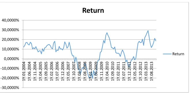
FIGURE 3 – Minimum variance portfolio returns, 1 year “data window”
FIGURE 4 – Minimum variance portfolio Sharpe Index, 1 year “data window”
-30,0000% -20,0000% -10,0000% 0,0000% 10,0000% 20,0000% 30,0000% 40,0000% 1Y .01.2 004 1Y .06.2 004 1Y .11.2 004 1Y .04.2 005 1Y .09.2 005 1Y .02.2 006 1Y .07.2 006 1Y .12.2 006 1Y .05.2 007 1Y .10.2 007 1Y .03.2 008 1Y .08.2 008 1Y .01 .2 00 9 1Y .06.2 009 1Y .11.2 009 1Y .04.2 010 1Y .09 .2 01 0 1Y .02.2 011 1Y .07.2 011 1Y .12.2 011 1Y .05 .2 01 2 1Y .10.2 012 1Y .03.2 013 1Y .08.2 013
Return
Return -2,0000 -1,0000 0,0000 1,0000 2,0000 3,0000 4,0000 1Y .01.2 004 1Y .06.2 004 1Y .11.2 004 1Y .04.2 005 1Y .09.2 005 1Y .02 .2 00 6 1Y .07.2 006 1Y .12.2 006 1Y .05.2 007 1Y .10.2 007 1Y .03.2 008 1Y .08.2 008 1Y .01 .2 00 9 1Y .06.2 009 1Y .11.2 009 1Y .04.2 010 1Y .09.2 010 1Y .02.2 011 1Y .07.2 011 1Y .12 .2 01 1 1Y .05.2 012 1Y .10.2 012 1Y .03.2 013 1Y .08.2 013Sharpe Index
Sharpe Index37
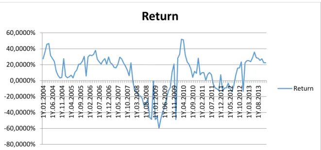
FIGURE 5 – Naïve portfolio returns, 1 year “data window”
FIGURE 6 – Naïve portfolio Sharpe Index, 1 year “data window”
-80,0000% -60,0000% -40,0000% -20,0000% 0,0000% 20,0000% 40,0000% 60,0000% 1Y .01.2 004 1Y .06.2 004 1Y .11.2 004 1Y .04.2 005 1Y .09.2 005 1Y .02.2 006 1Y .07.2 006 1Y .12.2 006 1Y .05.2 007 1Y .10.2 007 1Y .03.2 008 1Y .08.2 008 1Y .01 .2 00 9 1Y .06.2 009 1Y .11.2 009 1Y .04.2 010 1Y .09 .2 01 0 1Y .02.2 011 1Y .07.2 011 1Y .12.2 011 1Y .05 .2 01 2 1Y .10.2 012 1Y .03.2 013 1Y .08.2 013
Return
Return -2,0000 -1,0000 0,0000 1,0000 2,0000 3,0000 4,0000 1Y .01.2 004 1Y .06.2 004 1Y .11.2 004 1Y .04.2 005 1Y .09.2 005 1Y .02 .2 00 6 1Y .07.2 006 1Y .12.2 006 1Y .05.2 007 1Y .10.2 007 1Y .03.2 008 1Y .08.2 008 1Y .01 .2 00 9 1Y .06.2 009 1Y .11.2 009 1Y .04.2 010 1Y .09.2 010 1Y .02.2 011 1Y .07.2 011 1Y .12 .2 01 1 1Y .05.2 012 1Y .10.2 012 1Y .03.2 013 1Y .08.2 013Sharpe Index
Sharpe Index38
FIGURE 7 – Returns comparison of both 3 portfolios, 1 year “data window”
FIGURE 8 – Sharpe Index comparison of both 3 portfolios, 1 year “data window”
-100,0000% -50,0000% 0,0000% 50,0000% 100,0000% 150,0000% 1Y .01.2004 1Y .05.2004 1Y .09.2004 1Y .01.2005 1Y .05.2005 1Y .09.2005 1Y .01.2006 1Y .05.2006 1Y .09.2006 1Y .01.2007 1Y .05.2007 1Y .09.2007 1Y .01.2008 1Y .05 .200 8 1Y .09.2008 1Y .01.2009 1Y .05.2009 1Y .09.2009 1Y .01.2010 1Y .05.2010 1Y .09.2010 1Y .01.2011 1Y .05.2011 1Y .09.2011 1Y .01 .201 2 1Y .05.2012 1Y .09.2012 1Y .01.2013 1Y .05.2013 1Y .09.2013
Markowitz Return Minimum Variance Return Naïve Return
-2,0000 -1,0000 0,0000 1,0000 2,0000 3,0000 4,0000 1Y .01.2004 1Y .05.2004 1Y .09.2004 1Y .01.2005 1Y .05.2005 1Y .09.2005 1Y .01 .200 6 1Y .05.2006 1Y .09.2006 1Y .01 .200 7 1Y .05.2007 1Y .09.2007 1Y .01 .200 8 1Y .05.2008 1Y .09.2008 1Y .01 .200 9 1Y .05.2009 1Y .09.2009 1Y .01.2010 1Y .05.2010 1Y .09.2010 1Y .01.2011 1Y .05.2011 1Y .09.2011 1Y .01.2012 1Y .05.2012 1Y .09.2012 1Y .01.2013 1Y .05.2013 1Y .09.2013
39
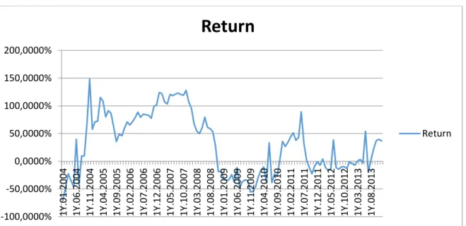
FIGURE 9 – Markowitz portfolio returns, 2 years “data window”
FIGURE 10 – Markowitz portfolio Sharpe Index, 2 years “data window”
-100,0000% -50,0000% 0,0000% 50,0000% 100,0000% 150,0000% 200,0000% 1Y .01.2 004 1Y .06.2 004 1Y .11.2 004 1Y .04.2 005 1Y .09.2 005 1Y .02.2 006 1Y .07.2 006 1Y .12.2 006 1Y .05.2 007 1Y .10.2 007 1Y .03.2 008 1Y .08.2 008 1Y .01.2 009 1Y .06.2 009 1Y .11.2 009 1Y .04.2 010 1Y .09.2 010 1Y .02 .2 01 1 1Y .07.2 011 1Y .12.2 011 1Y .05.2 012 1Y .10.2 012 1Y .03.2 013 1Y .08.2 013
Return
Return -1,0000 0,0000 1,0000 2,0000 3,0000 4,0000 1Y .01.2 … 1Y .08.2 … 1Y .03 .2 … 1Y .10.2 … 1Y .05.2 … 1Y .12.2 … 1Y .07.2 … 1Y .02.2 … 1Y .09.2 … 1Y .04.2 … 1Y .11.2 … 1Y .06.2 … 1Y .01.2 … 1Y .08.2 … 1Y .03.2 … 1Y .10.2 … 1Y .05.2 … 1Y .12.2 …Sharpe Index
Sharpe Index40
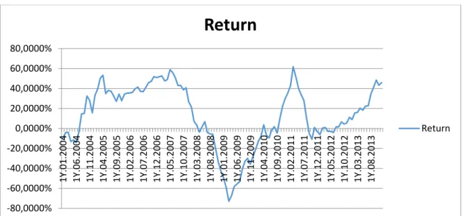
FIGURE 11 - Minimum variance portfolio returns, 2 years “data window”
FIGURE 12 – Minimum variance portfolio Sharpe Index, 2 years “data window”
-30,0000% -20,0000% -10,0000% 0,0000% 10,0000% 20,0000% 30,0000% 40,0000% 50,0000% 1Y .01.2 004 1Y .06.2 004 1Y .11.2 004 1Y .04.2 005 1Y .09.2 005 1Y .02.2 006 1Y .07.2 006 1Y .12.2 006 1Y .05.2 007 1Y .10.2 007 1Y .03.2 008 1Y .08.2 008 1Y .01 .2 00 9 1Y .06.2 009 1Y .11.2 009 1Y .04.2 010 1Y .09 .2 01 0 1Y .02.2 011 1Y .07.2 011 1Y .12.2 011 1Y .05 .2 01 2 1Y .10.2 012 1Y .03.2 013 1Y .08.2 013
Return
Return -1,50000 -1,00000 -0,50000 0,00000 0,50000 1,00000 1,50000 2,00000 2,50000 3,00000 1Y .01.2 004 1Y .07.2 004 1Y .01.2 005 1Y .07.2 005 1Y .01.2 006 1Y .07.2 006 1Y .01 .2 00 7 1Y .07.2 007 1Y .01.2 008 1Y .07.2 008 1Y .01.2 009 1Y .07.2 009 1Y .01.2 010 1Y .07.2 010 1Y .01.2 011 1Y .07.2 011 1Y .01.2 012 1Y .07.2 012 1Y .01.2 013 1Y .07 .2 01 3Sharpe Index
Sharpe Index41
FIGURE 13 – Naïve portfolio returns, 2 years “data window”
FIGURE 14 – Naïve portfolio Sharpe Index, 2 years “data window”
-80,0000% -60,0000% -40,0000% -20,0000% 0,0000% 20,0000% 40,0000% 60,0000% 80,0000% 1Y .01.2 004 1Y .06.2 004 1Y .11.2 004 1Y .04.2 005 1Y .09.2 005 1Y .02.2 006 1Y .07.2 006 1Y .12.2 006 1Y .05.2 007 1Y .10.2 007 1Y .03.2 008 1Y .08.2 008 1Y .01 .2 00 9 1Y .06.2 009 1Y .11.2 009 1Y .04.2 010 1Y .09 .2 01 0 1Y .02.2 011 1Y .07.2 011 1Y .12.2 011 1Y .05 .2 01 2 1Y .10.2 012 1Y .03.2 013 1Y .08.2 013
Return
Return -2,0000 -1,0000 0,0000 1,0000 2,0000 3,0000 4,0000 1Y .01.2 004 1Y .06.2 004 1Y .11.2 004 1Y .04.2 005 1Y .09.2 005 1Y .02 .2 00 6 1Y .07.2 006 1Y .12.2 006 1Y .05.2 007 1Y .10.2 007 1Y .03.2 008 1Y .08.2 008 1Y .01 .2 00 9 1Y .06.2 009 1Y .11.2 009 1Y .04.2 010 1Y .09.2 010 1Y .02.2 011 1Y .07.2 011 1Y .12 .2 01 1 1Y .05.2 012 1Y .10.2 012 1Y .03.2 013 1Y .08.2 013Sharpe Index
Sharpe Index42
FIGURE 15 – Returns comparison of both 3 portfolios, 2 years “data window”
FIGURE 16 – Sharpe Index comparison of both 3 portfolios, 2 years “data window”
-100,0000% -50,0000% 0,0000% 50,0000% 100,0000% 150,0000% 200,0000% 1Y .01.2004 1Y .05.2004 1Y .09.2004 1Y .01.2005 1Y .05.2005 1Y .09.2005 1Y .01.2006 1Y .05.2006 1Y .09.2006 1Y .01.2007 1Y .05.2007 1Y .09.2007 1Y .01.2008 1Y .05 .200 8 1Y .09.2008 1Y .01.2009 1Y .05.2009 1Y .09.2009 1Y .01.2010 1Y .05.2010 1Y .09.2010 1Y .01.2011 1Y .05.2011 1Y .09.2011 1Y .01 .201 2 1Y .05.2012 1Y .09.2012 1Y .01.2013 1Y .05.2013 1Y .09.2013
Markowitz Return Minimum Variance Return Naïve Return
-2,0000 -1,0000 0,0000 1,0000 2,0000 3,0000 4,0000 1Y .01.2004 1Y .05.2004 1Y .09.2004 1Y .01.2005 1Y .05.2005 1Y .09.2005 1Y .01 .200 6 1Y .05.2006 1Y .09.2006 1Y .01 .200 7 1Y .05.2007 1Y .09.2007 1Y .01 .200 8 1Y .05.2008 1Y .09.2008 1Y .01 .200 9 1Y .05.2009 1Y .09.2009 1Y .01.2010 1Y .05.2010 1Y .09.2010 1Y .01.2011 1Y .05.2011 1Y .09.2011 1Y .01.2012 1Y .05.2012 1Y .09.2012 1Y .01.2013 1Y .05.2013 1Y .09.2013