Conservation planning of threatened flora in northwest Iberian Peninsula: a comparison of two reserve selection tools

(1)

Conservation

planning of

threatened flora in

northwest Iberian

Peninsula: a

comparison of two

reserve selection

tools

Ricardo Reis Alves Soares Cardoso

Dissertação de Mestrado apresentada à

Faculdade de Ciências da Universidade do Porto em 13/12/2013

Ciências e Tecnologia do Ambiente

2013

Rica rd o Reis A lv es S o ar es Car d o so FCUP 2013 2.º CICLO

(2)

planning of

threatened flora in

northwest Iberian

Peninsula: a

comparison of two

reserve selection

tools

Ricardo Reis Alves Soares Cardoso

Mestrado em Ciências e Tecnologias do Ambiente

Departamento de Geociências, Ambiente e Ordenamento do Território 2013

Orientador

Prof. Dr. João José Pradinho Honrado, Professor Auxiliar, FCUP

Coorientador

Doutora Ângela Cristina de Araújo Rodrigues Lomba, Investigadora Pós-Doutoral, FCUP

(3)

(4)

(5)

(6)

Resumo

O planeamento sistemático da conservação é um conjunto de etapas utilizadas para a identificação eficiente de áreas e implementação de ações de conservação que garantam a representação e a persistência das espécies. Uma importante etapa do planeamento sistemático para a conservação consiste na seleção de novas áreas de conservação, quer como novas redes de reservas, quer para complementar redes de áreas de conservação já existentes. A seleção de reservas é geralmente feita com recurso algoritmos de seleção de reservas. Nesta dissertação, apresentam-se os dois principais tipos de problemas de seleção de reservas e faz-se uma revisão dos vários tipos de algoritmos existentes para os resolver, nomeadamente algoritmos heurísticos, metaheurísticos e exatos. Em seguida, são descritos em detalhes dois programas de

planeamento de conservação – Marxan e ConsNet. Ambas as ferramentas

implementam algoritmos metaheurísticos: simulated annealing no caso do Marxan, e tabu search no ConsNet. Investigou-se a performance relativa destes programas no problema de encontrar o menor conjunto de locais garantindo que os elementos de conservação atinjam metas de representação predefinidas. Para tal, usaram-se as distribuições observadas e as previstas de 11 espécies de plantas raras ou ameaçadas na Galiza e Norte de Portugal. Compararam-se os atributos espaciais e a sobreposição das soluções. Os resultados mostram que o ConsNet produziu redes de conservação com menor área, enquanto o Marxan produziu soluções mais compactas. Ambos os programas selecionaram locais nas mesmas áreas geográficas, embora as células selecionadas não tenham tido uma elevada sobreposição. Com base nestes resultados, sugere-se o uso do ConsNet quando o objetivo é encontrar a menor área, e o Marxan quando uma solução mais compacta é mais importante que uma de menor custo.

Palavras-chave: Algoritmos de seleção de reservas; ConsNet; Galiza; Marxan; Norte de Portugal; Planeamento sistemático da conservação; Simulated annealing; Tabu search

(7)

Abstract

Systematic conservation planning is a framework developed to efficiently identify conservation areas and implement conservation actions that guarantee species representation and persistence. An important stage of systematic conservation planning is the selection of new conservation areas, either as a new reserve network or to complement existing conservation area networks. Reserve selection is often done with the support of computer algorithms. In this dissertation, the two main types of reserve selection problems are presented and various types of reserve selection algorithms are reviewed, specifically heuristics, metaheuristics and optimal algorithms. Then, Marxan and ConsNet, two conservation planning software packages are described in detail. Both tools implement metaheuristic algorithms: simulated annealing in the case of Marxan, and tabu search in ConsNet. We investigated the relative performance of these programmes in finding the smallest set of sites such that conservation features meet predefined targets. To do this, we used data on the observed and predicted distributions of 11 rare or threatened plant species in Galicia and Northern Portugal. We compared the spatial attributes of the solutions and their overlap. Results show ConsNet produced smaller reserve networks, while Marxan generated more compact solutions. The same broad geographic regions were selected by both packages for expansion of the existing protected areas, although the specific cells selected did not show a high overlap. Based on these results, we suggest using ConsNet when attempting to find the smallest area, and Marxan when compactness is more important than minimizing the cost.

Keywords: ConsNet; Galicia; Marxan; Northern Portugal; Reserve selection algorithms; Simulated annealing; Systematic conservation planning; Tabu search

(8)

Acknowledgments

This research was developed at FCUP within project “Biodiversidad Vegetal

Amenazada Galicia-Norte de Portugal. Conocer, gestionar e implicar”

(0479_BIODIV_GNP_1_E), funded by "2º Eixo prioritário – Cooperação e Gestão

Conjunta e Meio Ambiente, Património e Gestão de Riscos" of the "Programa

Operacional de Cooperação Transfronteiriça Espanha – Portugal (POCTEP) 2007-

2013".

I would like to thank my supervisor, Professor João Honrado, and co-supervisor, Dr. Ângela Lomba, for giving me the opportunity to work on this exciting subject, as well as for their guidance and support.

I am thankful to Rui Fernandes, for all of his assistance in creating the input files and using GIS software.

I extend my deepest gratitude to my family, for their words of encouragement and for supporting me in this journey.

Finally, I am deeply thankful to my girlfriend, Carla, for her unwavering support, encouragement, patience and love. The successful completion of this work was only possible because of her words and actions.

(9)

List of Figures

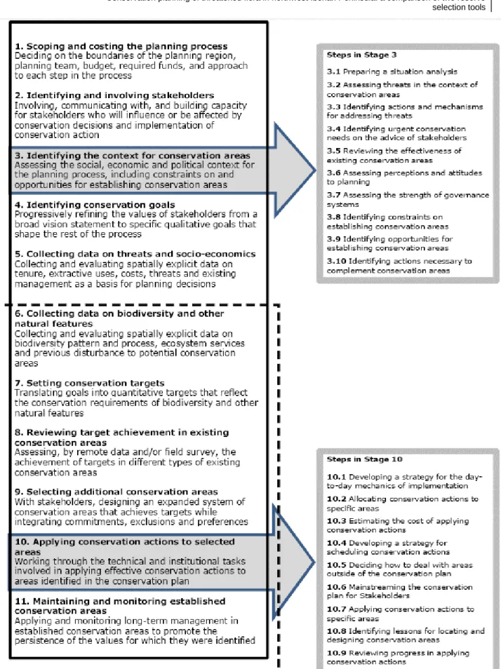
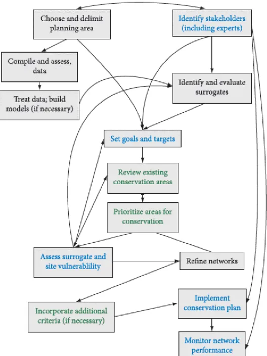
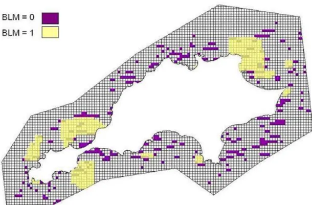
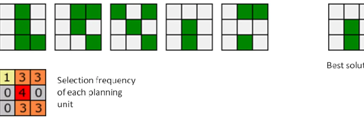
Figure 1. An evolving framework for conservation planning with 11 main stages. Text under the heading for each stage summarizes the main issues to be addressed (see Margules & Pressey 2000; Cowling & Pressey 2003 for more detail on most stages). For convenience, the process is depicted as a linear sequence, but in reality some stages will be undertaken simultaneously and there are many feedbacks from later to earlier stages. Among the reasons for feedbacks are revisions of earlier steps to deal with surprises, including unexpected opportunities. The dashed rectangle contains the stages described by Margules and Pressey (2000). The steps involved in stages 3 and 10 are included to emphasize the diversity of tasks and decisions involved. Source: Pressey and Bottrill (2008). ... 5 Figure 2. Stages of Systematic Conservation Planning. Arrows indicate which components directly influence which others. A bidirectional arrow indicates feedback. Only the major interactions between the components are shown. There is potential for feedback between almost any two components of this framework. Boxes with text in green indicate aspects that are well-understood, those with text in black are aspects which are fairly well-understood, and those with blue text are areas that remain poorly understood and subject to much ongoing research. Source: Sarkar and Illoldi-Rangel (2010). ... 6 Figure 3. Effect of BLM on the spatial configuration of the reserve network. A BLM of 0 results in a highly fragmented solution (in purple), albeit with smaller total area. A BLM of 1 produces a much more compact solution (in yellow), at the expense of a larger total area. ... 18 Figure 4. Example outputs from 5 runs of Marxan on a dataset with 9 cells. The first five grids represent the solution for each run. The grid labelled “Best solution” corresponds to the solution with the fewest cells. The bottom grid displays the selection frequency of each cell, i.e. the number of times each cell was selected across the 5 runs. The higher this value, the more important that cell is for achieving the representation targets efficiently. ... 23 Figure 5. Screenshot of the Zonae Cogito graphing functionality. Here a tradeoff curve has been plotted between boundary length and cost, a common approach to calibrating the BLM parameter in Marxan. ... 25

(12)

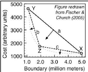
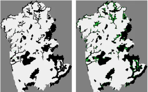
Figure 6. Available trade-off between minimizing cost and minimizing boundary length. Dotted gray line represents possible solutions on the trade-off curve. Solution X is the lowest cost solution available. Solution Y has the smallest boundary length. Solution Z achieves large reductions in boundary length for a small increase in cost (compared to X). The dashed lines “b” and “c” represent the estimated trade-off curve with three solutions “X”, “Y” and “Z”. Source: Ardron et al. (2010). ... 37 Figure 7. ConsNet (left) and Marxan (right) solutions for scenario A1. The existing reserve network is in black, while the additional area selected by the algorithms is in green. ... 43 Figure 8. ConsNet (left) and Marxan (right) solutions for scenario A2. The existing reserve network is in black, while the additional area selected by the algorithms is in green. ... 43 Figure 9. ConsNet (left) and Marxan (right) solutions for scenario A3. The existing reserve network is in black, while the additional area selected by the algorithms is in green. ... 43 Figure 10. ConsNet (left) and Marxan (right) solutions for scenario B1. The existing reserve network is in black, while the additional area selected by the algorithms is in green. ... 44 Figure 11. ConsNet (left) and Marxan (right) solutions for scenario B2. The existing reserve network is in black, while the additional area selected by the algorithms is in green. ... 44 Figure 12. ConsNet (left) and Marxan (right) solutions for scenario B3. The existing reserve network is in black, while the additional area selected by the algorithms is in green. ... 44

(13)

List of Tables

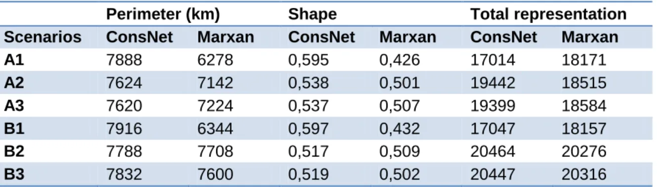
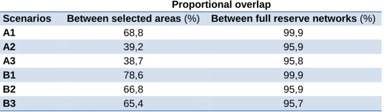
Table 1. Plant species used in the analysis, their conservation status and their observed and predicted occurrences. ... 33 Table 2. Total area, number of clusters and average area of clusters identified by ConsNet and Marxan, for each scenario. ... 40 Table 3. Perimeter, shape (perimeter-to-area ratio) and total representation of solutions produced by ConsNet and Marxan, for each scenario. ... 40 Table 4. Proportional overlap between solutions produced by Marxan and ConsNet. “Selected areas” refers to the areas added to the existing reserve network. “Full reserve networks” are the solutions as reported by the programs, i.e. including the existing protected area network. ... 42

(14)

List of Abbreviations

BLM – Boundary Length Modifier

CLUZ – Conservation Land-Use Zoning software CR – Critically Endangered

DNS – Dynamic Neighbourhood Selection EN – Endangered

GIS – Geographic Information System GUI – Graphical User Interface

ID – Identification

IUCN – International Union for Conservation of Nature MASTS – Modular Adaptive Tabu Search

NP – Non-Deterministic Polynomial Time PA – Protected Areas

PANDA – Protected Areas Network Design Application RBO – Rule-Based Objective

SDM – Species Distribution Models SLOSS – Single Large or Several Small SPF – Species Penalty Factor

UTM – Universal Transverse Mercator US – United States of America

(15)

Chapter 1. Introduction and objectives

1.1. The decline of biodiversity and the role of protected areas

Biodiversity can be defined as the variation among living organisms, including diversity and interaction within species, between species and of ecosystems (Carvalho, 2010; United Nations Environment Programme, 1992). Biodiversity plays a key role in ecosystem functioning and the provision of ecosystem services (Millennium Ecosystem Assessment, 2005). A recent review found a large number of ecosystem services benefit from an increase in biodiversity, some suffer mixed effects and a small number are hindered by higher biodiversity (Cardinale et al., 2012).

In spite of its significance, biodiversity is declining at an alarming rate, only comparable to the last mass extinction (Koh et al., 2004; Pimm et al., 1995; Wake and Vredenburg, 2008). This loss of biodiversity has led to the degradation of an estimated 60% of Earth’s ecosystem services over the last 50 years(Millennium Ecosystem Assessment, 2005). The major drivers of this decline include overexploitation of biological resources, habitat conversion and fragmentation, climate change, proliferation of invasive species, pollution and genetic depletion (Davies et al., 2006; Ehrlich and Pringle, 2008; Parmesan, 2006; Thomas et al., 2004).

One of the approaches to address this biodiversity decline is through in situ protection, namely with the designation of protected areas (Margules and Pressey, 2000; Primack, 2006). Protected areas are one of the most effective methods for the protection and conservation of biodiversity (Rodrigues et al., 2004), and the global coverage of protected areas has steadily increased in the last decades (Mulongoy and Chape, 2004). In 2004, Rodrigues et al. assessed the global protected areas network for its coverage of the distribution of 11,633 terrestrial vertebrates, and observed that 1,424 (12%) species were not represented in any of the protected areas. Moreover, outcomes for Rodrigues et al. assessment highlighted an underrepresentation of threatened species, and from such species, 20% were identified as gap species.

1.2. Systematic Conservation Planning

Conservation planning is the process of locating, configuring, implementing and maintaining areas that are managed to promote the persistence of biodiversity and other natural values (Pressey et al., 2007). In conservation planning, species richness,

(16)

rarity, level of endemism or threat or other geographic, social or economic indices are used to prioritize areas to conserve (Carvalho, 2010). Global key areas for conservation have been identified by several biodiversity conservation organizations using these strategies (Brooks et al., 2006). In order to establish explicit conservation goals that can be translated into quantitative targets towards which progress can be measured, a new framework has been developed called systematic conservation planning (Margules and Pressey, 2000; Pressey and Bottrill, 2008; Sarkar and Illoldi-Rangel, 2010).

Systematic conservation planning is a framework developed to efficiently identify conservation areas that guarantee species representation and persistence (Margules and Pressey, 2000; Moilanen et al., 2009) Representation refers to the need to represent all features of biodiversity, preferably at all levels of organization. Persistence refers to long-term survival of the species and other features of biodiversity, achieved by maintaining the ecological and evolutionary processes that sustain them (Carvalho, 2010; Margules and Pressey, 2000). Both of these goals should be achieved with as much economy of resources as possible, because resources for biodiversity conservation are limited and their allocation should be optimized. Additionally, considering such resources could potentially be used to promote human well-being, their efficient allocation is an ethical imperative (Sarkar and Illoldi-Rangel, 2010). Systematic conservation planning has a number of distinctive features, such as assessing the achievement of conservation goals in existing reserves prior to the planning process and the use of explicit methods to locate and design new reserves (Margules and Pressey, 2000). Additionally, it is guided by the following set of key principles (Carvalho, 2010; Wilson et al., 2009a):

 Comprehensiveness and representativeness: a comprehensive conservation

network includes a fraction of each element of biodiversity; while a representative conservation network assures that each biodiversity element is sufficiently represented, for example by including viable populations.

 Complementarity and efficiency: efficiency refers to the need to achieve

conservation goals at the lowest possible cost. Complementarity ensures that the different areas of a conservation network complement each other in terms of the type and amount of biodiversity elements they contain. It is a measure of the extent to which an area contributes unrepresented features to an existing area or set of areas (Margules and Pressey, 2000).

(17)

 Flexibility and irreplaceability: flexibility can be defined as the number of possible combinations of sites that can be selected to attain the representation targets efficiently. Irreplaceability, on the other hand, is a measure of how indispensable a site is for meeting the representation targets. An irreplaceable site is one without which one or more targets will not be met (Carwardine et al., 2006).

 Adequacy: this principle ensures a conservation network promotes the

persistence and evolution of the biodiversity elements represented. The lack of data or limited understanding of the ecological and evolutionary processes that sustain species persistence mean this principle is commonly neglected. It has been addressed by setting targets based on population viability analyses or probabilities of persistence, including spatial configuration criteria such as reserve size, connectivity and shape and identifying surrogates for ecological and evolutionary processes (Carvalho, 2010).

Margules and Pressey (2000) originally described six stages in the process of systematic conservation planning. Pressey and Bottrill (2008) describe 5 additional

stages. Their proposed framework is depicted in Erro! Auto-referência de marcador

inválida.. Sarkar and Illoldi-Rangel (2010) offer another protocol for systematic conservation planning, which is not as detailed in the early stages but has additional steps at the final stages (Figure 2) This protocol also makes explicit the main interactions between the stages and the degree to which they are well understood. It is important to note that, more than being a theoretical framework, systematic conservation planning is already being considered in the decisions of organizations, influencing legislation and policy and accomplishing results on the ground and in the water (Pressey and Bottrill, 2008).

(18)

1.3. Objectives

This dissertation has three main objectives:

1. To review the concepts and technical choices that underlie the development of conservation planning software tools.

2. To describe two spatial conservation prioritization software tools: ConsNet (Ciarleglio et al., 2009) and Marxan (Ball et al., 2009).

3. To compare the performance of ConsNet and Marxan, using a subset of the dataset from BIODIV_GNP “Threatened Biodiversity – Galicia and Northern Portugal” project, in order to test distinct tools for their adequacy in the establishment of complementary areas of protection for threatened plant species.

(19)

Figure 1. An evolving framework for conservation planning with 11 main stages. Text under the heading for each stage summarizes the

main issues to be addressed (see Margules & Pressey 2000; Cowling & Pressey 2003 for more detail on most stages). For convenience, the process is depicted as a linear sequence, but in reality some stages will be undertaken simultaneously and there are many feedbacks from later to earlier stages. Among the reasons for feedbacks are revisions of earlier steps to deal with surprises, including unexpected opportunities. The dashed rectangle contains the stages described by Margules and Pressey (2000). The steps involved in stages 3 and 10 are included to emphasize the diversity of tasks and decisions involved. Source: Pressey and Bottrill (2008).

(20)

Figure 2. Stages of Systematic Conservation Planning. Arrows indicate which components directly influence which

others. A bidirectional arrow indicates feedback. Only the major interactions between the components are shown. There is potential for feedback between almost any two components of this framework. Boxes with text in green indicate aspects that are well-understood, those with text in black are aspects which are fairly well-understood, and those with blue text are areas that remain poorly understood and subject to much ongoing research. Source: Sarkar and Illoldi-Rangel (2010).

(21)

Chapter 2. Reserve selection tools

2.1. Introduction

Early efforts at reserve design were guided by the equilibrium theory of island biogeography and related biogeographical theory (Margules and Pressey, 2000; Possingham et al., 2000; Sarkar et al., 2006). Emphasis was on the size, shape and number of reserves. This body of theory prescribes general guidelines about the preferable way to design a reserve network. For instance: bigger reserves are better than small reserves; long and thin reserves with a high edge-to-area ratio are worse than compact, circular ones; reserves should be connected by habitat corridors instead of isolated from each other, and so on (Margules and Pressey, 2000; Possingham et al., 2000). An early debate, known in the scientific literature as the SLOSS debate (single large or several small), occurred over whether species richness is maximized in one large reserve or in several smaller ones of equal total area (Primack, 2006). The proponents of large parks argued that only large reserves had sufficient numbers of large, wide-ranging, low-density species (such as large carnivores) to assure the persistence of their populations. It was also argued that large reserves minimize the edge-to-area ratio, encompass more species, and can have greater habitat diversity than small reserves. Some evidence confirms some of these claims. In a study of mammal populations in 14 national parks of Western North America, local extinction rates were very low or zero in parks over 1000 km2 and much higher in parks smaller than that (Newmark, 1995). It is also true that human population densities are lower on the edge of large reserves compared with those on the edge of small reserves. This could contribute to the higher extinction rates in small parks (Parks and Harcourt, 2002; Wiersma et al., 2004).

On the other hand, once a park reaches a certain size, the number of new species added with each increase starts to decline. At that point, creating a second large park, as well as a third or fourth park some distance away, may be an effective strategy for conserving additional species (Primack, 2006). Some proponents of large reserves argued that small reserves need not be maintained, because their inability to support long-term population, ecosystem processes and all stages of ecological succession gave them little value for conservation purposes. Other conservation biologists argued that well-placed small reserves are able to include a greater diversity of habitat types and more populations of rare species than one large block of equivalent area (Shafer,

(22)

1995; Simberloff and Gotelli, 1984). Small reserves are particularly important for the protection of many species of plants, invertebrates and small vertebrates (Schwartz, 1999). The value of several well-placed reserves in different habitats was demonstrated by a comparison of four national parks in the United States (Primack, 2006). The total number of large mammalian species in three parks located in contrasting habitats is greater than the number of species in the largest US park, Yellowstone, even though the area of Yellowstone is larger than the combined area of the other three parks. Creating more reserves, even small ones, decreases the chance

of a single catastrophic event – such as an invasive species, a disease or fire –

destroying an entire species (Primack, 2006).

It has been argued the debate was a product of the island-biogeographic foundation of reserve design theory and ended in the inconclusive answer “it depends” (Possingham et al., 2000). Importantly, the island biogeography approach makes the assumption, which is often invalid, that reserves are habitat islands completely isolated by an unprotected matrix of inhospitable terrain. In fact, many species are capable of living in and dispersing through this habitat matrix (Primack, 2006).

Despite giving some insights into reserve design, the guidelines provided by island bio-geography offer little explicit guidance for decision-makers who are faced with specific choices about how many, which sites or which spatial configuration to include in a reserve network. For these reasons, reserve selection shifted its focus to systematic conservation planning, with its emphasis on quantitative targets, representativeness and efficiency (Margules and Pressey, 2000). The quantitative targets for species (or any other biodiversity feature) representation are often called representation targets. These can be the number of occurrences of a feature (e.g. a species) required in a reserve or the fraction of its total area of occurrence (e.g. a vegetation type) that must be included.

2.2. Formalization of conservation problems

In order to properly design and implement software planning tools, it is important to precisely specify both the problems to be solved and the algorithms to solve them. The formal problems relevant to reserve selection have been studied for a long time within computer science and operations research (Cerdeira and Pinto, 2005; Daskin, 1983; Hoffman and Padberg, 2001; Krarup and Pruzan, 1983; Paschos, 1997).

(23)

2.2.1. Constrained optimization

Problems solved by reserve selection tools can usually be formalized as constrained optimization (maximization or minimization) problems (Sarkar et al., 2006). One standard problem is to find the smallest set of sites such that all the representation targets are met. The quantity being optimized (minimized) is the number of sites; the constraint is that all the targets must be met. Formulating problems as constrained optimization problems is useful because a range of algorithms with known performance are available for solving them.

2.2.2. Reserve network selection problems

Numerous optimization problems can be formulated as mathematical programming problems (Cocks and Baird, 1989). A family of problems that occur in the design of reserve networks are variants of the “set cover” (also known as minimum set) and “maximal cover” (also known as maximum coverage) problems studied in operations research (Camm et al., 2002; Church et al., 1996; Possingham et al., 2000; ReVelle et al., 2002; Sarkar et al., 2006). The basic inputs of these problems are a set of sites constituting a planning region and a list of the conservation features occurring in each site. In the set cover problem, the goal is to minimize the total cost of the selected sites, while meeting a set of representation targets for the features. In a more formal formulation, let m be the total number of sites and n the number of different

conservation features (e.g. species, vegetation types). Each site has a cost and

each feature has a target . The variable equals 1 if site is selected, otherwise it

equals 0. The contribution to the conservation of feature by the selection of site is

contained in a matrix with elements . The objective is to minimize the cost:

∑

subject to the constraint that the representation targets are met:

∑

The “set cover” problem may assume simple or complex forms. Every site might be assumed to have the same cost, in which case the objective is to minimize the number of sites selected, or the cost can reflect actual monetary, management and/or opportunity costs. Each feature may be described in similar or different units (e.g.,

(24)

number of individuals, extent of occurrence, probability of occurrence) and individual targets can be set for each feature (Wilson et al., 2009b).

In the “maximal cover” problem, the objective is to maximize some measure of benefit, subject to a limit on the resources that can be expended (Wilson et al., 2009b). In a simple case, the measure of benefit might be the number of features that meet their targets, and the limit may be set for the number of sites that can be selected. Formally, the objective is to maximize

∑ ( ( ))

subject to

∑

where and are as previously defined, and is the amount of feature conserved

in reserve system , and is a function that turns that into a value. The maximum

available budget is , which is in the same units as . As in the set cover problem,

there are multiple versions of the maximal cover problem. The “maximal cover”

problem can be solved without using targets and the budget may or may not be sufficient for meeting all targets and may be updated through time if more or fewer funds become available. In the simplest case, if the target for feature is achieved, equals 1, otherwise it equals 0. Alternatively, the benefit can be measured by a set of functions representing the incremental gains in the conservation of each feature per dollar invested. These functions can be linear, meaning the benefits are proportional to the amount invested, or curved, to represent situations where there are diminishing or increasing benefits for each dollar invested. Features may be differentially weighted to emphasize investment in those that are of higher conservation concern, such as rare, endemic or threatened species (Arponen et al., 2007).

The basic versions of both problems can be represented as deterministic integer programming problems (Sarkar et al., 2004). Other goals can be incorporated as further constraints, such as shape (perimeter-to-area ratio) or the minimum size of clusters (contiguous sets of selected sites) (ReVelle et al., 2002; Rodrigues et al., 2000).

(25)

2.2.3. Multicriteria analysis

The allocation of land for biodiversity conservation frequently competes with alternative uses, such as agriculture, forestry, extractive activities, urbanization and recreation. Ignoring these alternative claims on land results in political problems and possible failure of conservation plans (Pierce et al., 2005; Sarkar et al., 2006). Therefore, effective conservation planning must take political and socioeconomic factors into account (Possingham & Stewart 2005; Knight et al. 2006; Lagabrielle et al. 2010). These can be integrated into reserve selection by using multicriteria analysis. Multicriteria analysis also allows for the incorporation of criteria relevant to the spatial configuration of the reserve networks, such as size, shape, replication, connectivity and dispersion, which play a determining role in the persistence of biodiversity (Margules and Pressey, 2000).

There are two types of protocols for incorporating multiple criteria into reserve selection, referred to as iterative stage protocols and terminal stage protocols (Sarkar et al., 2006). In iterative stage protocols, multiple criteria are considered as each site (or small set of sites) is selected for inclusion. One notable example is Marxan (Ball et al., 2009), which incorporates relevant criteria in its objective function. In the second type, terminal stage protocols, sets of potential reserve networks are identified on the basis of a given criterion, usually biodiversity representation, and further socioeconomic criteria are then used to select one of the potential reserves. ConsNet (Ciarleglio et al., 2009) is an example of a conservation planning tool that employs a terminal stage protocol. Both types can be used simultaneously, with some criteria incorporated during site selection and some at the end. Moffett and Sarkar (2006) noted that existing planning tools only incorporate a small fraction of the techniques available for multicriteria analysis.

2.2.4. Probabilistic data

Traditionally, reserve selection algorithms were used with distributional data that showed whether a feature was present or absent and, occasionally, its abundance or extent. A common issue is that frequently the available information consists on presence-only, and not presence-absence data. One way to minimize the problems caused by presence-only data is to model the potential distribution of features (e.g., species) in the planning region (Elith et al., 2006; Guisan and Zimmermann, 2000). Species distribution models (SDM) seek to quantify the relationship between species

(26)

and their environment (Elith and Leathwick, 2009). They have been used to identify the main environmental variables that influence species’ distributions (Guisan and Thuiller, 2005) and to predict their potential distributions under current conditions and future environmental change (Thuiller, 2004).Typical outputs consist of probabilities of occurrence of species for each site (Cabeza et al., 2004; Elith and Leathwick, 2009; Guisan and Thuiller, 2005; Phillips and Dudík, 2008).

Probabilistic data can be converted into binary (presence-absence) data by using a threshold probability (Carvalho et al., 2010). However, this procedure has been criticized because the choice of the threshold is arbitrary (Sarkar et al., 2004). There are two different strategies to use probabilistic data directly (Sarkar et al., 2006). In the first strategy, occurrence probabilities in individual sites are compounded to obtain the corresponding probabilities for the entire region. The objective then is to ensure the probability in the reserve network is higher than a specified valued, similar to a representation target. Although frequently adopted, this strategy assumes the independence of the probabilities of different features in the same site and of the same feature in different sites. Due to the ecological relationships between features and to the spatial autocorrelation of their distributions (Koenig, 1999), these assumptions are unrealistic. In the second strategy, the probabilities are interpreted as expectations (or expected numbers of occurrences) of the conservation features in sites. The expected values of occurrences can be summed across the whole area without assumptions of independence (Sarkar et al., 2004). In this case, the goal is that the expected total number of occurrences has to be higher than a representation target, just like with binary data. Simultaneous use of both probabilistic and binary data doesn’t present a problem.

2.3. Algorithms and software

When designing algorithms to be incorporated in software tools, the main concern is with computational efficiency (or speed). For a better understanding of these issues, we introduce relevant terminology from computer science.

2.3.1. Computational complexity

Computational complexity is an attribute of a computational problem or algorithm and can be either a) temporal complexity, or the time required for a computation, with

(27)

complexity being the inverse of efficiency; or b) spatial complexity, or the amount of memory necessary for a computation (Sarkar et al., 2006).

Regarding temporal complexity, a computational problem is said to belong to class P (for polynomial time) if the number of elementary operations (additions, subtractions, multiplications and divisions) required to obtain an answer increases as a polynomial function of the size of the input (preferably a low-order polynomial). The important thing here is that such algorithms are tractable, i.e. the time required to execute them (a polynomial function) does not grow inordinately fast as the size of the problem increases, compared to an algorithm that grows at an exponential rate. Problems are said to belong to class NP (for non-deterministic polynomial time) if the number of operations required to verify a solution grows as a polynomial function of the size of the input (Cormen et al., 2001). The contrast here is between the time required to produce a solution (for P problems) and that required to verify if a solution is correct (in the case of NP). P is at least a subclass of NP. One of the most important open problems in computer science is whether P = NP.

Given these definitions, a problem is said to be NP-complete if a) it is in NP and b) every other problem in NP is reducible to it, i.e. any such problem can be transformed into the NP-complete problem using a P algorithm. NP-complete problems are the hardest problems in NP. Finally, an NP-hard problem is one that satisfies clause (b) above but not (a); that is, it isn’t necessarily in NP. Thus, NP-hard problems are at least as hard as complete problems, possibly harder. The most important aspect of NP-complete and NP-hard problems is that increasing the speed of computer processors does not significantly alter the tractability of these problems (Garey and Johnson, 1979). However, this doesn’t mean that every or even most instances of these problems cannot be solved efficiently. All it means is that there are instances for which a solution cannot be obtained in a reasonable amount of time, which represents an important restriction if the objective is to design generic software tools (Sarkar et al., 2006).

2.3.2. Heuristic algorithms

In reserve network design, both the set cover and maximal cover problems are NP-hard (Camm et al., 2002). Thus, exact or optimal algorithms, which are guaranteed to produce the optimal solutions (i.e. the most economical), may be intractable in many instances. However, for presence-absence data, the function to optimize can be

(28)

linearized, reducing temporal complexity. For probabilistic data, some problems can also be represented linearly (Camm et al., 2002; Sarkar et al., 2004). Nevertheless, because even the linearized problems are NP-hard, it is important to develop efficient heuristic algorithms (or heuristics).

A number of stepwise or “single pass” heuristics have been devised. A stepwise algorithm consists of a rule (or a series of rules), according to which potential sites are ranked and the highest-ranking site is selected. The remaining sites are ranked again and the process is repeated until termination. Despite being efficient due to the simplicity of the rules incorporated in them, most of these heuristics were developed with spatial economy and transparency in mind, the latter being achieved through the inclusion of biologically relevant criteria, such as complementarity, rarity and adjacency (Sarkar et al., 2006).

The heuristic rules most frequently used for the selection of reserves are a) to maximize complementarity of conservation features (“complementarity rule”) and b) to maximize rarity of the features in a site, with rarity defined as the inverse of the frequency or extent of occurrence of a feature (“rarity rule”). Multiple tests on a variety of artificial and empirical data have shown that, for binary data, using both rules produces the best results (Csuti et al., 1997; Sarkar et al., 2002). For probabilistic data, it is best to use the complementarity rule (Sarkar et al., 2004). This rule has been incorporated in various planning tools such as C-Plan (Pressey et al., 2009) and WorldMap (Vane-Wright et al., 1991; Williams, 2001). ResNet (Kelley et al., 2002; Sarkar et al., 2002) incorporates both rules.

Stepwise heuristic rules are implemented in a hierarchic fashion. In case one of the rules leads to a tie between two or more sites for inclusion, a second rule is used, and this process is repeated for the set of rules. For instance, if rarity causes a tie, an adjacency rule, which gives preference to sites adjacent to one already selected, can be used to try to break the tie. The use of an adjacency rule leads to the selection of larger clusters (Nicholls and Margules, 1993). In this way, hierarchical rules allow an intuitive incorporation of multiple criteria. However, the relative importance the rules is determined by their sequence, with frequency of rule use largely determined by the number of ties. This can lead to weightings of the rules that are not explicit (Sarkar et al., 2006).

A more recent and sophisticated use of heuristics can be found in the Zonation prioritization software (Moilanen, 2007; Moilanen et al., 2005). The Zonation algorithm

(29)

starts from the selection of the whole planning region, and iteratively removes the site that causes the smallest marginal loss of conservation value. Because Zonation does not aim to achieve specific representation targets, this process is repeated for every site, thus producing a hierarchy of conservation priorities for the entire landscape. The critical part of the algorithm is the definition of marginal loss (called the cell-removal rule), which also allows species weighting and species-specific connectivity considerations to be applied. Different cell-removal rules can be applied to emphasize different objectives, such as the retention of high-quality core areas for all species (Core-area Zonation), high average representation, at the cost of potential poor representation of some species (additive benefit function variant), or even target-based planning (through a special formulation of benefit functions) (Moilanen, 2007).

2.3.3. Metaheuristic algorithms

Before defining the term “metaheuristic”, it is useful to introduce some terminology from mathematical optimization. For constrained optimization problems, a feasible solution is any solution that satisfies all the constraints. The set of all feasible solutions for a problem is called the feasible region, or search space. A solution is called a local optimum if all neighbouring solutions are worse than it. It is analogous to a local maximum (minimum) of a function. The global optimum is the best solution from among all feasible solutions. In the set cover problem, it is the set of sites which satisfy the representation targets for the least possible cost. In the maximal cover problem it is the set of sites that satisfies targets for the highest number of features, subject to a given cost limit. The global optimum is analogous to a global maximum (minimum) of a function.

With these definitions in mind, we can define a metaheuristic algorithm (or simply metaheuristic) as an algorithm that repeatedly uses a set of heuristic rules to explore the search space and escape from local optima (Illoldi-Rangel et al., 2012). Contrary to exact algorithms, metaheuristics are not guaranteed to produce optimal solutions. However, they provide an efficient method for producing good or near-optimal solutions. Metaheuristic algorithms can be used to incorporate multiple criteria. For example, an initial selection of sites can be followed by repeated random substitution of sites to find out if a better spatial arrangement can be achieved without sacrificing representation targets (Sarkar et al., 2006). Termination of the algorithm can be imposed by stipulating a limit to the number of iterations or the running time. For the

(30)

selection of reserve networks, metaheuristics allow for a greater spatial economy than heuristic algorithms, at an acceptable decrease in computational efficiency. Additionally, they can produce many good solutions, whereas heuristic algorithms produce a single solution.

Although a wide range of metaheuristic algorithms have been developed (Gendreau and Potvin, 2010), most of them are yet to be used in conservation planning (Sarkar et al., 2006). Two metaheuristics have received particular attention for reserve network selection – simulated annealing (Kirkpatrick et al., 1983) and tabu search (Glover and Laguna, 1997). Both algorithms are described in more detail in the Marxan and ConsNet sections. Simulated annealing has been widely used, especially as implemented in the Marxan software package (Ball et al., 2009). It incorporates spatial criteria through inclusion of a boundary length penalty in its objective function. Tabu search, another metaheuristic algorithm, has recently been implemented in the ConsNet software package (Ciarleglio et al., 2009), although it had been successfully applied before (Sarkar et al., 2006).

2.3.4. Optimal algorithms

Optimal algorithms are designed to always find the global optimum; therefore, they generally achieve better spatial economy than heuristic and metaheuristic algorithms. However, due to the NP-hardness of conservation planning problems, they may take inordinate amounts of time to resolve realistically sized datasets (Sarkar et al., 2006). The most commonly used optimal method for solving reserve selection problems is the branch-and-bound algorithm (Csuti et al., 1997; Possingham et al., 2000; Sarkar et al., 2004). The efficiency and economy of stepwise heuristic algorithms, relative to optimal algorithms, has been analysed by several studies (Csuti et al., 1997; Mcdonnell et al., 2002; Pressey et al., 1997; Rodrigues and Gaston, 2002; Sarkar et al., 2004). These studies have generally shown that optimal algorithms, compared to heuristics, attain a minor increase in economy, with a considerable loss of computational efficiency and transparency (Sarkar et al., 2006).

2.4. Marxan and Simulated Annealing

Marxan is a free conservation planning software tool used to solve the set cover problem and some spatial extensions of it (Ball et al., 2009). It is the most widely used

(31)

reserve selection software in the world, having been used by more than 2600 individuals from more than 110 countries (Watts et al., 2009). Marxan implements the simulated annealing metaheuristic algorithm, generating many good solutions to the set cover problem in a relatively short amount of time. Simulated annealing was chosen instead of other methods, because its authors considered it provided good answers quickly and was flexible, working well with problems of very different sizes and allowing the incorporation of complexities such as non-linearities. Besides minimizing the total cost of the reserve network, it can also be set to minimize the boundary length of the network, allowing it to select more compact reserve systems. In addition to normal representation targets, more advanced target options can be configured, such as minimum clump sizes and replication targets. These are discussed below.

Marxan solves an explicit and well defined mathematical problem, ensuring there is no ambiguity about what the algorithm is trying to achieve. The goal of this problem is to minimize a combination of the cost and boundary length of the reserve system, whilst meeting a set of representation targets. The optimization problem for which Marxan finds good solutions is:

∑ ∑ ∑ ( )

subject to the constraint that all the representation targets are met

∑

and is either 0 or 1

{ }

where is the occurrence level of feature in site , is the cost of site , is the

number of sites, is the number of features, and is the target level for feature .

The control variable has value 1 for sites selected for the reserve network and value

0 for sites not selected. The first term in equation 2.1 represents the total cost of the reserve system. The second term, in its most common use, represents the boundary

length of the system multiplied by the boundary length modifier, . This parameter

determines how high the penalty for boundary length is relative to the cost of the selected sites. The higher the boundary length modifier (BLM), the more emphasis the

(32)

algorithm will put into generating compact networks. The effect of increasing the BLM is illustrated in Figure 3. When the BLM is set to 0, there is no requirement for spatial compactness, and the algorithm focuses only on minimizing the costs. Thus, the resulting solution (in purple) has a smaller total area but is highly fragmented. When the BLM is increased to a value greater than 0, the requirement for spatial compactness results in sites being clumped together. The resulting solution (in yellow) is spatially compact.

Figure 3. Effect of BLM on the spatial configuration of the reserve network. A BLM of 0 results in a highly fragmented

solution (in purple), albeit with smaller total area. A BLM of 1 produces a much more compact solution (in yellow), at the expense of a larger total area.

The connectivity matrix, with elements , usually contains the length of the boundary

of each site with sites adjacent to it. If one site is included in the reserve system, and an adjacent site is not, the “connection cost” (whose magnitude is determined by the

BLM) must be paid. If both sites are in or out, the cost is not paid. While is usually

set to be the boundary length, it can also be used more innovatively. For instance, it could be a quantitative measure of flow of propagules from sites to , where the sites

(33)

may be separated by some distance. In this case, Marxan will look for solutions that maximize the tendency for propagules generated in the network to be retained in the network. The use of a connectivity matrix allows connections between sites that are not adjacent. Thus, it allows us to introduce a cost (or benefit) for including a particular site and any other site to which that particular site is connected (Ball et al., 2009).

The representation targets can be the number of occurrences of a feature (e.g., 15 populations of one species) or a proportion of it (e.g., 30% of the extent of a habitat). The target value is expressed in the same units used to define the amount of each feature in each site. A number of advanced target options may be set as well; these include the minimum clump size, replication target and target for number of sites. When the amount of a feature in a set of contiguous sites (i.e., a cluster or “clump”) is less than the predefined minimum clump size, those occurrences do not count towards meeting the representation targets for that feature. This is useful when small or isolated patches or populations are of lower conservation value than larger, well-connected ones.

When using abundance or probabilistic data, one can also set the minimum number of cells the feature must occur in for a viable reserve selection. This value may be used in situations where, even though the representation target may be met in just one cell, one would like that feature to be represented in a greater number of cells (e.g., for risk spreading). This target isn’t expressed in the units used to describe the occurrence of conservation features; it is simply the number of cells the features must occur in. We can also set replication targets, i.e. the number of separated occurrences of a feature required in the reserve system. Along with this target, users specify the minimum separation distance, i.e. the minimum distance at which cells holding a feature are considered to be separate. This may be useful in situations where multiple occurrences are desired and should be separated by a given distance.

The use of minimum clump sizes and replication targets significantly slows down Marxan if the number of cells is in the high thousands or greater, therefore the authors recommend running the software first without these features, and only using them if adequate solutions aren’t found.

It is important to note that targets in Marxan are specific to the conservation features and not for spatial characteristics, such as the minimum size of areas or the number of distinct areas zoned for conservation.

(34)

In order for the simulated annealing algorithm to work, it needs an objective function which can be evaluated. Marxan solves this problem by combining equations 2.1 and 2.2 into an objective function, transforming the constraints into an additional penalty term. This means that a solution which does not meet all of its conservation targets can still be given a value, which is of practical use in the annealing process. In words, the objective function is as follows:

Score = Cost of the reserve system + (BLM x Boundary length of the reserve system) + (SPF x Penalty incurred for unmet targets)

For each alternative solution, Marxan calculates whether the target for each conservation feature is met or not. If a target is unmet, then a user-defined penalty cost – called the Species Penalty Factor or SPF – is applied. Since the SPF is user-defined, different weighting can be given to different feature targets. The same SPF can be applied to all conservation features, but an individual calibration allows the algorithm to explore more configurations and potentially find more efficient (in the sense of having a lower cost) solutions (Ardron et al., 2010).

Marxan seeks to minimise the objective function score, because the lower the score, the more efficient the solution. To do this while avoiding getting trapped in local optima, simulated annealing combines iterative improvement with occasional random increases in cost. A more detailed description of simulated annealing is provided next.

2.4.1. Simulated Annealing and its implementation in Marxan

Simulated annealing (Kirkpatrick et al., 1983) is an optimization metaheuristic based on the annealing process in metallurgy, in which a metal is heated and then slowly cooled to a crystalline state with minimum energy and larger crystal size in order to reduce its defects. The annealing process involves carefully controlling the temperature and cooling rate. The concept of slow cooling is implemented in simulated annealing as a slow decrease in the probability of accepting worse solutions as it explores the search space.

In a minimization problem any moves (or changes) that decrease the value of the objective function f will be accepted, however, some changes that increase f will also be accepted with a probability p, also called the transition probability. In its simplest form this probability is given by

(35)

where is the change in the objective function value and is a parameter called

temperature (Yang, 2008). Whether or not a change is accepted is usually determined

by comparing the expression above with a randomly generated number . Thus, if

, the change is accepted, otherwise it is rejected.

In Marxan, the simulated annealing algorithm will run for a user-defined number of iterations. An initial potential solution is created either from a user-defined starting point (e.g., the existing protected area network) or from a randomly selected fraction of cells (which might be all or none of them). The objective function value of this solution is evaluated. New trial solutions are generated iteratively by randomly changing the status of a single panning unit (i.e. adding or removing one cell) and assessing the objective function value of the new configuration. If this value improves (decreases), the change is accepted; if the value increases, the change may or may not be rejected, depending on the current temperature and on the size of the increase in cost . The temperature starts at a high value and decreases during the algorithm. When the temperature is high, almost all changes (either good or bad) are accepted. As the temperature decreases, the chance of accepting a bad change decreases, especially if

that change increases the score by a large amount (large ) . By the end of a

simulated annealing run, only changes that improve the score are accepted (Possingham et al., 2000).

Two types of simulated annealing can be used in Marxan (Game and Grantham, 2008). One is “fixed schedule annealing” in which the annealing schedule (initial temperature and rate of temperature decrease) is defined by the user before the algorithm initiates. The second is “adaptive schedule annealing” in which Marxan samples the problem and sets the initial temperature and cooling rate based upon its sampling.

2.4.2. Marxan user interface

Standalone Marxan uses a simple command line interface. However, it can also be used as a plug-in for a number of decision support tools such as C-Plan, CLUZ, PANDA and NatureServe Vista. These tools provide graphical outputs, and some allow easy creation and manipulation of input files.

(36)

2.4.2.1. Input Files

The input files are all simple comma- or tab-delimited text files, but some usually require the use of a Geographical Information System (GIS) such as ArcGIS or Quantum GIS to build them. The required input files are: the Input Parameter File, the Conservation Feature File, the Planning Unit File and the Planning Unit versus Conservation Feature File. The Input Parameter File is used to define many of the parameters that determine Marxan function, such as the BLM value, as well as to specify the location of the other input files and the output directory. The Conservation Feature File lists the IDs of the conservation features, their names, targets and their species penalty factor. The Planning Unit File contains the ID of every cell of the planning region, the cost of each cell and its status (included, not included, permanently included, and permanently excluded). Finally, the Planning Unit versus Conservation Feature File contains the amount of each conservation feature in the cells the features occurs in. Additionally, the user can create two optional files: the Boundary Length File and the Block Definition File. The Boundary Length File contains information about the length (or other measure of connectivity) of shared boundaries between cells. This file is required if one wants to generate solutions using the BLM feature. The Block Definition File is similar to the Conservation Feature File, allowing the user to set variable values, such as targets, for groups of conservation features (these groups may be defined in the conservation feature file). It is also using this file that the user can set a proportional target for features by simply writing the proportion, instead of having to calculate it manually or using a spreadsheet.

2.4.2.2. Output files

When generating solutions with Marxan, the user sets a number of runs (typically 100), each of which will generate a solution. There are two standard Marxan outputs. The Best Solution File lists the reserve network with the lowest objective function score from among all the runs. It consists of a list with all the cell IDs in the first column and either a 1 or a 0 in the second column, indicating whether that cell was selected or not. The Summed Solution File records the selection frequency of the cells across all the runs. For instance, a cell that is selected in all 100 runs will have a selection frequency of 100, while one that is selected in only half the runs will have a selection frequency of 50. The selection frequency of a cell is a measure of how important that cell is to meeting the representation target. A selection frequency map shows which areas are

(37)

more often included in solutions and which are not. This is frequently used as an indicator of the irreplaceability of a site. Cells will have a low selection frequency if there are a variety of equally good alternatives. If they are strictly irreplaceable, they will be selected in every solution. An illustration of how selection frequency works is provided in Figure 4.

Figure 4. Example outputs from 5 runs of Marxan on a dataset with 9 cells. The first five grids represent the solution for

each run. The grid labelled “Best solution” corresponds to the solution with the fewest cells. The bottom grid displays the selection frequency of each cell, i.e. the number of times each cell was selected across the 5 runs. The higher this value, the more important that cell is for achieving the representation targets efficiently.

The other output files available are: 1) the solution for each run, 2) missing value information for each run (or for the best run only), 3) summary information, 4) scenario details, 5) screen log file, and 6) snapshot files. The solutions for each run have the same format as the Best Solution File. The missing values files contain information about the representation targets and achievements for each feature. The summary information file contains information for each run such as the objective function score, cost, number of cells, boundary length and how many species haven’t met their target. The scenario details file is a list of the main parameter values for that scenario, such as the BLM value, the number of iterations and runs and the simulated annealing parameters. The screen log file contains exactly what the Marxan command line interface displayed as screen output for that scenario. Finally, snapshot files present the solution progress at stages during the optimisation procedure. The current solution is saved either at a predetermined interval of iterations or system changes. It is saved in the same format as the final solution for each run. These files allow the user to examine the progress of a solution method and are generally not recommended, since they are only needed for advanced analyses to look at how the annealing proceeds under different parameter values. The output files to be generated by Marxan are specified by the user in the Input Parameter File.

(38)

2.5. Marxan with Zones

An important limitation of most conservation planning tools, including Marxan, is their inability to simultaneously consider multiple types of zones to reflect the variety of management actions being considered in a conservation plan. Marxan with Zones (Watts et al., 2009) fills this gap, allowing any cell to be allocated to a specific zone, not simply reserved or unreserved, as with standard Marxan. Marxan with Zones assigns cells to a particular zone while meeting representation targets at a minimum total cost. For instance, it can be used to design marine protected areas with different levels of protection or terrestrial conservation area networks with different conservation actions. Although it has many advantages, Marxan with Zones requires a lot of additional data, such as the cost of placing a cell into any one of the different zones, the benefit to each conservation feature of being placed into a particular zone, and the relative merits of having each zone type juxtaposed with another zone type. This latter concept can be used to create a zoning map where highly protected areas can be buffered by less protected areas.

2.6. Zonae Cogito

Zonae Cogito (ZC) is a decision support tool developed by the authors of Marxan (Segan et al., 2011). It works as a graphical user interface for Marxan and Marxan with Zones, and incorporates the MapWindow GIS. Zonae Cogito allows users to edit input files and parameters of Marxan and to convert some GIS-generated data into Marxan-compatible files. However, an external GIS is still necessary to perform the spatial calculations required to generate some Marxan input files. Users can run Marxan from within ZC, and modify and refine the networks identified in Marxan according to their needs and preferences. An important stage in any Marxan analysis is calibration of key parameters, such as the species penalty factor, the boundary length modifier and the number of iterations. Traditionally, calibration requires editing the parameters in the input text files, rerunning Marxan, and then visually analysing the output, which might include visually inspecting it in a GIS. This routine operation is laborious, time-consuming and typically requires two or three different software applications to complete (the Marxan executable, a spreadsheet program and a GIS). Zonae Cogito automates this process: the user is only required to select a parameter to be calibrated and the range of values to be explored; ZC then runs Marxan with the different values and summarizes the results in a table. These results can then be graphed to bar and scatter plot graphs. Bar graphs can be used to compare solutions based on cost,

(39)

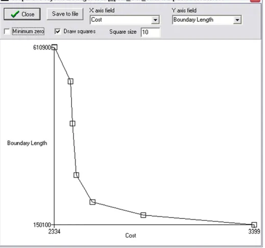
boundary length and target achievement. The scatter plots are very useful for calibration. For instance, ZC can plot boundary length against cost for various values of the BLM, a common method used for calibrating this parameter (Figure 5). Zonae Cogito also allows users to systematically explore the results of many Marxan runs using cluster analysis, the results of which can be visualized with dendrograms and non-metric multidimensional scaling plots.

Marxan, Marxan with Zones and Zonae Cogito are all free software and can be

downloaded from the Marxan website (http://www.uq.edu.au/marxan/), along with their

user manuals and the Marxan Good Practices Handbook.

Figure 5. Screenshot of the Zonae Cogito graphing functionality. Here a tradeoff curve has been plotted between

boundary length and cost, a common approach to calibrating the BLM parameter in Marxan.

2.7. ConsNet and Tabu Search

ConsNet is a software package for the selection of reserve networks, designed to solve the set cover problem (Ciarleglio et al., 2009). The most recent version can also solve the maximal cover problem. It is able to incorporate diverse spatial criteria in its

Conservation planning of threatened flora in northwest Iberian Peninsula: a comparison of two reserve selection tools

Conservation

planning of

threatened flora in

northwest Iberian

Peninsula: a

comparison of two

reserve selection

tools

Ricardo Reis Alves Soares Cardoso

Dissertação de Mestrado apresentada à

Faculdade de Ciências da Universidade do Porto em 13/12/2013

Ciências e Tecnologia do Ambiente

2013

planning of

threatened flora in

northwest Iberian

Peninsula: a

comparison of two

reserve selection

tools

Ricardo Reis Alves Soares Cardoso

Mestrado em Ciências e Tecnologias do Ambiente

Orientador

Coorientador

Resumo

Abstract

Acknowledgments

Table of Contents

List of Figures

List of Tables

List of Abbreviations

Chapter 1. Introduction and objectives

1.1. The decline of biodiversity and the role of protected areas

1.2. Systematic Conservation Planning

1.3. Objectives

Chapter 2. Reserve selection tools

2.1. Introduction

2.2. Formalization of conservation problems

2.2.1. Constrained optimization

2.2.2. Reserve network selection problems

2.2.3. Multicriteria analysis

2.2.4. Probabilistic data

2.3. Algorithms and software

2.3.1. Computational complexity

2.3.2. Heuristic algorithms

2.3.3. Metaheuristic algorithms

2.3.4. Optimal algorithms

2.4. Marxan and Simulated Annealing

2.4.1. Simulated Annealing and its implementation in Marxan

2.4.2. Marxan user interface

2.4.2.1. Input Files

2.4.2.2. Output files

2.5. Marxan with Zones

2.6. Zonae Cogito

2.7. ConsNet and Tabu Search