Pedro Themido Pereira Rodrigues
“Does Funding Liquidity help predict U.S Dollar returns?”
Dissertation written under the supervision of Professor Rui
Albuquerque
Dissertation submitted in partial fulfillment of requirements for the
MSc in Finance, at the Universidade Católica Portuguesa, April 2019.
Master Thesis in Finance
Abstract:
Predicting the future value of an exchange rate has been a long-standing challenge in economics. There is still no evidence of any model or technique that has consistently been proven to beat the random walk model. The current objective of this thesis is to check if there is a liquidity channel tied to banking funding that allows us to explain some part of the performance of currency returns. The present analysis focuses on the paper “Risk Appetite and Exchange Rates” by Adrian et al. (2015) where it is claimed that there is a statistically significant relationship between banks’ funding capacities and changes in exchange rates. This relation seems to be more prominent for currencies of more developed countries. In my analysis, the liquidity aggregates (Commercial Paper and Repo) also display some explanatory power, though less than in Adrian et al. Importantly, however, I show that using linear time de-trending as the authors do presents stationarity problems for both liquidity aggregates, especially for Repo volume. The statistical inference of the OLS results is therefore limited. Moreover, in the fitted models, adding a dummy variable and a dummy variable with interactions with the two liquidity aggregates, as in Adrian et al. (2015), reduces the individual significance of the coefficients’ estimates for the liquidity variables. Overall, my analysis casts doubt on the results obtained in Adrian et al. (2015).
Sumário:
A previsão do valor futuro de uma taxa de câmbio é um desafio de há muito tempo no campo da economia. Ainda não há provas concretas de nenhum método que seja capaz de bater o random walk model, na previsão das taxas de câmbio futuras. O objectivo desta tese é analisar se existe algum liquidity channel relacionado com o mecanismo de financiamento dos bancos que ajude a explicar alguma parte da performance do retorno das moedas. A análise desta tese debruça-se sobre o paper “Risk Appetite and Exchange
Rates” por Adrian et al. (2015), onde se afirma que existe uma relação estatisticamente
significativa e positiva entre a capacidade de financiamento dos bancos e os retornos da moeda em que é denominado esse financiamento. Esta relação parece mais forte entre moedas de países desenvolvidos. Na minha análise, os agregados de liquidez (Papel Comercial e Repo) também revelam algum poder explicativo, ainda que este seja menor que aquele apresentado em Adrian et al. (2015). Digno de nota é que o método de
de-trending (linear time de-trend), usado pelos autores, produz séries com problemas de
estacionariedade, especialmente para o valor do Repo. A inferência estatística é portanto limitada. Além disso, nos modelos ajustados, usar uma dummy variable e uma dummy
variable com interacções com os agregados de liquidez, como em Adrian et al. (2015),
reduz a significância individual para as estimativas dos coeficientes das variáveis de liquidez. Em suma, o meu estudo levanta dúvidas sobre os resultados encontrados em Adrian et al. (2015).
Acknowledgements:
I would like to thank Professor Rui Albuquerque for its guidance, patience, and vision on how to solve the different problems I have come across while doing this thesis. I also would like to thank Mary Fricker from Repowatch who has taught me the basics of the Repo market and has made easy the task of updating the Overnight Repurchase Agreement’s data series. I would also like to thank Tiago Castel-Branco for initiating me in computer coding particularly in the MATLAB programming language.
List of contents:
1. Introduction ... 1
2. The importance of foreign exchange currency markets: ... 4
3. The Dollar Standard ... 5
4. The Data ... 6
4.1 Basic Statistics ... 7
4.2 Correlation among currency pairs ... 10
4.3 Liquidity aggregates ... 11
4.4 Why do banks use Repos ... 15
5. Methodology ... 15
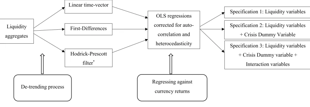
6. De-trending the liquidity variables ... 18
6.1 De-trending in respect to linear time vector ... 18
6.2 Stationarity... 20
7. Model Specifications ... 26
7.1 Comparing the different results: ... 30
8. Multi-lagged Regressions... 31
9. Conclusion... 33
10. Glossary... 35
11. List of abbreviations ... 37
List of Figures:
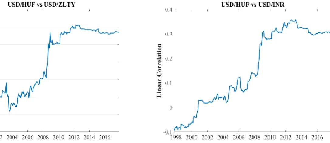
1. Linear Correlation between USD/HUF and USD/ZLTY, and USD/HUF and USD/INR (October 1997 until January 2018).
2. Primary Dealer’s Overnight Repurchase Agreements and Financial Commercial Paper Outstanding
3. Evolution of the “Market Share” between Repos and Financial Commercial Paper. 4. Scheme with the different combinations of de-trending the liquidity variables and the
several regression models.
5. De-trending the two liquidity variables with respect to linear time vector with a 48 training period observation
6. De-trended series as it is shown in “Risk Appetite and Exchange Rates, (2015)”.
7. Series of p-values of the Augmented Dickey-Fuller’s test (0 to 27 order lags of auto-correlation).
8. De-trending liquidity variables using first differences.
9. De-trending liquidity variables using the Hodrick-Prescott filter.
10. Relationship between the future monthly exchange rate of Australia and the three types of de-trending used in the Log Commercial Paper series.
11. Relationship between the future monthly exchange rate of Australia and the three types of de-trending used in the Log Repo Paper series.
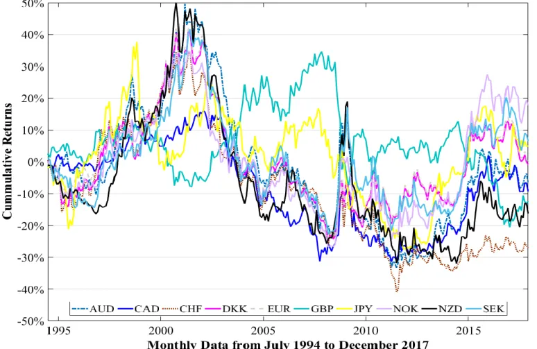
12. Cumulative returns of the U.S Dollar against developed countries’ currencies. 13. Cumulative returns of the U.S Dollar against emerging markets’ currencies.
14. t-statistics of the estimates for the coefficients of the Log (restricted model), when using linear time de-trending.
15. t-statistics of the estimates for the coefficients of the Log Commercial Paper (restricted model), when using linear time de-trending.
16. t-statistics of the estimates for the coefficients of the Log Commercial Paper (restricted model), when using first differencing.
17. t-statistics of the estimates for the coefficients of the Log Repo (restricted model), when using first differencing.
18. t-statistics of the estimates for the coefficients of the Commercial Paper (restricted model with a dummy variable), when using linear time de-trending.
19. t-statistics of the estimates for the coefficients of the Repo (restricted model with a dummy variable), when using linear time de-trending.
20. t-statistics of the estimates for the coefficients of the Log Commercial Paper (restricted model with a dummy variable), when using first differencing.
21. t-statistics of the estimates for the coefficients of the Log Repo (restricted model with a dummy variable), when using first differencing.
22. t-statistics of the estimates for the coefficients of the Log Commercial Paper (complete model), when using linear time de-trending.
23. t-statistics of the estimates for the coefficients of the Log Repo (complete model), when using linear time de-trending.
24. t-statistics of the estimates for the coefficients of the Log Commercial Paper (complete model), when using first differencing.
25. t-statistics of the estimates for the coefficients of the Log Repo (complete model), when using first differencing.
1. Introduction
There is a vast literature on predicting currency returns and limitless approaches that have been taken to try to explain currency movements. The modern study of exchange rates started with Mundell (1962) and Fleming (1964), (1968) who invented the known Mundell-Fleming diagram. Macroeconomic models were further developed by Niehans (1975), Mussa (1976), and Dornbusch (1976), among many others.
Empirical studies started with Frenkel (1976) but perhaps the most relevant paper until today, in the exchange rate literature is Meese and Rogoff (1983). In this paper, the authors use several known macroeconomic relationships and different econometric techniques in order to forecast one-period ahead exchange rates of a group of developed countries. Unfortunately, their study did not produce good results, not being able to beat the random-walk model. As Engel and West (2005) posit:
“Our theories state that the exchange rate is determined by fundamental variables, but floating exchange rates between countries with roughly similar inflation rates are in fact well approximated as random walks. Fundamental variables do not help to predict future exchange rates.”
Surely there are other ways to look at the problem, instead of just looking for monetary aggregates and macroeconomic variables to try to predict the future monthly currency return. Purchasing-Power parity models and trade-balance models were proposed by academia to try to understand the phenomena. Rapidly models started to get more complex with agents having different preferences regarding their liquidity constraints and their portfolio allocation needs. The goal was no longer to beat the random walk but to explain some part of the variations in currency moves. Factor models of exchange rates started to appear: for example, Engel et al. (2014) try to encompass the long-run effect of Purchasing Power Parity and monetary aggregates together. The field of study is vast and as more information is made available, more approaches appear.
The paper by Adrian et al. (2015) “Risk Appetite and Exchange rates” (henceforth referred as Adrian et al. (2015), predicts a relationship between a banks’ ability to expand their balance sheets’ liabilities and the out-of-sample moves in currency returns against the U.S Dollar. It concludes that there is a statistically significant positive relationship between expanding liabilities in U.S Dollars and a U.S Dollar appreciation.
The objective of this Master Thesis is to reassess the conclusions of the paper by replicating the results and analyzing them under different assumptions. I wish to confirm that the increase in short-term liquidity aggregates can indeed forecast some part of the variation of the future’s spot exchange rate return.
The first part of this thesis tries to understand how the funding mechanism works. Adrian et al. (2015) claim that it is the structure of how banks deploy their funds across their international branches that create imbalances in the demand and supply of a given currency pair. The centralized funding model of banks can impact the currency markets because short-term funding is required to do these cross-border transactions. Besides this, the short-short-term funding capacity of a given bank depends on its capital ratios. Banks will have to optimize their decisions of funding to their capital constraints and will have to “play” in a given market environment to decide whether it is optimal or not to deploy the funds across its subsidiaries at a given time. This optimization problem is not studied in the scope of this thesis. It is only studied if it is possible to infer if the preliminary conclusions that were drawn by Adrian et al. (2015) can be done with the data currently available. There are however some limitations in the data presented as it will be mentioned in chapter two.
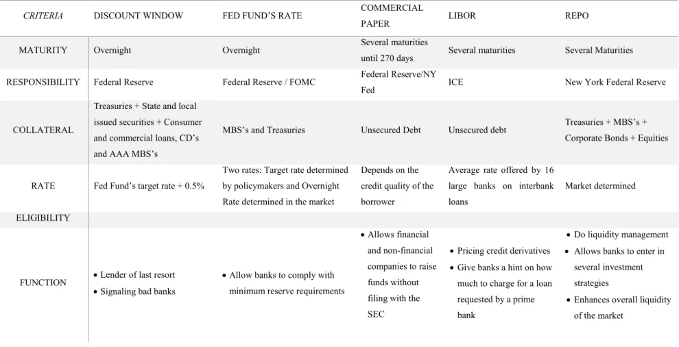
Usually, banks fund their daily activity managing very short-term loans. Like any other type of loan, it is meant to be repaid but it can be generally “rolled-over” indefinitely if the credit quality of the agent asking for the loan is maintained or if the creditor does not require the payment of the loan´s principal due to a severe liquidity crisis. There are several mechanisms whereby banks can get their liquidity from, being the main facilities the Repo Market, the Federal Reserve Discount Window, inter-bank lending, the Federal Reserve Fund’s rate and the Financial Commercial Paper facility among others. Table 1 in the Appendix describes the main features of these funding facilities.
The authors1 of Adrian et al. (2015) use the Overnight Repo Market and the Financial
Commercial Paper as liquidity variables in order to predict the one-period-ahead returns of twenty-three currencies, both from developed and emerging markets countries between the months of January of 1993 to December of 2014. This sample comprises roughly 264 monthly observations of data for currency returns and for both liquidity aggregates. The results obtained by the authors are remarkably good and seem to indicate that whenever there is an expansion of the dollar-denominated liquidity aggregates, the U.S Dollar tends to appreciate.
The second part of the thesis broadly discusses the importance of the foreign exchange markets. In section three the properties of the U.S Dollar as the dominant currency are approached. In part four basic statistics of the U.S Dollar are presented against twenty-six cross rates, and the liquidity aggregates are introduced. Part five and six present the methodology used as well as the de-trending methods applied to the data and the respective conclusions regarding the stationarity of the de-trended series. The linear time de-trending performed on the
liquidity aggregates fail the unit-root stationarity tests, unlike de-trending the series using first differences or using the Hodrick-Prescott filter. Part seven discusses the results of the one-month ahead OLS regressions. The explanatory power of the regressions is much lower than the results presented in Adrian et al. (2015) for linear time de-trending, and get even worse when the dependent variables are de-trended using the Hodrick-Prescott filter. Despite the fact the explanatory power of the regressions is similar whether linear time de-trending or first differencing are applied to the Logs of the liquidity aggregates, the different signs of the estimates for the two coefficients of the liquidity aggregates in the two de-trending methods is not consistent with any economic conclusion drawn by Adrian et al. (2015).
Moreover, adding a dummy variable (related to the financial crisis’ starting year) and interaction terms with the liquidity aggregates did not produce the desired results for the current data series. In part seven it is also discussed possible reasons that might explain the different results. Part eight checks for alternative lags of the regressions where results might be similar to the ones in Adrian et al. (2015). Part nine summarizes the main findings of the present study, namely that for some developed currency pairs, the restricted model (the model specification where only the two liquidity aggregates are included in the regression) is better than the complete model in explaining future U.S Dollar returns.
2. The importance of foreign exchange currency markets
The foreign exchange market is the most liquid and largest market in the world with an average daily volume of 5 trillion dollars, which makes it twenty-five times bigger than equity markets. Institutional investors, Central banks, Investment banks, Hedge funds, Currency speculators, and Retail traders, they all operate in this de-centralized market over twenty-four hours of the day, around the globe.
There are several currency regimes, of which the most popular ones are the conventional peg, the floating regime and the free-floating regime (IMF, 2017)
The most liquid currencies and the most traded ones are from developed countries which use a free-floating currency regime. The main advantages of having a developed and liquid foreign currency market are: the possibility agents have to enhance trade relationships between countries, therefore contributing to price convergence; the availability of moving capital flows in a timely manner; the opportunity to hedge cross-border business risks derived from currency fluctuations; and, finally, the availability banks and companies have to fund themselves in foreign currency at a lower cost (currency swaps).
In a hypothetical world where there was only one single currency and under perfect competition and information, all the same goods, services, and means of production should cost the same, since differences in prices would be sooner or later arbitraged. Since there is no single currency, (there are at least more than 180 currencies accepted as legal tender), and there are many trade barriers, such as taxes, tariffs, and inflation among others, it is natural that in different countries prices for the same goods, services and means of production will differ.
The main objective of a liquid and open currency market is to come as closer as possible to the utopic idea of a single currency, in order to mitigate the effects of negative externalities to trade that national governments and other forces impose.
3. The Dollar Standard
The U.S Dollar is by far the most traded currency in the world accounting for 87.1% of overall traded currencies. In 2016 it averaged roughly 4.4 Trillions of Dollars traded on a daily basis according to the Bank of International Settlements’ Triennial Report, BIS (2016). The traded volume comprises Spot market transactions, Outright Forwards2, Foreign Exchange
Swaps, Currency Swaps3, Options, and other highly leveraged products. This volume includes
both long and short positions.
There is a combination of factors why the U.S Dollar is the dominant currency: size of the U.S economy, financial innovation in the U.S financial system, market liquidity, network externalities applied to global trade4…etc. But perhaps the organization of the banking system
is probably the most important reason.
The way the dollar become the reserve currency paved the way to the dollar standard. This dominance gave its first steps when the Federal Reserve was created, and continued to grow during the two World Wars. The Federal Reserve was a determinant factor in establishing the dollar as the world reserve currency, enhancing market liquidity. When all other countries were not allowing convertibility to gold, the United States preserved gold convertibility. This made the U.S Dollar expand as a means of payment and as a unit of account between private parties, Eichenbaum (2005). The period post-World War II was one of dominance for the dollar, as other areas as Europe or Japan were struggling to recover from the war and were tightening their capital controls resulting in having very illiquid securities market in these countries. This sole fact made global banks to fund their activities mostly in dollars because they could unwind their positions whenever they wanted, reducing liquidity risk as much as possible. By the late 1990s as capital controls started to being lifted in most of the countries, the US Dollar was already the dominant reserve currency, the currency for settling transactions and for trading securities in financial markets since the late 1970s.
2 An outright forward is a forward currency contract that locks in an exchange rate for a specific delivery date and a specific amount. An
outright forward contract protects an investor, importer or exporter from changes in the exchange rates. Foreign exchange forward contracts can also be used to speculate in the currency market. (Source: Investopedia)
3 Foreign exchange swaps are the primary means through which global banks manage currency mismatch between their assets and liabilities. A
swap contract enables a bank to exchange local currency for U.S Dollars at the current exchange rate, while agreeing to reverse the transaction, that is, exchange U.S dollars back to local currency at the forward exchange rate. Maturity may vary between three months and several years through OTC. Counterparties typically post collateral, which is adjusted depending on movements in currencies, Ivashina,V., et al. (2012)
4 “Network externality has been defined as a change in the benefit, or surplus, that an agent derives from a good when the number of other
agents consuming the same kind of good changes. As fax machines increase in popularity, for example, your fax machine becomes increasingly valuable since you will have greater use for it. This allows, in principle, the value received by consumers to be separated into two distinct parts. One component, which in our writings we have labeled the autarky value, is the value generated by the product even if there are no other users. The second component, which we have called synchronization value, is the additional value derived from being able to interact with other users of the product, and it is this latter value that is the essence of network effects.” (Leibowitz, S. Morgulis, S.) https://www.utdallas.edu/~liebowit/palgrave/network.html
4. The Data
All the data presented in this thesis was retrieved from Thomson Reuters Datastream, from the New York Federal Reserve site, from the Board of Governors of The Federal Reserve site and from Repowatch.com. The data was then treated using Matlab programming language.
The set of data comprises monthly observations from July 1994 until December 2017. The present thesis aims to analyze twenty-six cross-rates, using the US Dollar as the base currency. The sample size has 282 monthly observations.
In the original paper, the time span of the sample goes from January 1993 to December 2014. Unfortunately, the observations from January 1993 to June 1994 are no longer available in the New York Fed website, for the Overnight Repo (henceforth denominated as Repo). The observations that are possible to retrieve from the New York Federal Reserve for the Repo aggregate only begin in 1998. The observations from mid-1994 until 1998 presented in this thesis were gathered with help from Repowatch.com.
The authors of “Risk Appetite and Exchange Rate” don’t specify if the time series are seasonally adjusted or not. More importantly, a major reclassification was done by the Federal Reserve board in the way Financial Commercial Paper is counted from 2006 to the present day.
In the Federal Reserve’s website, there are instructions on how to adjust the old methodology to the new one, in order to have a comparable data series5. In the present thesis,
the series of the Outstanding Financial Commercial Paper aggregate was treated using the adjustment method mentioned above. In the original paper, it is not clear whether the authors have used the reconciliation method proposed by the Federal Reserve or another type of method.
The cross-rates that were studied were between the U.S and two groups of countries. A group of developed countries (Australia, Canada, Denmark, Euro-area, Great-Britain, Japan, New Zealand, Norway, Sweden, and Switzerland), and a group of countries considered as emerging markets (Bangladesh, Brazil, Hong Kong, Hungary, Indonesia, India, Malaysia, Mexico, Philippines, Poland, Singapore, Taiwan, Thailand, Turkey, South Africa, and South Korea). The developed countries studied are the ones used by the authors in their paper while the emerging markets group is not quite the same.
5 In this web address: https://www.federalreserve.gov/releases/cp/about.htm it is broadly explained the changes that have been done in order
4.1 Basic Statistics
In Table 2 and Table 3 of the Appendix, the descriptive statistics are presented for the monthly currency returns (where returns are defined as 𝑆𝑡
𝑆𝑡−1− 1)
6 of the U.S Dollar against the
most developed countries’ currency pairs and emerging markets currency pairs, respectively. It is observed that monthly returns are centred on their means and it is not possible to reject the null hypothesis of zero-mean returns for all developed countries considered. The idea that exchange rates’ returns (as most of the financial series) don’t follow a Normal distribution, can be seen in the critical values presented for the Jarque-Bera’s test, that rejects the null hypothesis at 1% significance level for nine out of ten developed countries and for all emerging markets. Positive skewness is exhibited for almost all currency pairs. Financial series usually have negative skewness. This is given by the fact that negative returns are usually greater in magnitude than positive returns, the stylized fact of gain/loss asymmetry, Cont (2001).
However, this stylized fact does not seem to occur for the U.S Dollar, where positive returns are usually larger than negative returns against fifteen of the sixteen emerging markets considered and for seven of the ten developed countries.
Kurtosis is also greater than 3 which goes along with financial literature that states that the distribution of returns of financial time series has higher probability mass on their extreme values, meaning that extreme events tend to happen with more probability than the Normal distribution would predict.
Regarding the performance of the U.S Dollar against emerging markets’ currencies, it is possible to state that the normality hypothesis is rejected much more strongly. The distribution of returns besides not being symmetric (all emerging markets present a very positive skewness) and having very fat tails, is also not centred on zero for eight of the sixteen currency pairs (as it is possible to see for the significance levels presented in Table 1 for the mean returns).
Comparing the two groups of countries one can state that there are two distinct patterns. Developed countries’ currencies tended mostly to appreciate against the Dollar, and currencies from emerging markets tended to devalue immensely. The simple standard deviation of returns of the two groups of currencies is also completely different. Emerging markets’ currencies register a much higher standard deviation than developed countries. This fact goes along with
6The authors of Adrian et al. (2015) claim that the difference between using Log Returns or Simple returns was insignificant, so it is used
financial theory since if one sees holding a given currency as holding an asset, it is understandable that riskier assets have much more variability than safer assets.
Because emerging markets have generally more risks than developed countries (less integration in the international financial markets which leads to less liquidity of their currencies, more country default risk makes currency premiums higher for these currencies), it is normal that investors will require a higher compensation for holding investments denominated in exotic currencies. However this might be an explanation, this does not fully explain why only one (in the emerging markets group) in sixteen countries has seen its currency appreciated against the US Dollar, and most of the other countries (11 out of 16) have seen their currency devalued more than 50% in roughly twenty-three and a half years as it is seen in Table 2 of the Appendix. In October of 2011, some economists in one of the IMF Staff discussion notes alerted for the possible risks and rewards of emerging markets liberalize their capital flows. In this brief discussion citing other sources, namely the BIS triennial report already mentioned above, they said that probably by 2035 the US Dollar would be substituted by other currency as the dominant one in global transactions and as the major reserve currency held by Central banks. They argued that at that time there were some currencies that could become serious players in international trade such as the South African Rand (ZAR), the Brazilian Real, the Indian Rupee (INR), the Chinese Yuan (RMB), and the Russian Rouble (RUB) (the last two are not studied in this thesis).
The authors of this staff discussion argue that would be beneficial for Central banks to have a more diversified portfolio when managing their reserves’ allocations. This could be a way for Central banks to reduce exposure to currency risk, given that they would be investing in uncorrelated currencies reducing, therefore, their Value-at-Risk.
According to the Triennial Report of BIS, Central banks had been buying more reserves from exotic currencies in most recent years. From 2004 to 2011 the share of exotic reserves rose from 2.4% to 7.1% of the total reserves held by Central banks and then decreased in 2015 to 4%. The overall tendency of Central banks to increase their exposure to exotic reserves should have lead to an appreciation of the currencies of these countries. The sharp depreciation of these currencies has to be explained by other factors.
Often there are three main channels where it is possible to look in order to measure the use of given currency: in the buying and selling of reserves by Central banks, on the invoicing and settlement of international transactions and, finally, in the volumes traded in foreign exchange markets (IMF, 2011).
The almost non-existence of derivative contracts to hedge positions in exotic currencies and very wide bid-ask spreads that market-makers demand to trade these currencies might explain why the volume traded of exotic FX currency pairs is so low. Although reserves held by Central banks may have been in an ascending trend, the U.S Dollar continues to be the reference currency for invoicing international transactions, and it is the only currency used to price all the commodity futures that exist.
Moreover, most of emerging market countries have faced serious inflationary pressure in the last twenty years making investors reluctant in holding currency from these countries.
These reasons among many others might explain the enormous appreciation that the dollar has registered against exotic currencies.
4.2 Correlation among currency pairs
The different levels of correlation between currency pairs of developed markets and emerging markets should not be disregarded. Between emerging countries, there is much less linear correlation than in developed ones (Tables 3-a and-3 b). Less financial integration and undeveloped financial systems lead to poor capital mobility, what might explain the little degree of linear correlation. On the other hand, because capital mobility is easier in developed countries, they are much more dependent on each other in the sense that there are no other markets with the adequate structure or size to absorb the wealth generated in these countries.
However a remark must be done: correlations are not steady. The correlations presented in Table 3-a and Table 3-b are a product of twenty-three years of data. Some countries may have registered an increase in correlation signaling higher financial integration but they still present low levels of correlation for the entire sample size.
A good example is the evolution of the degree of linear correlation between the U.S Dollar/Hungarian Florint (USD/HUF) and the U.S Dollar/Polish Zloty (USD/ZLTY) cross rates (Figure 1). The correlation between these two currency pairs became much more significant after the 2007-08 crisis. The correlation between the USD/HUF and U.S Dollar/Indian Rupee (USD/INR) present the same tendency, and the same pattern is verified for the cross-correlations between most of emerging markets’ currency pairs.
4.3 Liquidity Aggregates:
Repo
What is a Repo? The repurchasement agreement’s market only started to grow in the late eighties when a set of legal reforms were put in place to better accommodate for default risk of the counterparty, and computer advances made the lending and repurchase of securities much easier and safe (however the first Repo transaction registered dates back to 1917).
A repo can be seen in two ways: as a collateralized debt contract or as a mean for securities lending.
The basic structure of a Repo contract as a collateralized debt contract is a trade in which both parties agree to exchange securities for cash, for a given period of time. This agreement comes with the promise of the agent who sells the security for a given price for a given amount of cash, to buy back that security in the future from the cash lender at a pre-determined higher price.
The difference between the pre-determined price of buying-back the security and the price of selling is the gain that the lender of cash makes. The securities pledged are often the most liquid possible so that if bank A (the borrower of cash) can’t meet its promise of buying-back the securities at the pre-determined higher price, the counter-party (usually a Money Market-fund) can quickly sell those securities in the market and get the cash that was supposed to be delivered by bank A. The repo rate7 reflects the liquidity of a given collateral and the ability for
the counter-party to buy-back that collateral in the future date. Collateral accepted by the New York Fed goes from very liquid Treasury-Bills to not so liquid Mortgaged-backed securities.
One of the big problems of studying the Repo Markets is that there are no standard measurements across different institutions to determine its true size. The ICMA foundation estimates that the U.S Repo Market ranges between $5 and $10 trillion, whereas the Federal Reserve of New York reported that the U.S outstanding Repo market8 amounts to $4.6 trillion.
On the other hand, Sifma9 reports a value of only $2.6 trillion and the Federal Reserve reports
the lowest value, $2.2 trillion, Baklanova et. al (2015).
7 The repo rate is usually calculated using the (P
t-P0)/P0*(Maturity of repo contract)/365 formula. Where P0 is the cash paid by the security’s
borrower at the inception of the trade and Pt is the pre-determined price paid by the security’s lender to buy-back the securities. Example:
Bank A needs funding of $50M and has $50M in T-Bills. The bank goes to a Money Market Fund and “sells” the $50M T-Bills with the promise to buy the securities back at $52.5M in three months. The repo rate will be $2.5M/$50M*(120/365) which is roughly 1.64%.
8This amount only comprises the Repo activity between the New York Federal Reserve and the group of Primary dealers. 9Source: https://www.sifma.org/resources/research/us-repo-market-fact-sheet-2017/
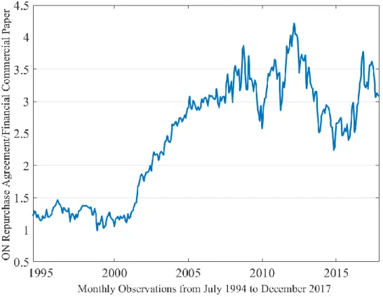
Although there are multiple estimates for the value of the U.S Repo market, the data that was considered was taken from the Federal Reserve of New York. The series seems to match in levels, the series used by the authors in Adrian et al. (2015), (Figure 2).
The problem with this data is that it only includes transactions between the Federal Reserve of New York and Primary U.S Dealer banks (according to ICMA the transactions with Primary Dealer banks may account for as much as 90% of the U.S total Repo market), and it only includes “Overnight and Continuing Repos”.10
The New York Federal Reserve distinguishes between “Overnight and Continuing Repos” and “Term Repos”. The first category comprises contracts that are due in one day but are technically “rolled-over” indefinitely if necessary, and the second comprises contracts that have a pre-specified maturity that goes no longer than two years. Term Repos have significant importance in the U.S Repo market accounting for almost one-third of it. The data is therefore incomplete and it might lead to misleading results.
Although the overnight LIBOR11 rates registered the lowest levels after 2009, Figure 2
shows that “Overnight and Continuing Repos” didn’t return to pre-crisis levels in the following years. Intermediation of the Repo Market through the introduction of the Tri-Party Repo mechanism made the costs of Repo funding to increase, which made banks to migrate for other types of instruments, such as Collateral swaps, BIS (2017).
10The Overnight Repurchase agreement aggregate cannot be considered truly as an outstanding value since it is a flow and not a stock. It does
not make sense to add-up the values of several days of overnight Repo’s to get a monthly value.
11 The London Interbank Offered Rate (LIBOR), is the short-term rate that major banks use to fund themselves in the interbank market. The
rate is set as the average rate submitted by 16 banks on a daily basis. Several maturities and currencies are available. LIBOR is usually used to price debt instruments and derivatives and it is often regarded as a major indicator of liquidity conditions.
Figure 2- Primary Dealer’s Overnight Repurchase Agreements and Financial Commercial Paper Outstanding. The correlation between Logs of Overnight Repo’s and Outstanding Financial Commercial Paper is 0.56 for the entire period
Financial Commercial Paper Outstanding
Commercial Paper is a quick and easy form of funding in the short-term unsecured debt markets. There is a wide range of maturities, (from 7-day maturity to a maximum of 270 days), however the average maturity of all financial commercial paper is below 30 days. Funding through the commercial paper facility does not require SEC approval. The financial commercial paper aggregate takes only into account unsecured debt issued by the U.S financial private sector. This type of security is used to face short-term liquidity management and it is often more expensive than Repo transactions because they are uncollateralized loans. This type of security is issued mainly by prime-banks which counterparties consider very trustworthy or by very distressed banks that cannot place their liabilities on secured debt markets and are subject to higher premiums. The most common holders of financial commercial paper are money-market funds, wealthy investors, corporations and other banks.
In Figures 2 and 3 is possible to see that Financial Commercial Paper co-moved with Repo between 1994 until 2002 (with different growth rates); then, from 2002 to 2008, the Repo aggregate grew immensely and the Commercial paper decreased, and from 2008 to today the Overnight Repo aggregate has trended between almost 2.5 and 4.5 times the Commercial Paper
aggregate. Looking at figure 3, it is possible to perceive that during the crisis, the Repo aggregate decreased more than the Commercial Paper. Nonetheless, currently, the Repo Market is much bigger (approximately three times bigger) than Financial Commercial Paper.
Figure 3 – “Substitution” of Financial Commercial Paper by overnight re-purchase Agreement
Comparing these two aggregates is not very reasonable since, economically speaking, Overnight Repo is a flow and Outstanding Financial Commercial Paper is a stock. Nonetheless, it is possible to perceive a general trend that Repo is dwarfing commercial paper as a mean of funding for the financial industry.
4.4 Why do banks use Repos
Besides being a very liquid market where banks can easily access funding and do liquidity management, Repo transactions are suitable to raise money for a wide range of investment strategies such as carry-trades, yield-curve trades, relative-value trades, and spread trades, (BIS 2017). It also suits the needs of banks which find unsecured debt too costly or are having troubles raising cash in unsecured markets. Moreover, Repo transactions increase the liquidity of the overall market as the agent that receives the security can do a Repo of a Repo, giving the security as collateral to raise money elsewhere.
5. Methodology
5.1 De-trending liquidity aggregates in respect to a linear time trend:
The methodology used was the following: first, both Logs of the liquidity aggregates were regressed in respect to a linear time vector of n observations, t= [1, 2, 3…n] (as the authors have done).
A training period of four years (48 observations) was considered in order to calculate the coefficients of the regression in:
LogRepot = α + βt + et (1.1)
With the coefficient estimates, the residuals were calculated subtracting the fitted values from the observed values for the first 49 periods.
𝑒̂𝑡= LogRepot - (𝑎̂ + 𝛽̂t) (1.2)
After this step, several regressions, each one with one more observation than the preceding regression (expanding window), were made in order to calculate the residuals for the immediately following month. In the final step, the first 281 observations were used in the regression and estimated coefficients were used to de-trend the 282nd observation. The same
procedure was applied when de-trending the Log of Commercial Paper. De-trending in this fashion eliminates any look-ahead bias.
The resulting de-trended series was tested for stationarity using the standard tests: Dickey-Fuller, Augmented Dickey-Fuller, Philippe-Perron and the KPSS test.
Besides de-trending the data with respect to linear time trend as in Adrian et al. (2015), the Logs of the two liquidity aggregates were also de-trended using first differences and the Hodrick Prescott filter, and then tested for stationarity.
The following step was to consider the twenty-six currencies of the countries studied and calculate the monthly returns for the period between August 1994 until January 2018 (282 observations). These series of returns were considered as the dependent variable in OLS estimation.
Several model specifications were taken into account. First, the dependent variable (the monthly returns) were regressed only against the two de-trended liquidity aggregates. The series of the liquidity aggregates considered in the regressions were lagged at one month for the first difference de-trending and for the Hodrick-Prescott filter and lagged at one and two months for the linear-time de-trending. For this model specification, only the most developed countries were considered.
A financial crisis dummy variable was introduced in a new set of twenty-six regressions (developed countries plus the emerging markets), with the three types of de-trending. The last specification used was the one used in Table 1 of Adrian et al. (2015) and accounts for the possible interaction effect between the financial crisis dummy and the liquidity aggregates. The Hodrick-Prescott filter was not considered for this last model specification since it presented very poor results in the previous model specifications. The OLS estimates were corrected for auto-correlation and heterocedasticity using the Newey-West correction at four lags, as Adrian et al. (2015) do.
In the last step, the same model specifications are run using lagged regressions of the explanatory variables (up to thirteen lags).
Figure 4- Scheme with the different combinations of de-trending the liquidity variables and the several regression models.
OLS regressions corrected for auto-correlation and heterocedasticity Liquidity aggregates Linear time-vector First-Differences Hodrick-Prescott filter*
Specification 1: Liquidity variables Specification 2: Liquidity variables
+ Crisis Dummy Variable Specification 3: Liquidity variables
+ Crisis Dummy variable + Interaction variables
De-trending process Regressing against
currency returns
6. De-trending the liquidity variables
6.1 De-trending in respect to linear time vector
The liquidity aggregates were de-trended with respect to a linear time vector, as in Adrian et al. (2015). In Adrian et al. (2015) it is not specified if it is used a rolling or an expanding window in order to get the residuals that will later be used as independent variables for running the one-month ahead regressions. Also, the authors do not specify the number of observations that are used as a training period.
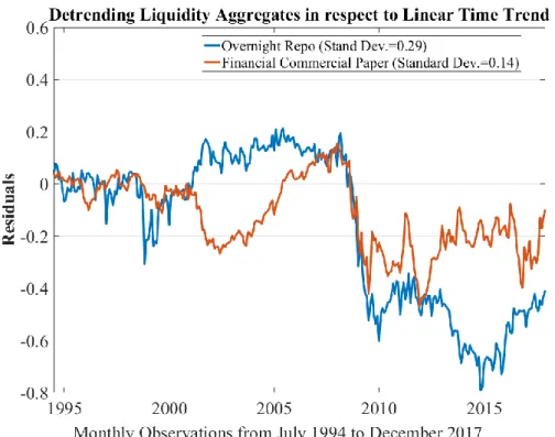
In this thesis, the expanding window method was chosen and 48 monthly observations were used as a training period. Figure 5 and Figure 6 show some differences between the de-trended series that were obtained in this thesis and the series in the paper.
However the two series seem to exhibit a similar behavior from the beginning of the sample until the period of the crisis in 2008 as can be seen in the graphs of the next page, it seems that after 2008 the de-trended Log Commercial Paper starts to behave differently, showing a different range of values: the de-trended Log Commercial Paper does not take so negative values in Figure 5 as it takes in Figure 6. This contributes to a smaller sample variance of the time series for the sample data of this thesis. Also, the difference between the two de-trended series starts to increase in mid-2012 in Figure 5, whereas the difference between the two series only increases in the graph of Figure 6 after 2015.
By contrast, the de-trended Log Repo’s behavior matches almost perfectly in both graphs. This fact brings up the question that the different behavior of the de-trended Log Commercial Paper showed in the two graphs might be due to differences in the measurement of the aggregate itself (already mentioned above), rather than differences in the de-trending process (expanding window vs rolling window or the number of observations used as a training period).
Another aspect worth looking for is the degree of linear correlation between the two aggregates in both graphs. In the paper, the authors report that the correlation between the two series is -0.73 for the period between 1993 until 2007 and -0.33 between 2010 and 2015. For the data of this thesis that goes from mid-1995 (the earliest observation that is possible to get) to 2007 the correlation of the two series is -0.17 and for the period between 2010 and 2015, the correlation is -0.54.
More things can be said about the graphs of Figure 5 and Figure 6, namely that the two series in both graphs do not seem to follow a stationary process, at least in variance terms (the magnitude of changes seems to be increasing along time). Also, the two liquidity aggregates seem to present a mild downward trend across the sample size not reverting to their mean.
Moreover, it seems there is a structural break in the behavior of both aggregates before and after the financial crisis of 2008.
The statistical inference made hereafter can be compromised if these problems are confirmed.
Figure 5 – De-trended liquidity aggregates of Log of Repo and Log of Commercial Paper with the data presently available
Figure 6 – De-trended liquidity aggregates of the Log of Repo and the Log of Commercial Paper as it is in the replicated paper. Source: Adrian et al. (2015)
6.2 Stationarity
A data generating process that is weakly stationary has a finite and constant mean, variance and auto-covariances. It means that the observed mean, variance and auto-covariance are independent of the sample size. Working with real sample data, some tests can be done in order to assess if a series is stationary or not. There are several classes of tests that can be performed in this current data sample to address the problem of stationarity vs non-stationarity.
The class of tests performed in this thesis are called unit-root tests and are the most commonly used when testing the stationarity hypothesis.
A unit-root process is a data generating process whose first difference is stationary (yt = yt-1 + stationary process).
The central idea of most of these tests is to fit an AR (1) model to the data to see if the slope of the model obtained is equal to or lower than 1.
yt = δyt-1+et, et is i.i.d with mean 0 and variance σ2 (1.3)
If the |δ| >=1 then the series will be growing boundlessly and as a result, it will not be stationary. If |δ| < 1 then the series is stationary and will always go back to its mean value.
The problem of these type of tests is to assume a given data generating process, in this case, an Auto-Regressive process of order 1.
The Phillips-Perron test assumes as a null hypothesis that the data follows a random walk with δ = 1, which is a non-stationary process.
yt = yt-1+et, with et following a white noise process (1.4)
The alternative hypothesis is that the data follows an AR (1) as described in (1.3) with δ
< 1
The Philips-Perron test performed on the trended data series (using linear time de-trending) does not reject the null hypothesis and the estimated values for the coefficient δ are 0.99 and 0.97 for the Repo and for the Commercial Paper, respectively. Also, the R-square of the regression of the series on a random walk is 0.97 for the Repo and 0.91 for the Commercial Paper. It is reasonable to think that both aggregates behave like random walks, and if they do, they are not stationary. The Phillips-Perron test was also run assuming that under the null hypothesis the series follows a random walk with drift and a random walk with a time trend.
Once again the test failed to reject the null hypothesis for both liquidity aggregates meaning that linear time de-trending does not produce stationary series.
The augmented Dickey-Fuller’s test is also performed on the two liquidity aggregates because, although the Phillips-Perron corrects for auto-correlation and heteroscedasticity through Newey-West estimates, Davidson and MacKinnon (2004) report that the test performs worse in finite samples comparatively with the augmented Dickey-Fuller test. The test is similar to the Philips-Perron test with additional regressors for lagged differences of the dependent variable but assumes that the error terms (et) are homocedastic. Under the null hypothesis, that is δ = 1, it is considered that the series follows the following model expression:
yt = yt-1 + β1Δyt-1 + β2Δyt-2 +…+ βpΔyt-p + et,12with et being a white noise process (1.5)
against the alternative hypothesis of δ < 1:
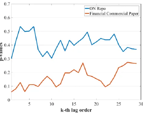
yt = δyt-1 + β1Δyt-1 + β2Δyt-2 +…+ βpΔyt-p + et (1.6) The problem with this test is that the lag order has to be selected, and there is no clear rule to do that. Schwert (1989) proposes to start at a defined lag of order pmax given by the equation pmax = [12 (T/100)1/4], where T is the number of sample observations. If the t-statistic of the coefficient of order pmax is statistically significant, the lag order is appropriate. If not, the lag order should be reduced until the coefficient become significant. For the data set of this thesis, it was first used a lag of order 0 which corresponds to the simple Dickey-Fuller test, and the Dickey-Fuller test with 1 to 27 lags, which is the lag order corresponding to the rule of pmax defined by Schwert and adequate for this thesis sample size. The simple Dickey-Fuller’s test does not reject the null hypothesis (Table 5) as expected since the Dickey-Fuller’s test is identical to the Philips-Perron test, without being corrected for auto-correlation or heterocedasticity. Figure 6 reports the p-values of the Augmented Dickey-Fuller test with 1, up to 27 lags. The test fails to reject the null hypothesis at a 5% significance level. Therefore, it is not possible to reject the hypothesis that the linear time de-trended series follows an integrated process of order p and therefore the series is non-stationary.
12 This Δ operator performs the first difference of the variable, that is Δy
Figure 7 – The graph presents the p-value for several lags of auto-correlation for the test hypothesis that δ = 1. The augmented Dickey-Fuller test fails to reject the null hypothesis that the de-trended series follows a random walk process. The minimum p-value registered between the two series is 0.06 at lag order 1 for the Commercial paper aggregate.
The KPSS test, another test to assess if a series has a unit-root and therefore is non-stationary, reverses the decision of the hypothesis testing. If the test rejects the null hypothesis, there is evidence of a unit root. The KPSS assumes under the null hypothesis that the series is trend stationary13.
yt = ct + αt + u1,t (1.7)
ct = ct-1 + u2,t (1.8)
The α is the trend coefficient, u1,t is a stationary process and u2,t is white noise with mean 0 and variance σ2.
The auto-regressive term enters in equation (1.7) through the variable ct and the null hypothesis is that σ2 = 0. If this is the case this means that c
t is constant and behaves like an intercept in equation (1.7). By contrast, if σ2 > 0 equation (1.8) becomes the standard random walk model, introducing, therefore, non-stationarity in the main equation (1.7).
So H0: σ2 = 0 vs Ha: σ2 > 0 is a one-sided test and rejecting the null hypothesis means that
the series rather than being trend stationary is integrated of order 1.
13 A trend stationary process is a process which when its mean is estimated and removed, the resulting residuals
For the two datasets studied, the KPSS test rejected that the Overnight Repo is a trend stationary process at 1% significance level and does not reject the null hypothesis for the Financial Commercial Paper at a 5% significance level. So the test concludes that the Overnight Repo has a unit-root and it concludes that cannot be rejected that the Commercial Paper follows a trend stationary process.
The results of the tests for stationarity performed on the liquidity aggregates in this thesis do not imply necessarily that the series used in Adrian et. al (2015) in their regressions are non-stationary. In Figure 4 and 5 it can be seen that the same aggregates behave differently. This different behavior might be because of the different time period covered in both samples, the different de-trending method used by the authors (the authors might have used rolling regressions instead of expanding window in order to get the residuals for the de-trended series) or because the initial levels of the liquidity aggregates are not measured in the same way, since it was already reported that major changes were done in the way Financial Commercial Paper aggregate is measured since 2006. This being said, a remark must be made that the Repo aggregate which is the series that seems to exhibit an identical path in both graphs, is also the series in which the non-stationarity hypothesis is more evident in the realized tests.
Nelson and Kang (1984) state that de-trending a series in respect to a linear time function, assuming that the series is a trend stationary process when in fact it is a difference stationary process will inevitably produce a series of non-stationary residuals. If the initial series is a DSP, then the appropriate de-trending method is to take differences of order k until the residuals are stationary.
Taking the first differences of the Logs of the liquidity aggregates is enough to make Repo and Commercial Paper series stationary as it is seen in figure 5 and in table 6 (in the Appendix), where the Phillips-Perron, augmented Dickey-Fuller and KPSS test results’ are presented. All the tests show evidence of stationarity for the differenced series of Log Repo and Log Commercial Paper.
The de-trended data in respect to a linear time trend it is not suitable for making sound statistical inference since Granger and Newbold (1974) state that using non-stationary series in regressions may result in spurious regressions, with misleading high R-squares and statistical significance of the regressors. However this might be the case, the regressions using these non-stationary series are still performed, in order to compare the results obtained with the results presented in Adrian et al. (2015).
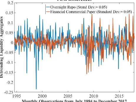
De-trending using First Differencing
Using this type of de-trending makes both series look like white noise processes with mean zero and constant variance. Differences are taken from the Logs of the liquidity aggregates:
ΔYt= Yt - Yt-1 (1.9)
This transformation makes the two series stationaries, according to the tests done in Table 3-b. Both series present significantly lower standard deviation than the de-trending in respect to linear time trend or the Hodrick-Prescott filter output. It is possible to see that Overnight Repo has much more variability than Financial Commercial Paper up to the financial crisis’ period, and from then on Financial Commercial Paper starts to change much more abruptly.
Figure 8 – De-trended the Log Repo and the Log Commercial Paper variables using first differences
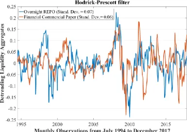
De-trending using Hodrick-Prescott
In order to remove the trend component from the raw data, the Hodrick-Prescott filter is a widely used method to de-trend macro-economic time series, especially GDP aggregates. The filter separates the raw data into a trend component Tt and a cyclical component Ct such that Yt = Tt + Ct.
The minimization problem is: min
𝜏 ∑ 𝐶𝑡
2 𝑇
𝑡=1 + 𝜆 ∑𝑇−1𝑡=2[(𝜏𝑡+1− 𝜏𝑡) − (𝜏𝑡− 𝜏𝑡−1)]2, 𝑤ℎ𝑒𝑟𝑒 𝐶𝑡 = 𝑦𝑡− 𝜏𝑡 (1.10)
The lambda (λ) parameter, which is an adequately chosen positive value, penalizes the effect of the trend component. When λ is increased the trend component will be more penalized. Higher frequency of data requires a higher λ, since short-term fluctuations should not influence the longer term output of the data filtering. Despite there is no consensus between authors on the values of λ to be used, Matlab assumes that for monthly data 14400 is an appropriate value for λ.
In figure 9 are plotted the liquidity aggregates (in Logs), de-trended using this method. The results of the stationarity tests performed on these series point out that de-trending the liquidity aggregates using the Hodrick-Prescott filter produce stationary series. All the unit-root tests strongly reject the null hypothesis that the de-trended data follows a random walk process, with p-values < 0.01. As first-differencing, the HP filter also produces a mean-reverting process, with mean zero. Moreover, the correlation coefficient for the entire sample is 0.28 and 0.50 during the 2007-2008 crisis. The increase in correlation observed during the financial crisis had already been observed in the de-trending of the aggregates with respect to a linear time vector.
Figure 9 - De-trending the Log Repo and the Log Commercial Paper variables using the Hodrick-Prescott filter.
7. Model Specifications
Using simple OLS regressions, three model specifications have been used in order to assess if the good results that are shown in Adrian et al. (2015) still hold with the current data sample. First, only two aggregates were used for the entire sample period (July 1994 until December of 2017), using the three methods of de-trending (linear time trend, first differences and Hodrick-Prescott de-trending). Then it was added a dummy variable to accommodate for possible changes before and after the financial crisis of 2007-2008, and finally, it was used the same crisis dummy with interactions with the liquidity aggregates. The model specifications are the following14:
yt+i= β0 + β1 LogRepot + β2 LogCommercial Papert + et+i (1.11)
yt+1= β0 + β1 LogRepot + β2 LogCommercial Papert + β3DummyCrisist + et+i (1.12)
yt+1= β0 + β1 LogRepot + β2 LogCommercial Papert + β3DummyCrisist + β4DummyCrisist x LogRepot + β5DummyCrisist x LogCommercialPapert + et+i (1.13)
Table 6-a and 6-b shown in the Appendix present the standard t-statistics for the coefficients estimates obtained using (1.11) for the developed countries, as well as F-statistics and the adjusted R-squares. Neither the sign nor the statistical significance of the coefficients is preserved across the three types of de-trending. Although linear time-trend produces more significant estimates for the coefficients, first differencing seems to produce better fitting (the adjusted R-squares are generally higher than those obtained using linear time de-trending at 1 lag and has a similar fit to linear time de-trending at lag 2).
The regressions in which dependent variables are de-trended in respect to linear time and regressed on one-month ahead, currency returns present poor results for the individual significance of the coefficients and for the global significance of the regression. When the lag order of the fitting adjustment is increased for two months, the explanatory power of the regression and the individual significance of the coefficients increase considerably for all cross-rates, except for Japan. The variability in the explanatory power of regressions and coefficient
14 The dependent variable y
t+i is the one-month or the two month currency return (depending on the lag order
significance at different time horizons is well documented in financial literature in (Groen, 1999), (Boudoukh, 2005), (Mark, 1997), and it is mostly attributed to small sample size.
Although the results improve when the lag horizon increases, the adjusted R-squares are lower than those reported on Adrian et al. (2015) at lag 1. More intriguing is that for both forecasting horizons, the sign of the Log Repo is negative for all developed countries and it is statistically significant for eight of the ten developed countries when using linear time de-trending. The negative sign obtained for the Log Repo coefficient goes against the initial hypothesis of studying, that increasing Dollar funding liabilities would lead to a U.S Dollar appreciation. The coefficient for the Log Commercial Paper is also statistically significant for eight of the ten countries and it is significantly positive for seven of the ten countries at lag 2, which goes with the initial claim that increasing Dollar funding liquidity forecasts Dollar appreciations.
Alternatively, when using first differences of liquidity aggregates as regressors in (1.11), the individual significance of the coefficients is lower (the coefficient for the Log Repo is never significant) when compared to linear time de-trending as it has already been said. More unexpected is the negative sign for the coefficient of the Log Commercial Paper. This again goes against the proposed claim, that more Dollar funding liabilities would increase the value of the U.S Dollar against other currencies.
Using the output of the Hodrick Prescott filter as regressors in (1.11) yields very poor results with no single individual coefficient being statistically significant and only two regressions rejecting the null hypothesis of the F-test. Moreover the sign of the coefficients is not consistently positive or negative for the two liquidity aggregates and across the ten countries.
Figure 10 and Figure 11 illustrate the change in the sign of the relationship between the Log Repo and the Log Commercial Paper and the USD/AUD15(U.S Dollar against the
Australian Dollar) across the different de-trending methods. Although the sign of the slope is changing, the slope itself is almost zero. In fact, when currencies are regressed on a single liquidity aggregate (Log Repo or Log Commercial Paper at one lag), the coefficients of these variables are never statistically significant. Therefore it can be concluded that the significance of both liquidity variables (when exists) is due to the interaction between the two variables and not because of each variable’s single effect. It’s hard to compare which de-trending method is
15 Regressing liquidity aggregates on one and two months ahead of USD/AUD currency returns yields the most satisfactory results using linear
time-trend residuals. Therefore the USD/AUD currency returns’ series was chosen to make the argument that the sign of the estimates of the coefficients of liquidity aggregates are changing according with the de-trending method considered.
the best since, although linear de-trending presents best results on the individual statistical significance of coefficients (at two lags) there is some evidence that the series produced by linear time de-trending is not stationary and therefore statistical inference might not be robust. Moreover, the Log Repo coefficient is negative, which does not go along with the initial hypothesis. On the other hand, using First Differences leads to higher R-squares in general but lower significance levels for the individual coefficients of the regressors. Furthermore, the sign of the estimates for the coefficients for both liquidity variables is not consistently the same across countries or across de-trending methods indicating that the effect of the liquidity aggregates on U.S Dollar appreciation/depreciation is not clear. This fact makes harder to draw any economical conclusion.
The maximum adjusted R-square registered for specification (1.11) among the three de-trending methods is 3.71% for the EUR/USD16 cross rate (Table 6b) against 4.00% on the same
16It is not exactly the same currency since the authors use the Deutsche Mark instead of the Euro, but the Deutsche Mark is a widely accepted
proxy for the euro within the academia for periods before 1999.
Figure 10, Figure 11 - Dispersion graph of sample observations of the three de-trending methods used on the Logs of Commercial Paper (left) and on the Logs of Repo (right), regressed on one-month currency returns of the USD/AUD spot exchange rate.
currency pair and 7.10% on the USD/NZD using linear time de-trending as seen in Adrian et al. (2015). The model specification used by the authors has three more variables.
In order to have comparable results, the missing variables will be added in two additional regressions. The authors use a time dummy variable that separates the sample observations in two distinct periods. A period before the 2007-2008 financial crisis and a period after the crisis. The regression in Adrian et al. (2015) also uses the dummy variable with interaction terms with the liquidity variables. This happens because the authors may believe that following the financial crisis of 2008 the effects of the liquidity variables on currency returns have changed. To have closer results to the ones obtained in Adrian et al. (2015), two things must happen with the introduction of these three variables. The additional variables will have to increase the overall explanatory power of the regression, and through their interactions, they will have to change the sign of the Log Repo in the time de-trended regressions and to change the sign of Log Commercial Paper in the first difference de-trending.
Introducing a financial crisis’ dummy in the regression (1.12) to account for the structural change in liquidity markets (Tables 7a, 7b, 7c and 7d) decreases the overall significance of the regression when considering linear time de-trending at lag 1 and increases it for regressions that use linear time de-trending at lag 2 and first differences. Individual significance of the coefficient’s estimates decreases for linear time de-trending and is unchanged for first differences.
For all countries studied (developed and emerging) the coefficient of the dummy variable is never statistically significant as it happens in Table 1 in Adrian et al. (2015), (with exception for two countries). The author’s results present a positive sign for the estimate of the coefficient which means that due to the crisis and considering everything else held at constant levels, the Dollar would be expected to appreciate against the majority of the countries. In the current sample the estimate for the coefficient of the Dummy variable seems to take more positive values for developed countries and more negative values for emerging markets what makes one’s suspect that the Dollar appreciated against currencies from developed countries and depreciated against emerging markets. Figure 1 shows that around 2008 the dollar appreciated against major currencies, and valued and then rapidly devalued against emerging markets.
In model (1.12), although introducing the dummy variable increases the value of the coefficient of the Log Repo as it was expected, for most countries this increase is not enough in magnitude to make the negative coefficients positive and sufficiently positive to make them statistically significant. In fact, lots of coefficients lose negative statistical significance when the dummy is added which in some cases leads to a decrease in the adjusted R-square of the