Todos os direitos reservados.
É proibida a reprodução parcial ou integral do conteúdo
deste documento por qualquer meio de distribuição, digital ou impresso,
sem a expressa autorização do
REAP ou de seu autor.
The Ins and Outs of Unemployment over Different
Time Horizons
Ajax Moreira
Miguel N. Foguel
Carlos Henrique Corseuil
The Ins and Outs of Unemployment over Different Time Horizons
Ajax Moreira
Miguel N. Foguel
Carlos Henrique Corseuil
Ajax Moreira
Instituto de Pesquisa Econômica Aplicada (IPEA)
Miguel N. Foguel
Instituto de Pesquisa Econômica Aplicada (IPEA)
Carlos Henrique Corseuil
The Ins and Outs of Unemployment over Different Time Horizons
Ajax Moreira, Miguel N. Foguel, and Carlos Henrique Corseuil
Abstract: We devise a decomposition for the level of the unemployment rate that allows the assessment of the contributions of the various flow rates in the labor market over different time horizons. The decomposition is sufficiently broad so that the contributions of these factors can be computed for any future period chosen by the analyst. In particular, the decomposition allows one to recover the contributions of the flow rates in the long run as in the steady-state decomposition of Shimer (2012). We apply our methodology for data from the United States and Brazil. The results show that the relative contribution of the flows to the variance of the cyclical component of unemployment is sensitive to the time horizon of the projected unemployment rate. The changes in relative contributions of some flows are so prominent that their rankings change over time.
Keywords: Unemployment, Labor Market Flows, Cyclical Fluctuations, Decomposition.
1. Introduction
Identifying whether the fluctuations in the unemployment rate are due to movements in job
hiring, job separation or the transition between inactivity and unemployment is key to the
understanding of business cycles and the functioning of labor markets. Assessing the relative
importance of these flows also provides valuable information for policymakers to focus on
suitable policies that act on the flows that are more relevant to explaining the movements in
unemployment.
The literature that investigates the relative contributions of worker flows to the cyclicality of
unemployment is extensive.1 The bulk of the literature is based on data for the United States,
and much of the debate evolves around the correct magnitude of the contributions of the inflow
rate to and outflow rate from unemployment in that country. While some studies present
evidence of the dominant role of the fluctuations in the outflow rate (e.g., Hall, 2005; Shimer,
2012), others have found a more balanced role between the two types of flows (e.g., Elsby et
al., 2009; Fujita & Ramey, 2009).
Almost all studies in the recent literature utilize the decomposition method pioneered by Shimer
(2007) in which the relative contributions of the distinct flows are computed under the
assumption that the contemporaneous unemployment rate is very closely approximated by its
Moreira, Foguel, and Corseuil: Instituto de Pesquisa Econômica Aplicada (IPEA). We would like to thank
Maira Albuquerque Penna Franca for preparing the Brazilian data set used in the paper. We are grateful for comments from Gulherme Attuy, André Portela, Eduardo Zylberstajn, and from seminars participants at the Instituto de Pesquisa Econômica Aplicada, Insper, and the 37th Meeting the Brazilian Econometric Society on an earlier version of this paper.
steady-state value.2 Under this assumption, past transitions play no role and the variability of
the current unemployment rate is decomposed only into the contributions of the current flows.
However, using a sample of 14 OECD countries, Elsby et al. (2013) show that the use of the
steady-state rate as a proxy for the observed rate is accurate for the United States but not for
other developed countries, in particular those in continental Europe.3 By extending the
decomposition method devised by Elsby et al. (2009) for changes in the current unemployment
rate, Elsby et al. (2013) show that when unemployment deviates from the steady state, past and
current flow rates matter for the variation in the current unemployment rate. These results
evince that the use of decompositions based on steady-state unemployment provide a good
approximation for countries with fast labor market dynamics – such as the United States – where
the current unemployment rate quickly adjusts to its steady-state value after the occurrence of
shocks. For countries with slower dynamics, one should rely on decomposition methods that
provide accurate answers, even when unemployment is out of the steady state.
In this paper, we devise a decomposition for the level of the unemployment rate that can be
used for countries with different labor market dynamics. The decomposition is based on
projections of the unemployment rate for different time horizons as alternative proxies for the
current rate. These projections are computed as the rate that would prevail in a future period
when one uses the information available in the current period on the initial conditions – which
are captured by the lagged unemployment rate – and the flow rates. As it spawns a sequence of
projections of the unemployment rate over time, our proposed decomposition is sufficiently
broad to allow for the assessment of the contributions of these factors for any future period
chosen by the analyst. At the one extreme, if interest lies in the very short term, the
decomposition informs the contributions of these factors for the projection of the
unemployment rate of just one period ahead of the current period. This approach is what we
shall call the short-term decomposition. At the other extreme, if one is interested in the distant
future, the decomposition allows one to recover the contributions of the flow rates as in the
steady-state decomposition of Shimer (2012). In our empirical analysis, we not only contrast the
decomposition results for these two extreme cases but also exploit the wealth of results that fall
in between them.
2 Shimer (2007) was eventually published in 2012, but the 2007 version had a great influence on the papers published before 2012.
It should be pointed out that, similar to Shimer (2012), our decomposition provides information
on the determinants of the level of the unemployment rate. This feature contrasts with the
decompositions used by Elsby et al. (2009), Fujita and Ramey (2009), and Eslby et al. (2013), all
of which address (log) changes in the unemployment rate. While these decompositions are
interesting in their own right, they address a different object from ours.
We apply our decomposition for data from the United States and Brazil. For the former country,
we use gross flow data from the Current Population Survey (CPS) over the 1990-2015 period.
For the latter, we compute the gross flows from the Pesquisa Mensal de Emprego (PME, Monthly
Employment Survey), which is a household survey with a very similar sampling design as that of
the CPS, that was conducted by the Instituto Brasileiro de Geografia e Estatística (IBGE, the
Brazilian Bureau of Census) in the six major Brazilian metropolitan areas over the period
2002-2016. Following the literature, we apply standard filters to the data for the two countries to
adjust for seasonality, trends, and time aggregation bias.
We present the results for both countries using our decomposition method and the steady-state
decomposition of Shimer (2012). The results show that the relative contribution of the flows to
the variance of the cyclical component of unemployment is sensitive to the time horizon of the
projected unemployment rate. For some flows, the changes in relative contributions are so
prominent that their rankings change towards the path to the steady state. These qualitative
changes are more substantial for the case of Brazil. Though the relevance of initial conditions is
quite significant in the short run for both countries, they quickly lose importance over longer
time horizons. The results also show that the steady state rate of unemployment is not a very
good proxy for the current rate in Brazil. This suggests that the projected unemployment rate
over shorter time horizons should be considered as an alternative to the steady state
approximation in countries where the latter performs poorly as a proxy for current
unemployment.
The article proceeds as follows. Section 2 presents the basic framework and our decomposition
method. Different from the literature, the presentation uses matrix notation, which is more
compact and allows the analyst to address as many labor market states as desired. Section 3
describes the data for the United States and Brazil and presents the evolution of the current and
the steady-state unemployment rates for both countries. Section 4 contains the results from our
decomposition for the short and the long term and for the periods in between them. In Section
2. Methodology
Considering a labor market with 𝑆 possible states (e.g., employment, unemployment, and
inactivity), the basic structure of the transition model consists of two components, a state
probability vector, 𝑝𝑡 = (𝑝1𝑡, … , 𝑝𝑆𝑡)′, and a 𝑆 × 𝑆 transition matrix, 𝜋𝑡, whose columns add up
to one and in which a typical element 𝜋𝑡(𝑖, 𝑗) represents the probability of transitioning from
state i to state 𝑗 from period 𝑡 − 1 to period 𝑡. Assuming a population of working age that is
constant over time, the transition matrix 𝜋𝑡 relates the vectors 𝑝𝑡 and 𝑝𝑡−1 in a Markovian sense
as follows:4
𝑝𝑡 = 𝜋𝑡𝑝𝑡−1. (1)
The current unemployment rate, 𝑢𝑡, can be computed from the probability vector 𝑝𝑡 and thus
can be expressed as a function of 𝜋𝑡 and 𝑝𝑡−1. Specifically, denoting the probabilities of being
employed and unemployed respectively by 𝑝𝑒𝑡and 𝑝𝑢𝑡, the unemployment rate can be
expressed as follows:
𝑢𝑡 =𝑝𝑒𝑡𝑝+𝑝𝑢𝑡𝑢𝑡= 𝑢(𝜋𝑡𝑝𝑡−1), (2)
where 𝑢(. ) is a function that transforms the product of the transition matrix and the state
probabilities in the previous period into the current rate of unemployment.
The decomposition methodology proposed by Shimer (2012) uses the concept of the
steady-state probability, 𝑝𝑡∗, which is calculated under the assumption that for each period 𝑡 the
transition matrix 𝜋𝑡 is constant in subsequent periods and that the state probability for ℎ periods
ahead, 𝑝𝑡+ℎ, converges to 𝑝𝑡∗ when ℎ grows to infinity. Assuming convergence, 𝑝𝑡∗ can be
calculated by solving the following system:
𝑝𝑡∗= 𝜋𝑡𝑝𝑡∗= 𝐹(𝜋𝑡), (3)
where 𝐹(. ) is a matrix function whose arguments are the elements of 𝜋𝑡. The rate at which the
system converges to 𝑝𝑡∗ depends on certain properties of the transition matrix. When
convergence is sufficiently rapid, the vector 𝑝𝑡∗ provides a good approximation to 𝑝𝑡 and the
current unemployment rate, 𝑢𝑡, can be well approximated by the long-term rate of
unemployment, 𝑢𝑡∗= 𝑢(𝑝𝑡∗) = 𝑢(𝐹(𝜋𝑡)). Shimer (2012) reports that the correlation between
the steady state’s and the next month’s unemployment rate is 0.99 for the United States. Based
on this result, he claims that the steady state rate is a good measure to apply in his
decomposition method.
However, as argued by Elsby et al. (2013), while the decomposition based on the steady state
rate may be reasonably accurate for the United States – a country known to have a flexible labor
market – it may not provide an accurate description of the fluctuations in the current rate for
countries that display slower unemployment dynamics. This point raised by Elsby et al. (2013)
inspired us to devise a decomposition method for contexts in which the level of the
unemployment rate is out of the steady state.
In what follows, we present two decomposition methods of the unemployment rate: the
long-term, steady-state version proposed by Shimer (2012) and ours, which we call the
decomposition on the projected unemployment rate. The two decompositions follow the
approach for the nonlinear factoring of systems used by Shimer (2012) and are detailed in the
following two sections. To show the operation of these decompositions, we shall detail them
initially for a two-state labor market, in which the model is simpler, and subsequently for a
market with any number of states.
2.1. Decomposition of the Unemployment Rate with Two Labor Market States
In the context of a labor market with only two states (employed, 𝑒, and unemployed, 𝑢), it is
assumed that the labor force (𝑙 = 𝑒 + 𝑢) remains constant over time. The transition matrix 𝜋𝑡
is a square 2 × 2 matrix, where the elements in the main diagonal represent the probability of
remaining in the respective state and the off-diagonal elements represent the probability of
transition between the two states between months 𝑡 − 1 and 𝑡. In this context, expression (1)
is written as follows:
[𝑝𝑝𝑒𝑡 𝑢𝑡] = [𝜋
𝑡(𝑒, 𝑒) 𝜋𝑡(𝑢, 𝑒) 𝜋𝑡(𝑒, 𝑢) 𝜋𝑡(𝑢, 𝑢)] [
𝑝𝑒𝑡−1
𝑝𝑢𝑡−1] = [1 − 𝑠
𝑡 𝑓𝑡
𝑠𝑡 1 − 𝑓𝑡] [ 𝑝𝑒𝑡−1 𝑝𝑢𝑡−1],
where 𝑓𝑡denotes the probability of transition from unemployment to employment – the
outflow rate – and 𝑠𝑡 denotes the probability of transition from employment to unemployment
– the inflow rate.
Assuming that the labor force remains constant between adjacent months, the current
unemployment rate can be expressed as follows:
𝑢𝑡 = 𝑝𝑢𝑡= 𝑠𝑡𝑝𝑒𝑡−1+ [1 − 𝑓𝑡]𝑝𝑢𝑡−1= 𝑠𝑡(1 − 𝑢𝑡−1) + [1 − 𝑓𝑡]𝑢𝑡−1 = 𝑢𝑡−1𝜆𝑡+𝑠𝑡, (4)
Given the information available in 𝑡, the projected unemployment rate for period 𝑡 + ℎ can be
obtained recursively from (4) as follows:
𝑢𝑡+ℎ = 𝑢𝑡−1𝜆ℎ+1𝑡 +𝑠𝑡(1 + ⋯ + 𝜆𝑡ℎ), ∀ℎ = 0,1,2, … (5)
Assuming (𝑠𝑡+ 𝑓𝑡) < 1, 𝜆𝑡 in expression (5) measures the rate of convergence of the projected
unemployment rate to the long-term rate. The long-term rate can be calculated by assuming
that unemployment is in steady state (i.e., 𝑢𝑡 = 𝑢𝑡−1= 𝑢𝑡∗) or extrapolating the time horizon to
infinity:
𝑢𝑡∗= 𝐺(𝑠𝑡, 𝑓𝑡) =𝑠𝑡𝑠+𝑓𝑡𝑡= limℎ→∞𝑢𝑡+ℎ = limℎ→∞[𝑢𝑡−1𝜆𝑡ℎ+1+𝑠𝑡(1 + ⋯ + 𝜆𝑡ℎ)], (6)
where we used expression (5) in the last equality.
In summation, for each period 𝑡, expression (4) determines the current unemployment rate, 𝑢𝑡,
and expression (5) represents a sequence of projected unemployment rates, 𝑢𝑡+ℎ, ℎ = 0,1,2, …,
which connects to the long-term unemployment rate through equation (6) when ℎ goes to
infinity. Equation (6) makes explicit the connection between the projected and the long-run
rates and shows the role played by the rate of convergence 𝜆𝑡 in the relationship between these
rates, namely, the smaller the value of 𝜆𝑡– that is, the higher the inflow rate (𝑠𝑡) and the outflow
rate (𝑓𝑡) – the faster the convergence to the long-term unemployment rate, 𝑢𝑡∗.
The long-term unemployment rate, 𝑢𝑡∗, is the object of the decomposition proposed by Shimer
(2012), which is given by the following linear approximation:5
𝑢𝑡∗≅𝑠̅+𝑓̅𝑠̅ + {𝑠𝑡𝑠+𝑓̅𝑡 −𝑠̅+𝑓̅𝑠̅ } + {𝑠̅+𝑓𝑠̅𝑡−𝑠̅+𝑓̅𝑠̅ } = 𝑘∗+ [𝑢𝑠(𝑠𝑡) − 𝑘∗] + [𝑢𝑓(𝑓𝑡) − 𝑘∗] = 𝑘∗+ 𝑢𝑠𝑡+ 𝑢𝑓𝑡, (7)
where 𝑘∗= 𝑠̅
𝑠̅+𝑓̅ and 𝑠̅ and 𝑓̅ represent the average inflow and outflow rates over sample period,
respectively. Note that only 𝑠𝑡 or 𝑓𝑡 is permitted to vary at a time and sum of the terms 𝑢𝑠𝑡 and
𝑢𝑓𝑡 only capture the approximate contributions of the inflow and outflow rates to the deviation
of steady-state unemployment rate.
5 𝑢
𝑡
∗= 𝐺(𝑠
𝑡, 𝑓𝑡) ≅ 𝐺(𝑠̅, 𝑓̅) +𝜕𝐺(𝑠̅,𝑓̅)𝜕𝑠𝑡 (𝑠𝑡− 𝑠̅) +𝜕𝐺(𝑠̅,𝑓̅)𝜕𝑓𝑡 (𝑓𝑡− 𝑓̅) ≅ 𝐺(𝑠̅, 𝑓̅) +[𝐺(𝑠𝑡,𝑓̅)−𝐺(𝑠̅,𝑓̅)](𝑠𝑡−𝑠̅) (𝑠𝑡− 𝑠̅) + [𝐺(𝑠̅,𝑓𝑡)−𝐺(𝑠̅,𝑓̅)]
(𝑓𝑡−𝑓̅) (𝑓𝑡− 𝑓̅) = 𝐺(𝑠̅, 𝑓̅) + [𝐺(𝑠𝑡, 𝑓̅) − 𝐺(𝑠̅, 𝑓̅)] + [𝐺(𝑠̅, 𝑓𝑡) − 𝐺(𝑠̅, 𝑓̅)]. Replacing G(.) in this
The decomposition we propose is also based on the same idea of varying the elements that
comprise the current unemployment rate, one at a time. Based on analogous linear
approximation applied to expression (4), the decomposition can then be expressed as follows:
𝑢𝑡 ≅ 𝑘 + {𝑢𝑡−1[1 − 𝑠̅ − 𝑓̅] + 𝑠̅ − 𝑘} + {𝑢̅[1 − 𝑠𝑡− 𝑓̅] + 𝑠𝑡− 𝑘} + {𝑢̅[1 − 𝑠̅ − 𝑓𝑡] + 𝑠̅ − 𝑘} = 𝑘 + [𝑣0(𝑢𝑡−1) − 𝑘] + [𝑣𝑠(𝑠𝑡) − 𝑘] + [𝑣𝑓(𝑓𝑡) − 𝑘] = 𝑘 + 𝑣0𝑡+ 𝑣𝑠𝑡+ 𝑣𝑓𝑡 (8)
where 𝑘 = {𝑢̅[1 − 𝑠̅ − 𝑓̅] + 𝑠̅}, 𝑢̅ represents the average unemployment rate over the sample
period, 𝑣0𝑡 captures the contribution of lagged unemployment, and 𝑣𝑠𝑡 and 𝑣𝑓𝑡 represent
respectively the contributions of the inflow and outflow rates on the deviation of
contemporaneous unemployment rate.
The projected unemployment rate described in (5) can also be decomposed into analogous main
components 𝑣0𝑡+ℎ, 𝑣𝑠𝑡+ℎ, and 𝑣𝑓𝑡+ℎ, obtaining the following expression:
𝑢𝑡+ℎ ≅ 𝑣0𝑡+ℎ+ 𝑣𝑠𝑡+ℎ+ 𝑣𝑓𝑡+ℎ, ∀ℎ = 0,1,2, … . (9)
If expressions (7) and (9) constitute good approximations respectively to the long-term and
projected unemployment rates, then the variances of these rates can be approximated as
follows:
𝑉(𝑢𝑡∗) ≅ 𝑐𝑜𝑣〈𝑢𝑡∗, 𝑢𝑠𝑡〉 + 𝑐𝑜𝑣〈𝑢𝑡∗, 𝑢𝑓𝑡〉 (10)
and
𝑉(𝑢𝑡+ℎ) ≅ 𝑐𝑜𝑣〈𝑢𝑡+ℎ, 𝑣0𝑡+ℎ〉 + 𝑐𝑜𝑣〈𝑢𝑡+ℎ, 𝑣𝑠𝑡+ℎ〉 + 𝑐𝑜𝑣〈𝑢𝑡+ℎ, 𝑣𝑓𝑡+ℎ〉. (11)
If we divide both sides of (10) and (11) by their respective variances, we then obtain a method
of computing the approximate contributions of the components of each expression to the
fluctuations in the unemployment rate of interest. More specifically,
𝑉(𝑢𝑡∗)
𝑉(𝑢𝑡∗)= 1 ≅𝑐𝑜𝑣〈𝑢𝑡 ∗,𝑢𝑠𝑡〉
𝑉(𝑢𝑡∗) +𝑐𝑜𝑣〈𝑢𝑡 ∗,𝑢𝑓𝑡〉
𝑉(𝑢𝑡∗) = 𝛽𝑠∗+ 𝛽𝑓∗ (12)
where the 𝛽s measure the contributions of the components that appear in their respective
subscripts in each expression. And
𝑉(𝑢𝑡+ℎ)
𝑉(𝑢𝑡+ℎ)= 1 ≅
𝑐𝑜𝑣〈𝑢𝑡+ℎ,𝑣0𝑡+ℎ〉
𝑉(𝑢𝑡+ℎ) +
𝑐𝑜𝑣〈𝑢𝑡+ℎ,𝑣𝑠𝑡+ℎ〉
𝑉(𝑢𝑡+ℎ) +
𝑐𝑜𝑣〈𝑢𝑡+ℎ,𝑣𝑓𝑡+ℎ〉
𝑉(𝑢𝑡+ℎ) = 𝛽0
ℎ+ 𝛽
𝑠ℎ+ 𝛽𝑓ℎ, (13)
It can be shown that as ℎ grows, 𝑣0𝑡+ℎ converges to zero and 𝑣𝑠𝑡+ℎ and 𝑣𝑓𝑡+ℎ converge to their
corresponding elements of the long-term decomposition in (7) (respectively, 𝑢𝑠𝑡and 𝑢𝑓𝑡).6 As a
consequence, given the relations stated in expressions (12) and (13), 𝛽0ℎ will converge to zero
and 𝛽𝑠ℎ and𝛽𝑓ℎ will converge respectively to 𝛽𝑠∗ and𝛽𝑓∗.
One direct method of calculating these 𝛽s and their respective standard errors is by means of
linear regressions, where each component is regressed against the unemployment rate to which
it is associated. Specifically, to estimate the 𝛽s in the case of (12),
𝑢𝑚𝑡 = 𝛼𝑚∗ + 𝛽𝑚∗𝑢𝑡∗+ 𝜖𝑚𝑡∗ , (14)
where 𝑚 = 𝑠, 𝑓. The coefficients of the decomposition of the short-term unemployment rate
are obtained in the same fashion:
𝑣𝑚𝑡+ℎ= 𝛼𝑚ℎ + 𝛽𝑚ℎ𝑢𝑡+ℎ+ 𝜖𝑚𝑡+ℎ, (15)
where 𝑚 = 0, 𝑠, 𝑓 and ℎ = 0,1,2, ….
It is worth noting that if (7) or (9) is a good approximation of their corresponding unemployment
rates, then (𝛽𝑠∗+ 𝛽𝑓∗) or (𝛽0ℎ+ 𝛽𝑠ℎ+ 𝛽𝑓ℎ) will be approximately equal to one.
2.2. Decomposition of the Unemployment Rate with More Than Two Labor Market States
The results of the previous section may be expanded to systems with larger numbers of states.
We are interested here in the case of three states, which incorporates into the two-state setting
the transitions between the state of inactivity (i.e., out of the labor force) to and from the states
of employment and unemployment.7
Assuming that the transition matrix is constant within a forecasting horizon, one can use
expression (1) recursively to obtain the forecasts for horizon ℎ. The transition matrix 𝜋𝑡 can be
decomposed into its eigenvectors γ𝑡 and eigenvalues Λ𝑡 such that 𝜋𝑡 = 𝛾𝑡Λ𝑡γ𝑡−1, where Λ𝑡 is
the rate of convergence of the matrix in period 𝑡. We can then write the following for period
𝑡 + ℎ:
𝑝𝑡+ℎ = 𝜋𝑡ℎ+1𝑝𝑡−1 = (𝛾𝑡Λ𝑡ℎ+1γ𝑡−1)𝑝𝑡−1, ∀ℎ = 0,1,2, …. (16)
The empirical results of this decomposition show that the characteristic roots are always real,
nonnegative, and not greater than one, which ensures that the sequence Λ𝑡ℎ+1, ℎ + 1 = 1,2, …
converges to a constant matrix. The vector 𝑝𝑡∗ can be obtained either from the function 𝐹(. ) in
expression (3) or from extrapolating the time horizon to infinity:
𝑝𝑡∗= 𝐹(𝜋𝑡) = 𝑙𝑖𝑚ℎ→∞𝑝𝑡+ℎ= 𝑙𝑖𝑚ℎ→∞𝜋𝑡ℎ+1𝑝𝑡−1, (17)
where in the last equality we used expression (16).
The steady-state unemployment rate 𝑢𝑡∗= 𝑢[𝐹(𝜋𝑡)] and the projected unemployment rate
𝑢𝑡+ℎ = 𝑢(𝜋𝑡ℎ+1𝑝𝑡−1), ∀ℎ = 0,1,2, …, where 𝑢(. ) is the function introduced in expression (2),
can be decomposed using linear approximations into factors that represent each (linearly
independent) component of the transition matrix and, additionally, into the factor that
represents the lagged unemployment (except for the long-term unemployment decomposition).
To express these decompositions, let 𝜋̅ be the average of the transition matrices over the sample
period. For each component 𝑖𝑗, we define the transition matrix 𝜓(𝜋𝑡(𝑖, 𝑗); 𝜋̅) = 𝜓𝑡𝑖,𝑗, where all
elements of the matrix are equal to their corresponding elements in 𝜋̅ except the element
𝜋𝑡(𝑖, 𝑗) and those belonging to the main diagonal, which are adjusted to add up to one in the
corresponding column. Formally, denoting any element of 𝜓𝑡𝑖,𝑗 as 𝑎𝑡𝐼,𝐽, this matrix can be written
for the transition from 𝑖 to 𝑗, as follows:8
𝜓(𝜋𝑡(𝑖, 𝑗); 𝜋̅) = 𝜓𝑡𝑖,𝑗= {
𝑎𝑡𝐼,𝐽= 𝜋𝑡(𝑖, 𝑗) 𝑖𝑓 𝐼 = 𝑖, 𝐽 = 𝑗 𝑎𝑡𝐼,𝐽= 1 − ∑𝐼≠𝐽𝑎𝑡𝐼,𝐽𝑖𝑓 𝐼 = 𝐽 𝑎𝑡𝐼,𝐽 = 𝜋̅(𝑖, 𝑗) 𝑜𝑡ℎ𝑒𝑟𝑤𝑖𝑠𝑒.
(18)
This family of transition matrices is used to isolate the contribution of each transition between
the states (𝑖, 𝑗), 𝑖𝑗 in explaining the fluctuations in the unemployment rate.
Similar to that in the two-state context, the decomposition of the long-term unemployment rate
here follows the same approach proposed by Shimer (2012): the contribution of each transition
from 𝑖 to 𝑗, 𝑖𝑗, are added together, where each component of the decomposition captures only
8 For example, in the three-state model with (𝑖, 𝑗) = (2,3), 𝜓
𝑡2,3 is the following matrix:
𝜓(𝜋𝑡(2,3); 𝜋̅) = 𝜓𝑡2,3= [
1 − 𝜋̅(2,1) − 𝜋̅(3,1) 𝜋̅(2,1) 𝜋̅(3,1)
𝜋̅(1,2) 1 − 𝜋̅(1,2)
𝜋̅(3,2) − 𝜋̅(3,2)
𝜋̅(1,3) 𝜋𝑡(2,3) 1 − 𝜋𝑡(2,3) − 𝜋̅(1,3)
the variation in 𝜋𝑡(𝑖, 𝑗). Specifically, using the matrix 𝜓(𝜋𝑡(𝑖, 𝑗); 𝜋̅) defined in (18), the
decomposition of the long-term unemployment rate can be expressed as follows:
𝑢𝑡∗= 𝑢[𝐹(𝜋𝑡)] ≅ 𝜅∗+ ∑ {𝑢(𝐹(𝜓(𝜋𝑖≠𝑗 𝑡(𝑖, 𝑗); 𝜋̅))) − 𝜅∗}= 𝜅∗+ ∑ 𝑢𝑖≠𝑗 𝑖𝑗𝑡∗ , (19)
where 𝜅∗= 𝑢[𝐹(𝜋̅)].
Similarly, the decomposition of the projected unemployment rate is given by the following:
𝑢𝑡+ℎ = 𝑢(𝜋𝑡ℎ+1𝑝𝑡−1) ≅ 𝜅ℎ+ [𝑢(𝜋̅ℎ+1𝑝𝑡−1) − 𝜅ℎ] + ∑ {𝑢𝑖≠𝑗 (𝜓ℎ+1(𝜋𝑡(𝑖, 𝑗); 𝜋̅)𝑝̅) − 𝜅ℎ} = 𝜅ℎ+ 𝑢0𝑡+ℎ+ ∑ 𝑢𝑖≠𝑗 𝑖𝑗𝑡ℎ , ∀ℎ = 0,1,2, …., (20)
where 𝜅ℎ= 𝑢(𝜋̅𝑡ℎ+1𝑝̅).
Analogous to the two-state context, the contribution of each component of the long-term
unemployment rate, 𝑢𝑡∗, in equation (19) and of the predicted unemployment rate, 𝑢𝑡+ℎ, in
equation (20) may be obtained by regressing the time series of each (time-varying) component
against the time series of the projected unemployment rate to which they are associated. In the
case of the long-term rate, the regression is as follows:
𝑢𝑖𝑗𝑡∗ = 𝛼
𝑖𝑗∗ + 𝛽𝑖𝑗∗𝑢𝑡∗+ 𝜖𝑖𝑗𝑡∗ , 𝑖𝑗, (21)
where 𝛽𝑖𝑗∗ captures the contribution of the transition from state 𝑖 to a different state 𝑗.
In the case of the projected unemployment rate, we have the following:
𝑢0𝑡+ℎ= 𝛼0ℎ+ 𝛽0ℎ𝑢𝑡+ℎ+ 𝜖𝑖𝑗𝑡+ℎ, ℎ = 0,1, …. (22’)
𝑢𝑖𝑗𝑡+ℎ= 𝛼𝑖𝑗ℎ + 𝛽𝑖𝑗ℎ𝑢𝑡+ℎ+ 𝜖𝑖𝑗𝑡+ℎ, 𝑖𝑗, ℎ = 0,1, …., (22’’)
where 𝛽0ℎcaptures the contributions of lagged labor market conditions and 𝛽𝑖𝑗ℎthe contribution
of the transition between state 𝑖 to state 𝑗 ≠ 𝑖.
In the appendix, we show that as ℎ grows, the term 𝑢0𝑡ℎ converges to zero and 𝑢𝑖𝑗𝑡+ℎ converge
to their respective long-term decomposition factors 𝑢𝑖𝑗𝑡∗ . As before, this suffices for 𝛽0ℎ to
converge to zero and 𝛽𝑖𝑗ℎ to 𝛽𝑖𝑗∗.
As already stated, if the decomposition based on the projected unemployment rate fully
captures the fluctuations in the observed rate, then 𝛽0ℎ+ ∑ 𝛽𝑖≠𝑗 𝑖𝑗ℎ should be approximately
3. Data and Empirical Preliminaries
The empirical results of the decomposition methods described in the previous section were
obtained for the United States and Brazil. For the former country, we use the monthly gross flow
data from the Current Population Survey (CPS) released by the Bureau of Labor Statistics for the
period from January 1990 to December 2015. For the latter country, we compute monthly gross
flows from the Pesquisa Mensal de Emprego (PME, Monthly Employment Survey), which was
conducted by the Instituto Brasileiro de Geografia e Estatística (IBGE, the Brazilian Census
Bureau) in the six major metropolitan areas in the country and whose sampling design is very
similar to that of the CPS.9
The monthly gross flow data for each country were subjected to the following filters. First, the
monthly series were seasonally adjusted using the US Census Bureau's X12 software. Second,
we use the methodology put forward by Shimer (2012) to adjust for intra-month aggregation
bias and then take the quarterly averages of the resulting monthly series. The last step was to
detrend the quarterly data through the HP filter with the same smoothing parameter used by
Shimer (2012), 105. The resulting filtered transition matrices were then finally subjected to the
methodology described in the previous section to decompose the fluctuations of the short- and
long-term unemployment rates.10
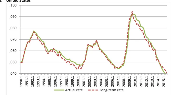
Figures 1a and 1b present the actual and the long-term unemployment rates for the United
States and Brazil, respectively. As it has been shown in the literature (e.g., Shimer, 2012; Elsby
et al., 2013), the actual rate is very closely approximated by the long-term rate for the United
States. However, this is not the case for Brazil, where the observed rate deviates a great deal
from the long-run rate throughout the sample period. Thus, similar to the evidence presented
for other countries in Elsby et al. (2013), the steady-state rate of unemployment is not a good
proxy for the current rate in Brazil either. It is interesting to note, however, that the large gap
between the actual and the long-term rates for Brazil becomes considerably lower when shorter
horizons are considered. This is can be seen from the comparison between the actual and the
short-term rate in Figure 1b.
9 The six metropolitan areas are as follows: Porto Alegre, São Paulo, Rio de Janeiro, Belo Horizonte, Salvador, and Recife. Around 40% of the Brazilian population live in those areas. As in the CPS, the PME follows a 4-8-4 rotation scheme so that households are surveyed for four consecutive months, leave the sample for eight months, and are interviewed again for four additional months.
Figure 1: Observed and long-term unemployment rates
a. United States
b. Brazil
Note: The actual unemployment rate is computed from expression (2) [𝑢𝑡= 𝑢(𝜋𝑡𝑝𝑡−1)] and the long-term rate from expression (3) using 𝑢𝑡∗= 𝑢(𝐹(𝜋𝑡)). The rates are based on data for the three-state context. ,040 ,050 ,060 ,070 ,080 ,090 ,100 19 90.1 19 91.1 19 92.1 19 93.1 19 94.1 19 95.1 19 96.1 19 97.1 19 98.1 19 99.1 20 00.1 20 01.1 20 02.1 20 03.1 20 04.1 20 05.1 20 06.1 20 07.1 20 08.1 20 09.1 20 10.1 20 11.1 20 12.1 20 13.1 20 14.1 20 15.1
Actual rate Long-term rate
0,060 0,070 0,080 0,090 0,100 0,110 0,120 0,130 1990.1 19 90 .3
1991.1 1991.3 1992.1 1992.3 1993.1 1993.3 1994.1 1994.3 1995.1 1995.3 1996.1 1996.3 1997.1 1997.3 19
98
.1
1998.3 1999.1 1999.3 2000.1 2000.3 2001.1 2001.3 2002.1 2002.3
4. Decomposition Results
4.1 Results for the Long- and Short-Term Decompositions
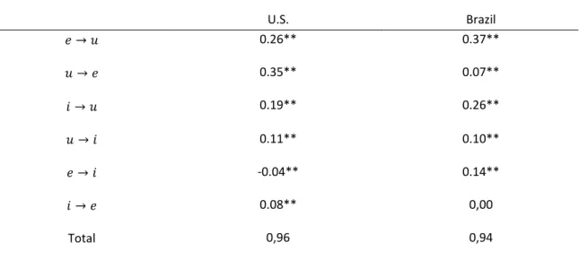
Table 1 presents the results from the long-term decomposition in the three-state context for
Brazil and the United States. The first two columns report the estimates of the 𝛽s based on
equation (21). The contributions of the transition rates are displayed in the rows. The results for
the United States are qualitatively similar to those of Shimer (2012). The most important
transition is the outflow from unemployment into employment (ue), which is followed by the
reverse transition (eu) and the flow from inactivity into unemployment (iu). Compared to those
of the United States, the main differences for the case of Brazil are the much lesser role played
by the exit from unemployment into employment (ue) and the higher importance of the
transitions from employment and inactivity into unemployment (eu and iu).11
Table 1: Decomposition of the long-term unemployment rate in the three-state context
U.S. Brazil
𝑒 → 𝑢 0.26** 0.37**
𝑢 → 𝑒 0.35** 0.07**
𝑖 → 𝑢 0.19** 0.26**
𝑢 → 𝑖 0.11** 0.10**
𝑒 → 𝑖 -0.04** 0.14**
𝑖 → 𝑒 0.08** 0,00
Total 0,96 0,94
Note: See the text for the decomposition methodology and measurement issues. The coefficients are presented along with their statistical significance according to the notation: p-value: < 0.05 (**), and <
0.1 (*). Key: Transitions are defined between the inactive (i), unemployed (u), and employed (e) states.
The last row of Table 1 shows the sum of the contributions. As previously pointed out, if the
steady-state unemployment rate is a good approximation for the actual rate, then the sum of
the contributions should be close to 1. However, as it can be seen, the results do not appear to
confirm that this is the case, especially for Brazil, for which the sum of the contributions falls
short by 0.06 points. This result reinforce what was displayed in Figure 1, which also shows that
the steady state approximation was relatively worse for Brazil. As pointed out by Elsby et al.
(2013), the presence of large approximation errors calls into question the use of the steady-state
decomposition to gauge the contributions of the flows rates to cyclical movements in the
unemployment rate.
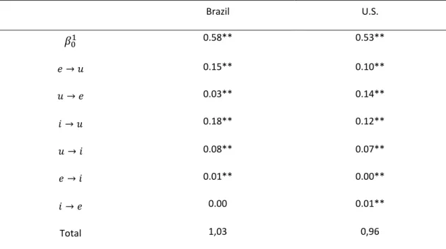
Table 2: Decomposition of the short-term unemployment rate in the three-state context
Brazil U.S.
𝛽01 0.58** 0.53**
𝑒 → 𝑢 0.15** 0.10**
𝑢 → 𝑒 0.03** 0.14**
𝑖 → 𝑢 0.18** 0.12**
𝑢 → 𝑖 0.08** 0.07**
𝑒 → 𝑖 0.01** 0.00**
𝑖 → 𝑒 0.00 0.01**
Total 1,03 0,96
Note: See the text for the decomposition methodology and measurement issues. 𝛽01 refers to the contribution of the initial conditions. The coefficients are presented along with their statistical significance according to the notation: p-value: < 0.05 (**), and < 0.1 (*). Key: Transitions are defined between the inactive (i), unemployed (u), and employed (e) states.
Table 2 reports the results from our proposed decomposition of the short-term unemployment
rate of equations (22’) and (22’’) (using the projected unemployment rate when ℎ = 1). Compared to the layout of Table 1, the only new element in Table 2 is in the first row, which
contains the estimated contribution of the lagged conditions (i.e., 𝛽01in equation (22’)). There
are some notable results in Table 2. First, the sum of the contributions is now closer to 1 for
Brazil. This result reveals that by taking into account the influence of the lagged conditions, the
short-term decomposition can mitigate the approximation errors that turn up in the
steady-state decomposition. Second, compared to the long-term decomposition, there are important
changes in the relative contributions of the flows in the short-run decomposition for both the
United States and Brazil. In particular, ranks flip for the components of the inflows into
unemployment (eu and iu). In the short-run decomposition, the inflow to unemployment from
inactivity (iu) became more important than the inflow to unemployment from employment (eu)
in both countries. Another notable change in rank refers to the flow from employment to
inactivity (ei) for Brazil. This flow was the third most important to explain the variance of
steady-state unemployment. But its contribution became negligible when the decomposition is
Table 2 shows, the previous state of the labor market explains more than 50% of the cyclical
fluctuations in the short-run rate in each country. This result reveals that the lagged conditions
and, therefore, the past transitions across the states do matter to explaining the cyclicality of
the short-term unemployment rate.
4.2.Connection of the short-term to the long-term decomposition
As presented in equation (20), the decomposition on the projected unemployment rate allows
the computation of the contributions of the initial conditions and the current transition rates for
periods ℎ = 1,2, … ahead of the reference period 𝑡. To compute the contributions of these
components over time, we estimate equations (22’) and (22’’) to obtain a sequence of 𝛽0ℎ and
𝛽𝑖𝑗ℎ, ∀𝑖 ≠ 𝑗, for different time horizons. As discussed in section 2, as ℎ grows unbounded, we
should expect 𝛽0ℎ to converge to zero and 𝛽𝑖𝑗ℎ, ∀𝑖 ≠ 𝑗, to converge to their long-term
counterparts in the steady-state decomposition.
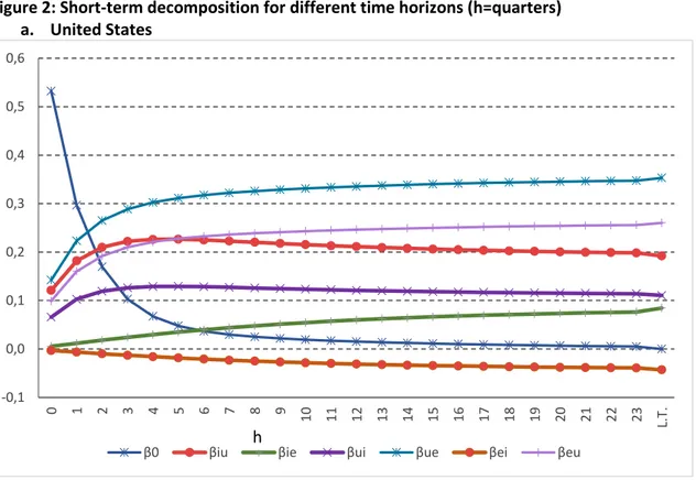
Figures 2a and 2b show the estimated 𝛽0ℎ and 𝛽𝑖𝑗ℎ for each transition 𝑖 ≠ 𝑗 for ℎ = 1,2, … ,24
quarters for the United States and Brazil, respectively. The final point on the lines for the 𝛽𝑖𝑗ℎ
reports the corresponding 𝛽𝑖𝑗∗ estimated from the steady-state decomposition.
Figure 2: Short-term decomposition for different time horizons (h=quarters) a. United States
-0,1 0,0 0,1 0,2 0,3 0,4 0,5 0,6
0 1 2 3 4 5 6 7 8 9
10 11 12 13 14 15 16 17 18 19 20 21 22 23 L.T.
b. Brazil
Note: The βs corresponds to the contributions of the transition rates to the variance of the cyclical component of the projected unemployment rates. The L.T. in the horizontal axis refers to long-term and displays the decomposition results from the steady-state decomposition.
Some results in Figures 2a and 2b are noteworthy. First, the Figures show that the influence of
the initial state of the labor market converges to zero as ℎ grows and that all the contributions
of the transition rates of the short-term decomposition tend to converge to their analogues in
the long-term decomposition. Second, the contribution of the initial conditions quickly
decreases for both countries, beginning at above 50% in the first period (ℎ = 1) and reaching
values of approximately 10% in the fourth quarter (ℎ = 4). This result shows that the initial state
of the labor market is highly relevant in the short run but quickly loses its influence in explaining
the dynamics of unemployment.
The evolution of the relative importance of each flow according to the time horizon of the
projected unemployment rate can be better inspected through Figures 3a and 3b. These Figures
report the normalized version of the lines in Figures 2a and 2b for the contribution of each flow
in a way that these normalized versions sum up to one.12
12 This is done for each country and time horizon by dividing the contribution of the specific flow by the difference between the sum of the contributions of all components of the decompostion and the contribution of the initial state of the labor market.
0,0 0,1 0,2 0,3 0,4 0,5 0,6
0 1 2 3 4 5 6 7 8 9
10 11 12 13 14 15 16 17 18 19 20 21 22 23 L.T.
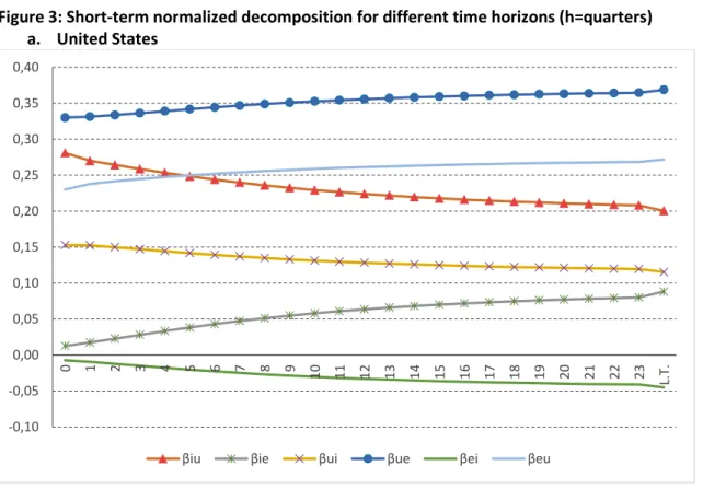
For the United States, Figure 3a shows that the outflow from unemployment into employment
(ue) starts off as the most relevant component, increases its importance monotonically along
the path to the steady-state, and it is not outweighed by the contribution of any other transition.
This result indicates that this transition rate is the most important transition for the dynamics of
unemployment in the United States, even without imposing the assumption that the current
unemployment rate is closely approximated by its steady-state value.
Changes in the contributions were also heterogeneous across the transitions rates. There is a
reversal of the rankings between the flows from employment into unemployment (eu) and from
inactivity into unemployment (iu). Although the transition from a job into unemployment
accounts for a (slightly) smaller contribution in the short-run (ℎ = 0), it surpasses the
contribution of transitioning from inactivity into unemployment from the seventh quarter (ℎ =
6) onwards. It is also noticeable that there are quite distinct trajectories of the contributions of the flow from inactivity into employment (ie) and of its reverse flow (ei): they start off displaying
negligible contributions; and while the contribution of moving into employment directly from
inactivity grows almost linearly, the contribution of the reverse flow displays a downward
trajectory and becomes increasingly negative towards the steady state.
Figure 3: Short-term normalized decomposition for different time horizons (h=quarters) a. United States
-0,10 -0,05 0,00 0,05 0,10 0,15 0,20 0,25 0,30 0,35 0,40
0 1 2 3 4 5 6 7 8 9
10 11 12 13 14 15 16 17 18 19 20 21 22 23 L.T.
b. Brazil
The contributions of the transition rates also display a rich pattern for the case of Brazil, as
shown in Figure 3b. There is a sharp rise in the importance of the flow from employment into
unemployment (eu) and a rise followed by a decline in the contribution of the flow from
inactivity into unemployment (iu). Similar to that in the United States, the relative importance
of these two flows also changes along the path to the steady state. In the Brazilian case, the
inflow from employment into unemployment displays a much smaller contribution in the short
run (ℎ = 0). It outweighs the contribution of the inflow from inactivity into unemployment in
the fifteenth quarter (ℎ = 14) and ends up accounting for the largest share of all components
of the decomposition. There is also a notable change in the relative importance of the transition
from employment into inactivity (ei). It initially ranks as one of the least important components
but surpasses the contributions of other transitions between the fifth and the eight quarters to
eventually become the third most important contributor to the dynamics of unemployment.
5. Conclusion
We devise a decomposition method for the cyclical fluctuations in the level of the
unemployment rate that is not based on the assumption typically made in the literature that the
current rate of unemployment is closely approximated by its steady-state value. Our method
explicitly decomposes the cyclicality in the unemployment rate into a part that is due to the
influence of lagged unemployment rate and into the contributions of the contemporaneous
transitions rates across the different states of the labor market. The method is flexible in that it
0,0 0,1 0,1 0,2 0,2 0,3 0,3 0,4 0,4 0,5
0 1 2 3 4 5 6 7 8 9
10 11 12 13 14 15 16 17 18 19 20 21 22 23 L.T.
allows one to gauge the contributions of these components over different time horizons. Under
regular conditions on the transition matrix, the influence of the lagged unemployment converge
to zero and the contributions of the current transition rates converge to their long-term
analogues in the conventional steady-state decomposition. In that sense, the conventional
steady-state decomposition can be regarded as a special case of our decomposition method.
Using data for the United States and for Brazil, our decomposition results reveal a rich pattern
for the contributions of the initial conditions and the transition rates along the path to the steady
state. These differences in the trajectories of the contributions are sufficiently strong to change
the ranking of some transitions rates in both countries. These qualitative changes are more
significant for Brazil than for the United States. Our results also evince that the steady state
approximation of the unemployment rate performs relatively worse in the former country. We
take these findings as supporting evidence for considering the use of projected unemployment
rate over shorter time horizons as an alternative to the steady state approximation. Our
decomposition results also reveal that, though lagged unemployment account for a large share
in the short run, they quickly lose importance over time to explain the movements in the
unemployment rate in both countries. We believe that by unveiling the importance of the
driving forces of unemployment variability without relying on the steady-state assumption, our
decomposition method provides a useful tool for the analysis of unemployment dynamics in all
countries, regardless of the degree of flexibility in their labor markets.
References
Attuy, G.M. (2012): Ensaios sobre Macroeconomia e Mercado de Trabalho, PhD Thesis,
Departamento de Economia, Universidade de São Paulo.
Blanchard, O. and Diamond, P. (1990) The Cyclical Behavior of the Gross Flows of US Workers,
Brookings Paper on Economic Activity, v.2, pp. 85-143.
Darby, M., Haltiwanger, J., and Plant, M. (1986) The Ins and Outs of Unemployment: The Ins
Win, NBER Working Paper 1997.
Elsby, M.; Michaels, R.; e Solon, G. (2009) The Ins and Outs of Cyclical Unemployment, American
Economic Journal: Macroeconomics, v.1, pp. 84-110
Elsby, M. Hobijn, B. e Sahin, A. (2013) Unemployment Dynamics in the OECD, The Review of
Economics and Statistics, v.95, pp. 530-548
Fujita, S. e Ramey, G. (2009) The Cyclicality of Separation and Job Finding Rate, International
Gomes, P. (2015) The Importance of Frequency in Estimating Labor Market Transition Rates, IZA
Journal of Labor Economics, DOI 10.1186/s40172-015-0021-9.
Hall, R. (2005) Job Loss, Job Finding, and Unemployment in the U.S. Economy over the Past Fifty
Years, in M. Gertler and K. Rogoff (eds), NBER Macroeconomics Annual, 101-137, MIT Press,
Cambridge.
Petrolongo, B. e Pissarides, C. (2008): The Ins and Outs of European Unemployment, American
Economic Review, 98: 256-262.
Shimer, R. (2007) Reassessing the Ins and Outs of Unemployment, NBER Working Paper 13421.
Shimer, R. (2012) Reassessing the Ins and Outs of Unemployment, Review of Economic
Dynamics, 15: 127-148.
Yashiv, E. (2007) U.S. Labor Market Dynamics Revisited, Scandinavian Journal of Economics, 109:
779-806.
Zylberstajn, E. and Portela, A. S. (2016) The Ins and Outs of Unemployment in a Dual Labor
Appendix:Deriving the convergence to the steady state
For each period 𝑡, let 𝜋𝑡 be the transition matrix, 𝑝𝑡 the state probability vector, and 𝑝𝑡∗ its
correspondent steady-state vector.
Let the canonical decomposition of the transition matrix be expressed by 𝜋𝑡 = 𝛾𝑡Λ𝑡γ𝑡−1, where
𝛾𝑡 represents the eigenvectors and Λ𝑡 the diagonal matrix of eigenvalues. As the sum of the
columns of 𝜋𝑡 is equal to 1, it has incomplete rank. In the case of a model with 3 states, 𝜋𝑡 has
rank equal to 2 and therefore Λ𝑡 has two eigenvalues whose values are less than 1 and one
eigenvalue equal to 1, where the corresponding eigenvector has all components with equal
values. This has been confirmed in our empirical analysis for both the United States and Brazil.
Let Λ𝑡 = 𝜒 +𝑡, where 𝜒 = 𝑑𝑖𝑎𝑔(0,0,1) and 𝑡 = 𝑑𝑖𝑎𝑔(𝜆1𝑡, 𝜆2𝑡, 0), with 𝜆1𝑡 < 1 and 𝜆𝑡2< 1. Denoting the state probability vector for the current period by 𝑝𝑡, the projection of 𝑝 for ℎ
periods ahead is given by the following:
𝑝𝑡+ℎ = 𝜋𝑡ℎ𝑝𝑡= 𝛾𝑡Λℎ𝑡𝛾𝑡−1𝑝𝑡 = 𝛾𝑡( 𝜒ℎ+𝑡ℎ)𝛾𝑡−1𝑝𝑡 = (𝐴𝑡+ 𝐴𝑡+ℎ)𝑝𝑡,
where
𝐴𝑡 = 𝛾𝑡𝜒ℎ𝛾
𝑡−1= (𝑎𝑡 𝑎𝑡 𝑎𝑡), and, 𝐴𝑡𝑝𝑡 = (𝑎𝑡 𝑎𝑡 𝑎𝑡)𝑝𝑡 = 𝑎𝑡
for any initial state 𝑝𝑡 since the sum of the components of 𝑝𝑡 is 1, and
𝐴𝑡+ℎ= (𝛾𝑡𝑡ℎ𝛾
𝑡−1) is a matrix that converges to the zero matrix as ℎ grows to infinity. Thus 𝑝𝑡+ℎ = 𝑎𝑡+ 𝐴𝑡+ℎ𝑝𝑡 and 𝑙𝑖𝑚ℎ→∞𝑝𝑡+ℎ= 𝑎𝑡, where 𝑎𝑡 represents the steady-state vector of
the state-probability, i.e., 𝑎𝑡 = 𝑝𝑡∗.
Now, if 𝑝𝑡+ℎ converges to 𝑝𝑡∗, then any well-behaved function of 𝑝𝑡+ℎ, say 𝑔(𝑝𝑡+ℎ), should
converge to 𝑔(𝑝𝑡∗). In particular, the unemployment rate function 𝑢(𝑝𝑡+ℎ) = 𝑢(𝜋𝑡ℎ𝑝𝑡) should
converge to 𝑢(𝑝𝑡∗) = 𝑢(𝐹(𝜋𝑡)).
Following Shimer (2012), the steady-state unemployment rate 𝑢(𝐹(𝜋𝑡)) can be decomposed
into a sum of terms, one of which can be represented by 𝑢(𝐹(𝜓(𝜋𝑡(𝑖, 𝑗); 𝜋̅)) − 𝑢(𝐹(𝜋̅)), where
(𝑖, 𝑗) corresponds to a transition between the state 𝑖 to a state 𝑗 ≠ 𝑖 and the matrix
𝜓(𝜋𝑡(𝑖, 𝑗); 𝜋̅) was defined in equation (18) in the text. The contribution of the transition (𝑖, 𝑗) to
steady-state unemployment is given by
𝛽𝑖𝑗∗ =𝑐𝑜𝑣〈𝑢(𝐹(𝜓(𝜋𝑣𝑎𝑟(𝑢(𝐹(𝜋𝑡(𝑖,𝑗);𝜋̅)),𝑢(𝐹(𝜋𝑡)) 𝑡))〉. (A1)
The prediction of the unemployment rate for ℎ periods ahead can be written as equation (20)
𝑢𝑡+ℎ ≅ 𝜅ℎ+ [𝑢(𝜋̅ℎ+1𝑝𝑡−1) − 𝜅ℎ] + ∑ {𝑢𝑖≠𝑗 (𝜓ℎ+1(𝜋𝑡(𝑖, 𝑗); 𝜋̅)𝑝̅) − 𝜅ℎ} = 𝜅ℎ+ 𝑢0𝑡+ℎ+ ∑ 𝑢𝑖≠𝑗 𝑖𝑗𝑡ℎ , ∀ℎ = 0,1,2, ….
We have contributions from the following terms to the projected unemployment rate:
transition (𝑖, 𝑗): 𝛽𝑖𝑗ℎ=𝑐𝑜𝑣〈𝑢[𝜓𝑡ℎ+1(𝜋𝑡(𝑖,𝑗);𝜋̅)𝑝̅],𝑢𝑡+ℎ〉
𝑣𝑎𝑟(𝑢𝑡+ℎ) ; (A2)
initial state of the labor market: 𝛽0ℎ=𝑐𝑜𝑣〈𝑢(𝜋̅ℎ+1𝑝𝑡−1),𝑢𝑡+ℎ〉
𝑣𝑎𝑟(𝑢𝑡+ℎ) . (A3)
As 𝜓(𝜋𝑡(𝑖, 𝑗); 𝜋̅) is a transition matrix, the previous convergence results also apply here, and
thus 𝑢(𝜓ℎ+1(𝜋𝑡(𝑖, 𝑗); 𝜋̅)𝑝̅) converges to 𝑢(𝐹(𝜓(𝜋𝑡(𝑖, 𝑗); 𝜋̅)). Hence, all the elements in (A2)
converge to their counterparts in (A1) (i.e., 𝛽𝑖𝑗ℎ converges to 𝛽𝑖𝑗∗, ∀𝑖 ≠ 𝑗) when ℎ grows to infinity.
As for 𝛽0ℎ, note that 𝜋̅ℎ+1𝑝𝑡−1= (𝑎 + 𝐴ℎ)𝑝𝑡−1= 𝑎 + 𝐴ℎ𝑝𝑡−1. As 𝐴ℎ𝑝𝑡−1 converges to zero
with ℎ, 𝛽0ℎ=𝑐𝑜𝑣〈𝑢(𝑎+𝐴ℎ𝑝𝑡−1),𝑢𝑡+ℎ〉