Coloring and Independent-Set Optimization Transitions
Valmir C. Barbosa*
Programa de Engenharia de Sistemas e Computac¸a˜o, Instituto Alberto Luiz Coimbra de Po´s-Graduac¸a˜o e Pesquisa de Engenharia (COPPE), Universidade Federal do Rio de Janeiro, Rio de Janeiro, Brazil
Abstract
Background:Given an undirected graph, we consider the two problems of combinatorial optimization, which ask that its chromatic and independence numbers be found. Although both problems are NP-hard, when either one is solved on the incrementally denser graphs of a random sequence, at certain critical values of the number of edges, it happens that the transition to the next value causes optimal solutions to be obtainable substantially more easily than right before it.
Methodology/Principal Findings:We introduce the notion of a network’s conduciveness, a probabilistically interpretable measure of how the network’s structure allows it to be conducive to roaming agents, in certain conditions, from one portion of the network to another. We demonstrate that the performance jumps of graph coloring and independent sets at the critical-value transitions in the number of edges can be understood by resorting to the network that represents the solution space of the problems for each graph and examining its conduciveness between the non-optimal solutions and the optimal ones. Right past each transition, this network becomes strikingly more conducive in the direction of the optimal solutions than it was just before it, while at the same time becoming less conducive in the opposite direction.
Conclusions/Significance:Network conduciveness provides a useful conceptual framework for explaining the performance jumps associated with graph coloring and independent sets. We believe it may also become instrumental in helping clarify further issues related to NP-hardness that remain poorly understood. Additionally, it may become useful also in other areas in which network theory has a role to play.
Citation:Barbosa VC (2010) Network Conduciveness with Application to the Graph-Coloring and Independent-Set Optimization Transitions. PLoS ONE 5(7): e11232. doi:10.1371/journal.pone.0011232
Editor:Enrico Scalas, University of East Piedmont, Italy
ReceivedMarch 17, 2010;AcceptedMay 28, 2010;PublishedJuly 8, 2010
Copyright:ß2010 Valmir C. Barbosa. This is an open-access article distributed under the terms of the Creative Commons Attribution License, which permits unrestricted use, distribution, and reproduction in any medium, provided the original author and source are credited.
Funding:This work was partially supported by Conselho Nacional de Desenvolvimento Cientı´fico e Tecnolo´gico (CNPq), Coordenac¸a˜o de Aperfeic¸oamento de Pessoal de Nı´vel Superior (CAPES), and a Cientista do Nosso Estado grant from Fundac¸a˜o Carlos Chagas Filho de Amparo a` Pesquisa do Estado do Rio de Janeiro (FAPERJ). The funders had no role in study design, data collection and analysis, decision to publish, or preparation of the manuscript.
Competing Interests:The author has declared that no competing interests exist.
* E-mail: [email protected]
Introduction
The past decade has seen an impressive growth in the science of complex networks, understood as the branch of scientific inquiry which, by merging well established notions and techniques from the theory of graphs and from statistical physics, addresses the interplay of structure and function in the large, essentially unstructured networks that occur in a wide variety of domains. The latter have encompassed several instances in many biological, social, and technological fields, and have yielded an equally variegated array of results that the reader can now refer to in books and paper collections such as [1–3].
One common methodological thread in all these studies has been the definition of a graph to represent the interactions among certain entities in the domain of interest, followed by the analysis of mathematical descriptors of some of the graph’s properties as averages over a number of graphs generated according to some random-graph model thought to represent the phenomenon under consideration. Thus have emerged important finds regarding the characterization of some networks as small-world structures, or as scale-free structures, as well as powerful structural indicators of a graph’s nature, such as its clustering coefficient and various centrality-related quantities.
Here we introduce another indicator of a graph’s properties, called its conduciveness. Given a directed graphDof node setN, the conduciveness ofD is defined with respect to two subsets A
andBofN. Letdidenote the out-degree of nodeiinD(the node’s number of outgoing edges) and define i’s B-bound out-degree, denoted by dB
i, to be its number of outgoing edges whose
heads are members of B (i.e., edges that lead from i to some member ofB). The conduciveness ofDfromAtoBis denoted by CondA,B(D)and given by
CondA,B(D)~
P
i[Ad B i
P
i[Adi
: ð1Þ
Clearly,0ƒCondA,B(D)ƒ1.
This definition of a directed graph’s conduciveness can be easily interpreted in the context of hypothetical agents inhabiting the graph at its nodes but free to roam to other nodes by taking steps that follow edges along their directions. Specifically,CondA,B(D)
this probability is higher than for another is regarded as more conducive to setBfrom setAthan that other graph.
Our initial motivation for the introduction of this definition has been its potential application to explain some phenomena related to the complexity of solving certain problems of combinatorial optimization. Normally such a problem is defined on the setVof the feasible solutions to the problem, using a real function f
defined overVaccording to which an optimal member ofVis to be found (one for whichf is minimum or maximum over all ofV, depending on the problem). Many such problems are NP-hard, meaning that finding optimal solutions to them is at least as hard as solving any of the decision problems that constitute the class NP (those whose solutions, should they somehow be provided at no cost and turn out to be affirmative, could be checked to be correct in polynomial time [4]). That no polynomial-time deterministic algorithm has ever been found to solve an NP-hard problem is normally taken as a sign of computational intractability as problem instances grow large.
This, however, is to be taken with caution. The class NP can be viewed as a complex hierarchy of subclasses [5], which may ultimately help account for what is observed in practice: some NP-hard problems are solvable much more efficiently than others; more strikingly, two similarly sized instances of the same NP-hard problem may require considerably different amounts of computational effort to be solved. A way to illustrate this that is useful in the context of this paper is based on the following. Let there be n nodes and, for
M~n(n{1)=2, consider a sequence C~SG1,G2,. . .,GMT of
undirected graphs on these nodes. Form~1, Gm has one single edge joining two randomly chosen nodes andn{2isolated nodes. For1vmƒM,Gmis obtained fromGm{1by placing a further edge
between two randomly chosen nodes that are not already joined by an edge; soGm hasmedges and, for relatively smallm, may also have isolated nodes.
The crucial observation is that, as first documented in [6,7] in the wake of what was done earlier for some NP-hard decision problems [8–12], there exist NP-hard optimization problems for which practically every attempted algorithm, deterministic or otherwise, undergoes sharp performance variations when applied to the graphs inCfor increasing values ofm. These variations refer to jumps in how long it takes the algorithm to reach an optimal solution and happen at well-defined critical values ofmgivenC. The same initial reporters of these phenomena also offered tentative explanations related to the nature and structure of the corresponding Vsets (one for each of the M graphs in C), but those have lacked full consistency owing to normalization difficulties as the sizes of those sets grow along withm[7]. It has also been a difficulty that the values ofmat which the jumps occur tend to be different ifCis changed, so the aforementioned analyses have only addressed single graph sequences and therefore lack statistical significance as well.
We have found that the notion of a directed graph’s conduciveness, as introduced above, has an important role to play in elucidating the nature of these performance jumps. The fundamental idea is, for each m, first to identify an appropriate descriptor of the feasible solutions to the problem that is being posed onGm. This will give us theVset for that particular m, henceforth denoted by Vm. Then we identify some primitive
operation on the members ofVmthat may be used to transform
one of them into another. Every two members ofVmthat are thus
related constitute an ordered pair; collectively, all such pairs constitute the set that we denote byEm. The directed graph whose conduciveness we study, denoted by Dm, has node set Vm and
edge set Em. This graph embodies all primitive steps that an optimum-seeking algorithm may take to solve the problem onGm.
Form~1,2,. . .,M, we study the conduciveness ofDm from the nodes inVmthat do not represent optimal solutions to those that
do.
By its very nature as a probability, this conduciveness ofDmhas none of the normalization problems alluded to above. As we will see, it also allows for some multiplicity of events to be investigated for statistical significance, though only to a limited extent. This is because in general the edges ofDmcan only be found through the explicit enumeration and testing of several pairs of members of Vm, which in most cases is a very large set even for very small
values ofn. We then see that there exist severe time constraints on the generation of the Dm graphs for multiple instances of the sequenceC, and consequently constraints on the largest value ofn
that can realistically be used. We note, moreover, that seldom can
Dm be fully stored, which limits the properties that can be analyzed.
We target the same two optimization problems as [7], namely the problem of coloring the nodes of an undirected graph optimally and that of finding one of its maximum independent sets. Aside from the fact that they are both paradigmatic NP-hard optimization problems, our choice of them has also been influenced by the remarkable fact that, for each value ofm, it is possible to define a singleVmset for both problems, thus allowing
the study of their performance jumps to be conducted in a peculiarly interrelated fashion.
Methods
The chromatic number of an undirected graphGonnnodes, denoted byx(G), is an integer between 1 and n indicating the smallest number of distinct colors (labels) that can be used to tag the nodes ofGin such a way that every node gets exactly one color and no two nodes connected by an edge get the same color. The independence (or stability) number of G, denoted by a(G), is likewise an integer between1and n and indicates the size of a largest independent subset ofG’s node set, that is, a largest subset of nodes containing no two nodes connected by an edge [13]. Finding either number is an NP-hard problem [4].
The two problems can be reformulated in such a way that their setsVof feasible solutions are in fact the same set. To see this, first let an orientation ofGbe an assignment of directions toG’s edges, that is, one of the ways in whichGcan be turned into a directed graph. An orientation is acyclic if it contains no directed cycles (i.e., it is never possible to return to a node after moving away from it along the directions of the edges). Every acyclic orientation ofG
yields a number of colors to tag the nodes ofGlegitimately, and likewise an independent set of G. Conversely, every legitimate assignment of colors to the nodes ofGyields an acyclic orientation ofG, and so does every independent set ofG. The proofs that back up these statements are not simple [14], but accepting them clearly implies that both findingx(G)and findinga(G)can be formulated based on sharing the Vset defined as the set of all the acyclic orientations ofG.
The precise relationships implied by the proofs in [14] are the following. Letv be an acyclic orientation of G. Let Depth(v) denote the number of nodes on a longest directed path in G
according tov, henceforth referred to simply as the depth ofv. Then
x(G)~min
v[V
Depth(v), ð2Þ
simply as the width ofv. Then
a(G)~max
v[V
Width(v), ð3Þ
meaning thata(G)is the width of the widest member ofV. It also emerges from those same proofs (but see [15,16] for explicit accounts of the corresponding algorithms) that, given v, both Depth(v) and Width(v) can be computed in polynomial time. So, by Equations (2) and (3), the NP-hardness of the two problems in question is to be attributed to the inherent difficulty of searching insideVfor an optimalvin each case. Following the general outline provided in the previous section, we continue by defining the directed graphDof node setVwhose edge set,E, is to be set up to reflect some primitive relationship among the members ofVthat can be used to transform each one into some other.
There are certainly several ways in which an acyclic orientation,
sayv, can be turned into another, sayv’. One possibility that has
become popular in several task scheduling applications is to turn one or more of the sinks ofv(nodes with no outgoing edges) into sources (nodes with no incoming edges) and then let the resulting orientation bev’(clearly acyclic, given the acyclicity ofv). We eschew this choice for two reasons. The first one is that it entails several direction reversals for one single transformation, which then seems hard to qualify as primitive. The second reason is that, under such sink-to-source transformations, the resulting D is almost always a fragmented graph (i.e., there exist pairs of nodes that are unreachable from each other even if edge directions are ignored) [17]. Since our interest is in the conduciveness ofDwith respect to certain subsets ofV, it seems that starting out with a fragmented D is bound to produce results somewhat devoid of meaning.
Our definition of the edge set E of D is then the following. Givenv[V, an edge exists directed fromvto somev’[Vif and only ifv’results from reversing the direction of exactly one of the edges ofGas oriented byv. Of course, if(v,v’)[Eholds, then so does (v’,v)[E. Moreover, it now holds that D is strongly connected, that is, a directed path exists from any node to any other. (To see that the latter holds, consider that, if it does not, then there have to existv,v’[Vwith the following property. IfS is the set of edges inGon whose directionsvandv’disagree, then the individual direction reversal of any edgee[Screates a directed cycleCin the resulting orientation. But sincev’is acyclic,Cmust also contain another of the edges of S, say e’, and this edge’s direction must oppose that of eon C. Notice, however, thatC
comprises at least three edges, so reversing the direction ofe’alone would create no directed cycle. This contradicts the existence of thev,v’pair with the assumed property.)
HandlingDcomputationally, though, is a difficult matter owing to both its number of nodes and the explicit way in which its edges must be enumerated. The number of nodes, which is the number of distinct acyclic orientations of G, is given by a surprising application of the so-called chromatic polynomial ofG[18] and, fornfixed, grows rapidly from the two orientations allowed by the case of one single edge to then!orientations that a graph with all possibleM edges onnnodes admits. As for discovering the edges ofDthat outgo from a particular orientationv, there is in general no alternative but to try and reverse the directions of all edges of
G, one by one with respect to whatvstipulates, checking for each one whether the resulting orientation is itself a member ofV.
GivenG, we enumerate the members of V by the algorithm given in [19] but store each one only while recording some of its properties for later use. For eachvthat is output by the algorithm,
we calculateDepth(v),Width(v), its out-degreedvinD, and its
B-bound out-degree dB
v. Here B depends on which problem is being addressed. If it is the coloring problem, thenBis the subset ofVcomprising orientations whose depths are all equal tox(G). If it is the independent-set problem, thenBis the subset ofVwhose orientations all have width a(G). For simplicity, whenever the context allows we refer todv as a full degree and to dvB as an optimum-bound degree. Note that each full degree is an integer between1 and the number of edges ofG. An optimum-bound degree, in turn, is an integer between0and again the number of edges ofG.
Scarce though they may be, these recorded properties of D
allow for some useful statistics to be computed, in addition to allowing for the direct calculation of some useful conduciveness figures forDas per Equation (1). Usingdx,yto denote Kronecker’s
delta function of the integers x and y, and DXD to denote the cardinality of setX, these statistics are:
N
The distribution of full degrees inD, given byP(k)~ P
v[Vddv,k
DVD ð4Þ
for every possible full degreek.
N
The distribution of depths inD, given byQ(u)~ P
v[VdDepth(v),u
DVD ð5Þ
for every possible depthu.
N
The distribution of widths inD, given byR(v)~ P
v[VdWidth(v),v
DVD ð6Þ
for every possible widthv.
N
The joint distribution of full degrees and depths inD, given byS(k,u)~ P
v[Vddv,kdDepth(v),u
DVD ð7Þ
for every possible full degreekand depthu.
N
The joint distribution of full degrees and widths inD, given byT(k,v)~ P
v[Vddv,kdWidth(v),v
DVD ð8Þ
for every possible full degreekand widthv.
Additional statistics are PB(k), SB(k,u), and TB(k,v), defined
analogously to the above but for optimum-bound degrees (that is, substitutingdB
vfordvin the corresponding definitions). Note also that, whenever theGin question is one of theGm graphs of the sequenceCintroduced previously, we alter the notation of these statistics by adopting the subscriptmfor them as well (consistently with the graphDmof node setVmand edge setEm, all introduced
earlier but now with the specific meanings given in this section for
D,V, andE, respectively).
Results
Let us then look at one single sequence C~SG1,G2,. . .,GMT
to find x(G1),x(G2),. . .,x(GM) and a(G1),a(G2),. . .,a(GM)
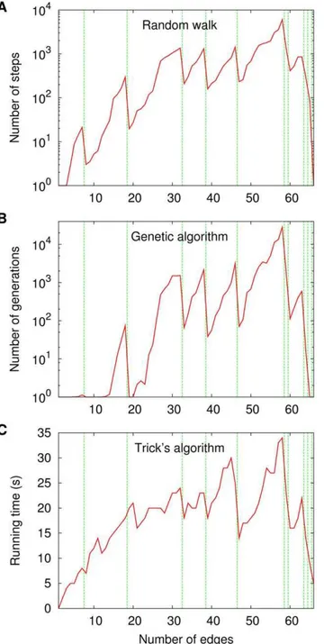
per-form. Results on finding the chromatic numbers are given in Figure 1; those on finding the independence numbers are in Figure 2.
Figure 1 contains performance data on three algorithms. First is a simple random walker, which for eachmstarts at a randomly chosen acyclic orientation inVm and then at each step traverses
one of the edges that outgo from its current acyclic orientation in
Figure 1. Performance of three algorithms to find the
chromatic numbers of the graphs in C. Data are given for a
random walker (A), a genetic algorithm (B), and Trick’s implementation [21] of the algorithm in [22] (C). The data shown for part A are averages over 10 000 independent runs. The genetic algorithm is the one described in the caption to Figure 15 in [7], parameter values included. It is based on viewing each acyclic orientation as an individual in a population and on letting selection favor those individuals that come closer to having optimal depth. It also relies on effecting acyclicity-preserving crossover and mutation operations. The data shown for part B are averages over 100 independent runs. Trick’s algorithm assigns colors to nodes as a function of the colors their neighbors already have. doi:10.1371/journal.pone.0011232.g001
Figure 2. Performance of three algorithms to find the
independence numbers of the graphs inC.Data are given for a
random walker (A), a genetic algorithm (B), and Johnson’s implemen-tation [23] of the algorithm in [24] (C). The data shown for part A are averages over 10 000 independent runs. The genetic algorithm is the one described in the caption to Figure 15 in [7], parameter values included. It is based on viewing each acyclic orientation as an individual in a population and on letting selection favor those individuals that come closer to having optimal width. It also relies on effecting acyclicity-preserving crossover and mutation operations. The data shown for part B are averages over 100 independent runs. Johnson’s algorithm follows a simple branch-and-bound strategy.
the setEm, thus reaching another acyclic orientation. Performance data are then given for a genetic algorithm operating onVm, and
then for a deterministic algorithm whose operation is not based on
Dmat all. The random walker and the genetic algorithm stop upon hitting the first acyclic orientationvfor whichDepth(v)~x(Gm), with the provision thatx(Gm)is known beforehand from running the third algorithm first. The data on all three algorithms are shown in the three parts of Figure 1 against a backdrop of vertical lines, each marking the critical number of edges right past which an increase in the chromatic number occurs: for 1ƒmvM, if x(Gmz1)~x(Gm)z1, then a vertical line is drawn at the abscissa
mz0:5. The chromatic numbers of the graphs in Cnecessarily increase by 1 past each critical value, from x(G1)~2 through
x(GM)~n, therefore there aren{2vertical lines all told. A similar arrangement holds for Figure 2, whose setting differs from that of the previous one in that now both the random walker and the genetic algorithm stop upon finding v[Vm such that Width(v)~a(Gm), once again given thata(Gm)is known a priori from running the deterministic algorithm first. There is also an important difference regarding the changes in the graphs’ independence numbers, which now necessarily decrease by1past each critical number of edges, from a(G1)~n{1 through
a(GM)~1, thus totalingn{2decreases as well. So, in Figure 2, the vertical lines marking the decreases are drawn at the abscissae
mz0:5such thata(Gmz1)~a(Gm){1.
Given these critical numbers of edges, which depend on whether the graph-coloring or the independent-set problem is being addressed, we henceforth refer simply as a transition to the addition of one edge to the graph beyond some critical number. An explicit distinction between the two problems is made whenever needed for clarity. For the graph sequenceC, Figure 3 summarizes the stepwise growth of the chromatic number at the corresponding transitions, and similarly the diminution of the independence number. The figure also highlights the progress of the number of acyclic orientations as the number of edges increases. Clearly, the number of acyclic orientations grows rather rapidly and achieves the order of102as early as the first transition
related to the chromatic number.
Parts A and B of both Figures 1 and 2 refer to methods which work on the setsVmof acyclic orientations of the graphsGm, either
making explicit use of the structure of eachDm(which the random walker does) or allowing for longer jumps as the orientations undergo the crossover and mutation operations prescribed by the genetic algorithm. The data displayed in the corresponding four panels often have in common the property that the occurrence of a transition, say fromm’to m’z1 edges, causes the algorithm in question to perform significantly better onGm’z1than onGm’, and then increasingly poorly through the following values ofm until the next transition, if any, is reached. This difference in performance is sometimes quite marked, involving improvements by at least one order of magnitude.
What is perhaps more curious is that the same behavior is also present in Figure 1C, which refers to a deterministic algorithm to find chromatic numbers that does not rely on theDmgraphs (in fact, this algorithm’s underlying strategy makes no reference at all to the acyclic orientations of the graph whose chromatic number it is seeking). Informally, then, this seems to indicate that the characteristic performance jumps at the transitions are inherent to the optimization problem itself (and only marginally, if at all, dependent upon how its feasible solutions are represented). It also seems to confer to the Dm graphs some of the primitive representational character we sought in the beginning. However, Figure 2C, which also refers to a deterministic algorithm that does not operate on acyclic orientations, only now to find the graph’s independence number, shows none of the effects on performance at the transitions that the random-walk and genetic-algorithm approaches exhibit. The reason for this is that, despite being just as nominally NP-hard as the problem of finding chromatic numbers, finding independence numbers is easier in practice than that other problem. What this means is that, in order for the transitions’ effects on performance to show, substantially higher values ofnare needed (cf. Figure 9 in [7]).
We then proceed on the premise that the sequence of Dm
graphs form~1,2,. . .,Mcontains information enough to explain the performance jumps at the transitions, even though quantita-tively we can only resort to what can be derived from each graph’s nodes’ depths, widths, and out-degrees. One initial indication that this makes sense comes from investigating the mutual information of pairs of random variables associated with eachDm. Given two discrete random variables and the joint distribution of their values, their mutual information is a measure of how much fixing the value of one of them reduces the uncertainty on the value of the other [20]. Just like Shannon’s entropy, mutual information is expressed in (information-theoretic) bits.
In the context of findingx(Gm), two discrete random variables of interest are those that give the out-degree and the depth of a randomly chosen node ofDm. Their joint distribution isSm(k,u)in the case of full degrees,SB
m(k,u) in the case of optimum-bound
degrees, both introduced earlier. Their mutual information is, respectively for each case, given by
Im~X
m
k~1
Xn
u~2
Sm(k,u)log2
Sm(k,u)
Pm(k)Qm(u) ð9Þ
and
ImB~
Xm
k~0
Xn
u~2
SmB(k,u)log2
SB m(k,u) PB
m(k)Qm(u)
: ð10Þ
If the problem is to finda(Gm), then the two random variables give the node’s out-degree and its width. Their joint distributions are
Tm(k,v) and TB
m(k,v), once again depending on whether full or Figure 3. Chromatic- and independence-number variations at
the transitions alongC.Chromatic-number increases and
indepen-dence-number decreases occur by single units at the corresponding transitions, while the number of acyclic orientations grows steadily with the number of edges.
optimum-bound degrees are referred to. The respective measures of mutual information are
Jm~X
m
k~1
Xn{1
v~1
Tm(k,v)log2
Tm(k,v)
Pm(k)Rm(v) ð11Þ
and
JmB~X
m
k~0
Xn{1
v~1
TmB(k,v)log2
TB m(k,v) PB
m(k)Rm(v)
: ð12Þ
For the same sequence C we have considered so far in this section, and following the same conventions as Figures 1 and 2 with regard to marking with vertical lines the values ofmat which x(Gm)ora(Gm)changes along the sequence, we show in Figure 4 the progress of these four mutual information functions, in part A for graph coloring, in part B for independent sets. Note, in all cases, that although consistently less than one bit, all four functions are nearly always positive, thus providing evidence that, in most
Dm instances, out-degrees of either kind are independent from neither depths nor widths. However, the functions do not seem to behave consistently at the transitions and for this reason offer no direct explanation of what happens there.
It is important to recall that all of Figures 1, 2, 3, 4 refer to the one single sequenceC. They have been offered as illustrations of what is typical, and averaging over multiple graph sequences, which requires that we address the fact that transitions may occur at differentmvalues in different sequences, might blur the reader’s understanding of what the phenomenon is and how mutual information suggests that it has to do with theDmgraphs. We now turn to the role played by graph conduciveness and, after one more single-sequence illustration, do some averaging as properly as possible.
Given a Dm graph, let Vxm denote the subset of Vm whose
members are those of depthx(Gm). Analogously, letVamdenote the
subset ofVmwhose members are those of widtha(Gm). We study
four kinds of conduciveness ofDm, given as follows with reference to Equation (1); we use\to denote set difference.
Cxm, in~CondVm\Vxm,Vxm(Dm); ð13Þ
Cxm, out~CondVx
m,Vm\Vxm(Dm); ð14Þ
Cam, in~CondVm\Vam,Vam(Dm); ð15Þ
Cma, out~CondVam,Vm\Vam(Dm): ð16Þ
Note thatCx, in
m is the conduciveness ofDm from all orientations
that are non-optimal for coloring to those that are optimal,Cx, out
m
the conduciveness in the opposite direction. The situation with
Ca, in
m andCma, outis totally analogous, now regarding optimality for
independent sets. We refer toCx, in
m andCma, inas being inbound, to Cx, out
m andCma, outas being outbound. Note also that, by Equation
(1), and given the antiparallel nature of the edge set ofDm, it holds that
Cx, out
m ~
P
v[Vm\Vxmdv
P v[Vxmdv
Cx, in
m ð17Þ
and
Cma, out~
P
v[Vm\Vamdv
P v[Vamdv
Cma, in: ð18Þ
These, however, imply no obvious relationship between the inbound conduciveness ofDmand its outbound conduciveness for any of the two problems.
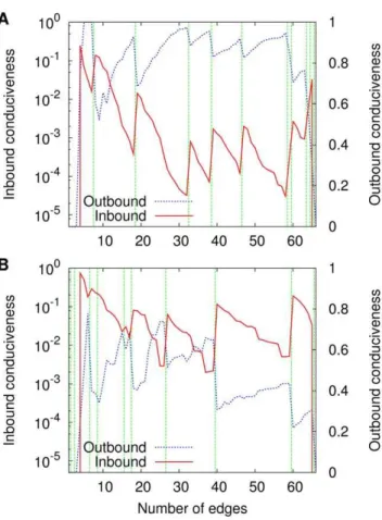
An illustration of the kind of relationship that does hold is given in Figure 5, which results from our last use of the same single sequenceCas heretofore. Strikingly, as the sequence unfolds with increasingm and the changes inx(Gm) (part A of the figure) or a(Gm)(part B of the figure) occur, the inbound conduciveness of
Dm undergoes sudden jumps upwards precisely at the transitions while its outbound conduciveness undergoes downward jumps. The inbound-conduciveness jumps can be seen to encompass at least one order of magnitude in many cases. Between one transition and the next, the inbound conduciveness deteriorates progressively while the outbound conduciveness improves. This is then the key to interpreting the phenomena illustrated in Figures 1 and 2: at the transitions,Dmbecomes markedly more conducive in
Figure 4. Evolution of the mutual information alongC.Data are
given forImandIB
m(A), which refer to coloring, respectively for full and
optimum-bound degrees; and forJmandJBm(B), which likewise refer to
independent sets.
the direction of the optimal orientations and less conducive in the opposite direction; right past a transition through right before the next one happens, Dm tends to become progressively less conducive in the direction of the optima, more conducive in the direction that leads away from them.
Next we study these conduciveness variations as averages over the graph sequences C1,C2,. . .,C15, each comprising graphs on
n~12nodes and generated independently. As noted earlier, even though both the chromatic number and the independence number undergon{2changes each at the transitions in each sequence, the tth transition, for some t[f1,2,. . .,n{2g, may happen at different values ofmfor the different sequences. Some alignment of the transitions is then needed for the averages of interest to be computed; we proceed as follows. If for a given sequence thetth transition related to the chromatic number occurs form~m’, then we calculate the change ratios (Cmx, in’z1{C
x, in
m’ )=C x, in
m’ and
(Cmx, out’z1{C
x, out
m’ )=C x, out
m’ . We do likewise for each transition related to the independence number. If two subsequent transitions related to the chromatic number occur atm~m’andm~m’’wm’, then we also calculate the change ratios (Cmx, in’’ {Cmx, in’z1)=C
x, in
m’z1
and (Cmx, out’’ {Cx, out
m’z1)=C
x, out
m’z1, again proceeding likewise for the
interval between every pair of subsequent transitions related to the independence number. The latter formulae can also be used to calculate change ratios for the interval that precedes the first transition (lettingm’~0andm’’be the value ofmat which the first transition occurs) and the interval that succeeds the last transition (lettingm’be value ofm at which the last transition occurs and
m’’~M). Once all change ratios have been calculated, they can be averaged over the15sequences for each transition (whichever the value ofmis at which it happens to occur in each sequence) and each interval.
These average change ratios are given in Figures 6 and 7, respectively for graph coloring and independent sets. All data in these two figures are presented, as in most previous cases, against a backdrop of vertical lines. These, however, are now equally spaced and refer to the transition numbers, from 1 through n{2, regardless of themvalues at which the transitions themselves are observed in each particular sequence for each problem. Each panel in each figure contains two plots, one with points whose abscissae coincide with those of the vertical lines (this refers to change ratios at the transitions) and one with points whose abscissae stand either halfway between those of two consecutive vertical lines or to the left (right) of the leftmost (rightmmost) vertical line’s abscissa [this refers to change ratios along the intervals between consecutive transitions or before (after) the first (last) transition].
Figures 6A and 7A, which refer to the progress of the inbound conduciveness as the transitions elapse, reveal that at most transitions the upward jumps represent significant fractions of the pre-transition conduciveness values, which often increase manyfold (by a factor of a few tens). On the other hand, the accumulated deterioration in conduciveness that is observed between transitions and in the outermost intervals is in most cases given by a fraction that varies widely depending on the transition,
Figure 5. Evolution of network conduciveness alongC.Data are
given for Cx, in
m and Cxm, out (A), which refer to coloring, respectively
inbound and outbound; and forCa, in
m andCma, out(B), which likewise refer
to independent sets.
doi:10.1371/journal.pone.0011232.g005
Figure 6. Conduciveness change ratios at the graph-coloring
transitions and related intervals.Data are given as averages over
the set of sequencesfC1,C2,. . .,C15gfor both the inbound
ranging practically from nearly no loss of the initial conduciveness inside the interval to nearly total loss.
Figures 6B and 7B, in turn, refer to how the outbound conduciveness values evolve along with the transitions and show that, right at the transitions, conduciveness is lost with respect to the pre-transition values by fractions that amount to losing from about5–10% of it (depending on the problem) to all of it. As we look at the accumulated improvement in conduciveness between transitions and in the outermost intervals, we see that a wide range of possibilities is again present, allowing at one extreme for
practically no improvement and, at the other extreme, for an improvement by about70–90% of the initial conduciveness inside the interval (depending on the problem).
Discussion
The notion of network conduciveness we have introduced is a simple degree-based indicator that can be interpreted as a probability with respect to a particular agent-related dynamics. We believe that, either as defined or as some variant thereof, it may find applications in network studies having to do with the dynamics of populations in networks. Our own application in this paper has been to the field of combinatorial optimization, and then the network in question is representative of the feasible solutions to a particular instance of an optimization problem and of how one may move from one solution to another through as simple a local transformation as possible. We tackled the NP-hard problems of finding an undirected graph’s chromatic and independence numbers and demonstrated how network condu-civeness, when applied to problem representations in the domain of the graph’s acyclic orientations, is capable of helping explain the well-known performance jumps that occur along random sequences of graphs for both problems.
As it happens, though, the networks whose conduciveness we have considered grow very rapidly with the graph’s numbers of nodes and edges, and become themselves very nearly intractable already for small instances of the problems we addressed. We were then limited in our computational experiments to using graphs on 12 nodes exclusively and to averaging results on 15 random sequences of graphs. For the sake of the record, with current technology all experiments required nearly two months on twenty processors. So, as much as we think that there is great potential usefulness to the notion of a network’s conduciveness, further progress with the particular application we chose requires considerable further effort so that larger graphs and better statistical significance can be aimed at. On the other hand, we regard the first steps we have taken as very significant: to the best of our knowledge, no other study has addressed the intricacies of NP-hard optimization problems from the perspective of network theory applied to the structure that underlies the problems’ sets of feasible solutions.
Author Contributions
Conceived and designed the experiments: VB. Performed the experiments: VB. Analyzed the data: VB. Contributed reagents/materials/analysis tools: VB. Wrote the paper: VB.
References
1. Bornholdt S, Schuster HG, eds (2003) Handbook of Graphs and Networks. Weinheim, Germany: Wiley-VCH.
2. Newman M, Baraba´si AL, Watts DJ, eds (2006) The Structure and Dynamics of Networks. Princeton, NJ: Princeton University Press.
3. Bolloba´s B, Kozma R, Miklo´s D, eds (2009) Handbook of Large-Scale Random Networks. Berlin, Germany: Springer.
4. Garey MR, Johnson DS (1979) Computers and Intractability: A Guide to the Theory of NP-Completeness. New York, NY: W. H. Freeman.
5. Johnson DS (1990) A catalog of complexity classes. In: van Leeuwen J, ed. Handbook of Theoretical Computer Science. Cambridge, MA: The MIT Press, volume A. pp 67–161.
6. Slaney J, Walsh T (2001) Backbones in optimization and approximation. In: Proceedings of the Seventeenth International Joint Conference on Artificial Intelligence. San Francisco, CA: Morgan Kaufmann Publishers. pp 254–259. 7. Barbosa VC, Ferreira RG (2004) On the phase transitions of graph coloring and
independent sets. Physica A 343: 401–423.
8. Cheeseman P, Kanefsky B, Taylor WM (1991) Where the really hard problems are. In: Proceedings of the Twelfth International Joint Conference on Artificial Intelligence. San Mateo, CA: Morgan Kaufmann Publishers. pp 331–337.
9. Mitchell D, Selman B, Levesque H (1992) Hard and easy distributions of SAT problems. In: Proceedings of the Tenth National Conference on Artificial Intelligence. Menlo Park, CA: AAAI Press. pp 459–465.
10. Monasson R, Zecchina R, Kirkpatrick S, Selman B, Troyansky L (1999) Determining computational complexity from characteristic ‘phase transitions’. Nature 400: 133–137.
11. Giordana A, Saitta L (2000) Phase transitions in relational learning. Machine Learning 41: 217–251.
12. Culberson J, Gent I (2001) Frozen development in graph coloring. Theoretical Computer Science 265: 227–264.
13. Bondy JA, Murty USR (2008) Graph Theory. New York, NY: Springer. 14. Deming RW (1979) Acyclic orientations of a graph and chromatic
and independence numbers. Journal of Combinatorial Theory B 26: 101–110.
15. Barbosa VC, Assis CAG, do Nascimento JO (2004) Two novel evolutionary formulations of the graph coloring problem. Journal of Combinatorial Optimization 8: 41–63.
16. Barbosa VC, Campos LCD (2004) A novel evolutionary formulation of the maximum independent set problem. Journal of Combinatorial Optimization 8: 419–437.
Figure 7. Conduciveness change ratios at the independent-set
transitions and related intervals.Data are given as averages over
the set of sequencesfC1,C2,. . .,C15g for both the inbound
17. Barbosa VC (2000) An Atlas of Edge-Reversal Dynamics. London, UK: Chapman & Hall/CRC.
18. Stanley RP (1973) Acyclic orientations of graphs. Discrete Mathematics 5: 171–178.
19. Barbosa VC, Szwarcfiter JL (1999) Generating all the acyclic orientations of an undirected graph. Information Processing Letters 72: 71–74.
20. Latham PE, Roudi Y (2009) Mutual information. Scholarpedia 4: 1658.
21. Trick MA (1994) COLOR.C: Easy code for graph coloring. Available http:// mat.gsia.cmu.edu/COLOR/solvers/trick.c.
22. Bre´laz D (1979) New methods to color vertices of a graph. Communications of the ACM 22: 251–256.
23. Johnson DS (1993) dfmax.c: Semi-Exhaustive Greedy Independent Set. Available ftp://dimacs.rutgers.edu/pub/dsj/clique/dfmax.c.