Universidade Nova de Lisboa Faculdade de Ciências e Tecnologia Departamento de Informática
Master Thesis
European Master in Computational Logics
Constraint-based modeling of
Minimum Set Covering: Application to
Species Differentation
David Buezas (32411)
Universidade Nova de Lisboa Faculdade de Ciências e Tecnologia Departamento de Informática
Master Thesis
Constraint-based modeling of
Minimum Set Covering: Application to
Species Differentation
David Buezas (32411)
Superviser: Dr. Pedro Barahona
Work presented in the context of the European Master in Computational Logics, as partial requi-sit for the graduation as Master in Computational Logics.
Acknowledgements
I am very grateful to my supervisor Dr. Pedro Barahona1who, in spite of his tight schedule, found time to guide and help me with his agile mind to overcome the obstacles throughout the whole development of the present dissertation. Also I am in debt with João Almeida2 who first proposed the Species Differentiation Problem and provided clarification about the biological aspects with which this thesis is concerned. My Master studies were supported by the European Master’s Program in Computational Logic (EMCL) without which it would have been impossible to study in Europe.
Finally I must thank my girlfriend, family and friends for their continuous support, and my colleague and friend Luciano without whom it would have been hard to keep focus on the work.
1CENTRIA-Centro de Inteligência Artificial, Dep. de Informática, Faculdade de Ciências e Tecnologia /
Univer-sidade Nova de Lisboa
Abstract
A large number of species cannot be distinguished via standard non genetic analysis in the lab. In this dissertation I address the problem of finding all minimum sets of restriction en-zymes that can be used to unequivocally identify the species of a yeast specimen by analyzing the size of digested DNA fragments in gel electrophoresis experiments. The problem is first mapped into set covering and then solved using various Constraint Programming techniques. One of the models for solving minimum set covering proved to be very efficient in finding the size of a minimum cover but was inapplicable to find all solutions due to the existence of sym-metries. Many symmetry breaking algorithms were developed and tested for it. Hoping to get an efficient model suitable for both tasks also the global constraint involved on it was partially implemented in the CaSPER Constraint Solver, together with the most promising symmetry breaking algorithm. Eventually the best solution was obtained by combining two different constraint-based models, one to find the size of a minimum solution and the other to find all minimal solutions.
Contents
1 Motivation 1
2 Mapping the Species Differentiation Problem into a Minimum Set Covering problem 3
3 Alternative approaches and state of the art 6
3.1 Population based approaches . . . 6
3.1.1 Evolutionary Search Techniques . . . 6
3.1.2 Ant Colony Optimization . . . 9
3.2 Linear Programming approach . . . 11
3.2.1 Linear Programs . . . 11
3.2.2 Integer Linear Programming . . . 12
3.2.2.1 Cutting planes . . . 12
3.2.2.2 Branch and Bound . . . 14
3.2.3 Lagrangian Relaxation . . . 14
3.2.4 Integer Linear Programming formulation of the minimum set covering problem . . . 15
3.3 Local Search strategies . . . 16
3.4 Greedy algorithm . . . 17
3.5 Backtrack algorithm . . . 18
3.6 Conclusions . . . 18
4 Background on CSP 20 4.1 Constraint Satisfaction Problems . . . 20
4.2 Propagation . . . 21
4.3 Unary, binary and global constraints . . . 22
CONTENTS vii
5 Minimum set covering models 24
5.1 Boolean variables model . . . 24
5.2 Count-based Finite Domain model . . . 24
5.3 Benchmarks . . . 25
5.4 Results . . . 27
6 A new minimizing NValue-Based model 29 6.1 NValue-based Finite Domain model . . . 29
6.2 Results . . . 30
6.3 The NValue constraint . . . 30
6.4 The AtMostNValue constraint . . . 32
6.4.1 Graph theoretic concepts . . . 32
6.4.2 The computational complexity of AtMostNValue . . . 33
6.4.3 A greedy approximate approach for computing the independence number 33 6.4.4 PruningN . . . 34
6.4.5 PruningX¯ . . . 34
6.4.6 Implementation issues . . . 34
6.4.6.1 Computation of the intersection graph . . . 37
6.4.6.2 Intersection graph reduction . . . 37
6.4.6.3 MD avoidance . . . 38
6.5 The AtLeastNValue constraint. . . 39
6.5.1 Algorithm for the violation cost of the AllDifferent constraint. . . 39
6.5.2 Filtering algorithm for the AtLeastNValue. . . 39
7 Finding all solutions of a minimum set covering 41 7.1 The Boolean model . . . 41
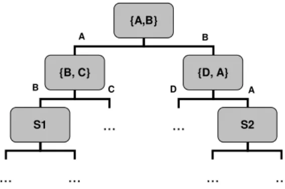
7.2 Symmetry breaking algorithms for the NValue-based model . . . 42
7.2.1 Sequential accumulation of constraints. . . 42
7.2.2 Relaxed tree accumulation of constraints. . . 42
7.2.2.1 Proof of completeness of the algorithm.. . . 43
7.2.2.2 Example. . . 44
7.2.3 Combined approach. . . 44
7.2.4 Breaking the Symmetries during search . . . 44
7.2.4.1 Pruning the domain ofX¯ . . . 44
7.2.4.2 An efficient data structure to store solutions . . . 45
7.3 Symmetry free Finite Domain model . . . 46
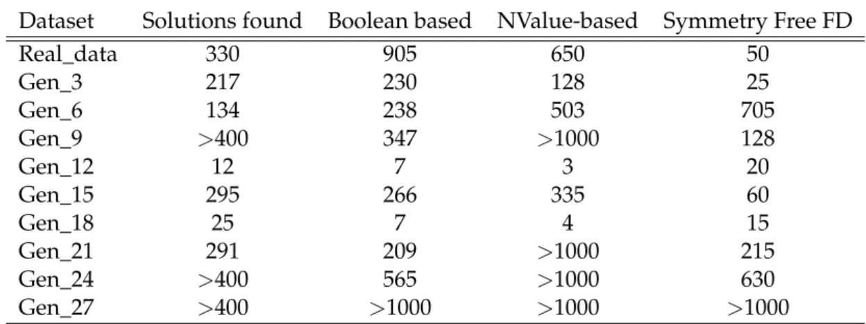
7.4 Analysis of the results . . . 47
List of Figures
2.1 Diagram of digestion . . . 4
3.1 Example of a Gomory’s cut. . . 13
4.1 An example of a CSP, the Sudoku game . . . 21
6.1 An intersection graph and its maximum independent set. . . 33
List of Tables
5.1 The datasets that will be used for testing purposes.. . . 27
5.2 Comparison between the Boolean and the Count-based models. . . 28
6.1 Comparison between the Boolean and the NValue-based models. . . 31
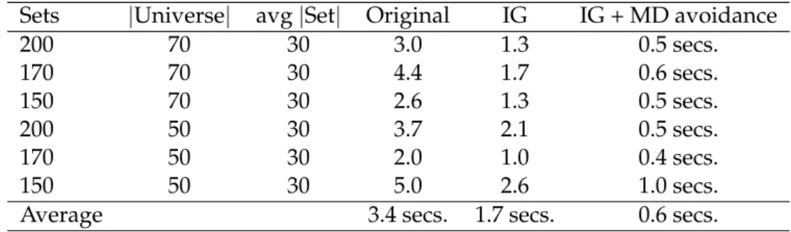
6.2 Execution time of variations of the AtMostNValue filtering algorithm. . . 38
1
Motivation
The problem of yeast identification was historically addressed through the study of both mor-phological traits and physiological features [Yar98,BPY00,BM06], but alternative molecular methods have been adopted to obtain the sequence of particular genomic regions and thus identify a given species [KR98,SFFST02].
Although sequencing nucleic acids (DNA) is more accessible than ever, it is still an sive technique, especially if applied to a high numbers of specimens. In contrast to less expen-sive techniques like RFLP, RAPD, MSP-PCR (which allow the formation of clusters among the specimens to be identified, with inherent result limitations in scope), ARDRA (Amplified Ribo-somal DNA Restriction Analysis) [VRDV+92] was proposed to differentiate between species of a eubacterial family and it represents an approach that goes beyond the mere clustering opera-tion. A fragment of the DNA of the specimen is obtained and copied many times. Enzymes are used to digest each copy, resulting in a set of fragments of DNA whose size can be meassured. Different species show different patterns of sizes for each enzyme, generally enabling the iden-tification of the organism. Variations of ARDRA [SM98,BCFA99,WBLT90] were succesfully applied to distinguish specimens among particular sets of fungal and yeast species.
However, all these approaches are based on themanualselection of enzymes such that all species that they consider can be identified.
Recent papers are acknowledging the power ofin silicocontributions in this field. One is limited to the forecast of electrophoretic patterns [PJN07], the other presents a program to as-sess the utility of a fixed set of endonucleases to distinguish between a given set of sequences [WIR+08]. However, the integration of all the available data in a comprehensive in silico ap-proach, targeting the automatic search of minimum sets of enzymes to identify the species of
1. MOTIVATION
In this disertation, the problem of finding a minimum set of restriction enzymes suitable for the task is referred to as The Species Differentiation Problem and tackled by converting it into minimum set cover and then defining a variety of Constraint Programming approaches to devise an efficient way to solve it. Furthermore the diverse techniques to solve the minimum cover are aimed to find not just one minimum set cover, but all of them.
2
Mapping the Species Differentiation
Problem into a Minimum Set Covering
problem
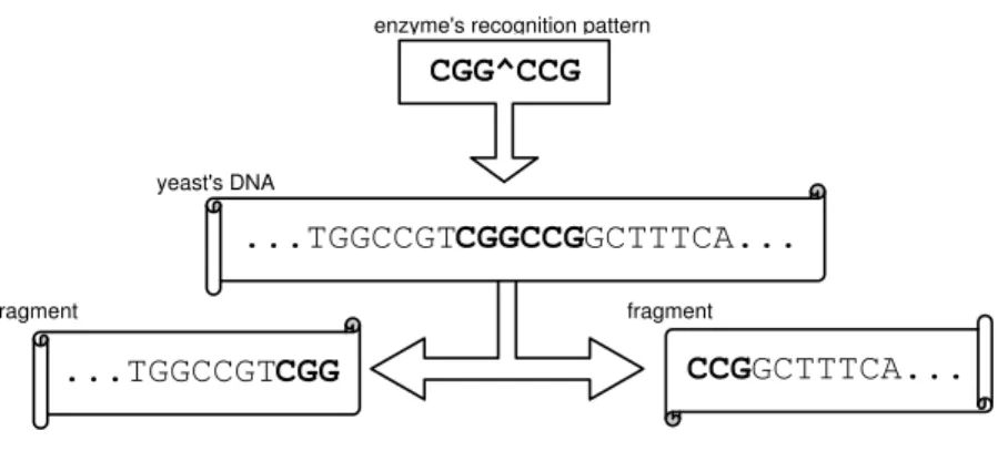
Among techniques used to identify species, ARDRA has been proposed in [VRDV+92]. This technique identifies one from a set of specimens through analysis of a specific DNA sub-sequence of its genome. Restriction enzymes (that, as is well known, cut DNA sub-sequences at specific recognition nucleotide sequences, known asrestriction sites) play a central role in the ARDRA technique that proceeds as follows: First, a “standard” fragment of the test specimen DNA is obtained (in the case of yeasts, the 5.8S-ITS region of their operons), and many copies of it are produced. Secondly, a set of restriction enzymes are separately applied to these copies. The complete digestion of each enzyme yields several smaller nucleotide segments that, subject to gel-electrophoresis, originate bands of different lengths.
2. MAPPING THESPECIESDIFFERENTIATIONPROBLEM INTO AMINIMUMSETCOVERING PROBLEM
enzyme's recognition pattern
CGG^CCG
yeast's DNA
...TGGCCGTCGGCCGGCTTTCA...
fragment
...TGGCCGTCGG
fragment
CCGGCTTTCA...
Figure 2.1: Diagram of digestion
A restriction enzymeR differentiates two yeast specimensY1 andY2if the patterns it pro-duces from them are distinguishable, i.e. at least one fragment in one of the digested yeasts is of a sufficiently different size from any fragment in the other digested yeast.
It is thus possible to produce a Boolean coverage table D, where rows denote yeast pairs (elements) and columns represent restriction enzymes (sets). In this table the cell in rowYi−Yj and columnEk denotes whether that yeast pair is differentiated (covered) by that restriction enzyme. The problem of identifying a yeast among a set of similar yeasts can be formulated as finding a setCof restriction enzymes that differentiate any pair of yeasts, i.e. for all rows there is at least one enzyme inCsuch that its corresponding column has a true value for that row.
More formally, given a set of yeastsY ={Y1, ...,YNy}and a set of enzymesE={E1, ...,ENe}, I denote asP(i,k)the induced pattern forYibyEk, i.e. the set of segment lengths produced by the digestion of yeastYiby enzymeEk. Two patternsPandQare distinct if there is a fragment length in one of them that is sufficiently different (depending on the experimental error and denoted by6≈) from any fragment of the other pattern i.e.
distinct(P,Q) =de f (∃u∈P)(∀v∈Q)(u6≈v)∨(∃u∈Q)(∀v∈P)(u6≈v)
Two yeastsYi andYj are differentiated by a restriction enzyme Ek if the patterns induced in them are distinct:
differentiate(i,j,k) =de f distinct(P(i,k),P(j,k))
A discriminating set of enzymesSis a subset of the setEof enzymes that, for any pair of yeasts in the setY, has an element that differentiates them, i.e.
2. MAPPING THESPECIESDIFFERENTIATIONPROBLEM INTO AMINIMUMSETCOVERING PROBLEM
A minimal (optimal) discriminating set of enzymesSis a discriminating set with minimal car-dinality:
min_disc(S,Y) =de f discriminate(S,Y)∧(∀R discriminate(R,Y)→#S≤#R)
Hence, given a setYof yeast specimens, the Species Differentiation Problem can be regarded as the task of finding, from a setE of available restriction enzymes, a minimal discriminating setCfor the set of yeast specimens. In set covering terms, this is translated to: given a universe U ={u1, ...,un}defined as the set of all yeast pairs, and a familyS ={S1, ...,Sn}of subsets of U representing the covering of each enzyme, find asubfamilyC ⊆S of minimum cardinality that covers all elements inU.
Although proven to be NP-Hard [Kar72], the minimum set covering problem is also a main model for several important applications such as in bus [BC96a,WR93], railway [CNS95] and airline crew scheduling, logical analysis of data [BHIK00] and location problems of facilities [MMS01].
Gel electrophoresis apparatus can analyze more than one digested sequences of DNA at the same time, but different enzymes require different environments to cut DNA sequences. Consequently, the smaller the number of enzymes required, the less costly, cumbersome and time consuming the process of specimen identification will be. This fact justifies the search of a
minimumset cover, instead of just any covering.
Not all enzymes might be available to each biochemistry lab, and the conditions required by each enzyme to function properly are different and require different facilities and apparatus. This means that the set of enzymes that one lab might regard as the best one can be very inappropriate for another for reasons that are very hard to formalize. Also some enzymes are more robust than others in the sense that they do not fail to cut DNA or can lead to the result of the gel electrophoresis experiments to be less prone to human error (J. Almeida, personal communication, January 24, 2010). This fact justifies the search forallminimum set coverings, so that the user will have as many alternatives as possible to chose from, depending on the particular conditions of the lab in which the analysis is done and their knowledge about the particular properties of each enzyme.
From now on, the work will be concentrated on the search of all minimum solutions to set covering problems through Constraint Programming, using both randomly generated data sets and real datasets obtained (during the experimental phase of this thesis) from simulations of gel electrophoresis experiments over DNA of yeast digested by enzymes.
3
Alternative approaches and state of the
art
In this section many different approaches to finding minimum set coverings are analyzed. The list is far from comprehensive, but each alternative represents one instance of a family of ap-proaches to the problem.
3.1
Population based approaches
These methods involve the existence of many individuals (each of which represent different candidate solutions) which are repeatedly processed in the search for near optimum solutions.f
3.1.1 Evolutionary Search Techniques
This kind of techniques make use of Genetic Algorithms (GAs), which are search heuristics that mimic the process of natural evolution. This search heuristic is used to generate solutions to optimization and search problems.
In a GA, the candidate solutions (calledchromosomes) are usually encoded as strings of data which represent theirgenes. The process of evolution starts from a random population of candi-date solutions from which the best candicandi-dates (as judged by afitness function) are selected and modified using diverse techniques to create the next generation of individuals. The algorithm terminates either after a fixed number of generations were produced, or a satisfactory level of fitness has been reached by an individual in the population.
3. ALTERNATIVE APPROACHES AND STATE OF THE ART 3.1. Population based approaches
Theinitial populationconsist of many individual solutions that are usually generated at ran-dom. The size of the initial population is highly problem dependent and it may vary from tens to tens of thousands. Sometimes, it is known that certain kind of individuals are near optimal solutions and in these cases this information can be used to formseedsin order to reduce the number of generations needed to achieve optimality.
Theselection stage of a GA is usually implemented by evaluating the fitness function over each individual in the population and then, by choosing elements of it that show to be better approximations to optimal solutions. To generate the next generation from that set of selected individuals, methods ascrossoverandmutationare used. The crossover genetic operator is the analogous of sexual reproduction in the biological counterpart. It mixes two chromosomes by intertwining their genes in some way. Crossover generally comes in two varieties: scattered crossoverand n-point crossover. Scattered crossover consists of the application of a particular mask to determine which genes will be taken from each parent. Inn-point crossover,npoints are defined so that sections between the points of the chromosomes of each parent are inter-leaved. Mutationconsists of the random change of bits of an individual and its purpose is to preserve and introduce diversity in the system, so to avoid local minima by preventing the homogenization of the population.
The following outline summarizes how the GA works:
1. Random creation of the initial population.
2. Creation of a sequence of new populations by:
(a) Scoring each member of the current population according to its fitness value.
(b) Scaling the raw fitness scores to normalize the values
(c) Selecting members for parenting, based on their fitness.
(d) Production of children from the parents.
• by randomly mutating a single parent or
• by combining the chromosomes of a pair of parents using crossover
(e) Replacing the current population with the children of the selected members.
3. Until the stopping criterion is met.
A very basic GA approach is taken in [DP08]. this technique is used to search for near-optimal solutions to big set covering problems. In their paper, the authors report using MAT-LAB’s Genetic Algorithm Tool and testing the method using the OR-Library [Bea90], a collec-tion of test data sets for a variety of Operacollec-tions Research (OR) problems. The set covering problems provided there contain thousands of sets and hundreds of thousands elements. The chromosomes are integer vectors X¯ = [X1, ...,Xn] which represent the list of identifiers of the selected sets. The initial population is created giving preference to the apparition of sets that cover the greatest number of elements. The selection procedure used istournament selection
3. ALTERNATIVE APPROACHES AND STATE OF THE ART 3.1. Population based approaches
reproduction phase, both crossover an mutation are used. Their experimental results show that randomly generated masks for scattered crossover worked better than 1 and 2-point crossover. The stopping criteria used was a fixed number of generations which is, obviously, a parameter very dependent on the dataset. Their basic technique fails in finding better covers for the prob-lems in the OR-Library than already known, but is presented here for introductory purposes.
In [BC96b] the chromosomes are represented as a binary vectorX¯ = [X1, ...,Xn]where the se-lection of thek−thset is expressed byXk=1. The initial population is randomly generated, as it is usually the case for this kind of algorithms. The selection phase involves dividing the pop-ulation in two pools and tournament selection is used to extract winners from each. Each pair of selected individuals is combined to form a new child solution using thefusion crossover oper-ator. This operator (originally proposed by the authors) results in the child solution to inherit more genes from the parent which is the fittest. Notably, their new mixing technique involves creating only one child from each pair of parents, while the classical cross over operators create at least two.
The children solutions generated in this manner are randomly mutated to breed the next generation of the population. This new generation does not take over the previous one, but it steadily replaces individuals which are less fit. As a consequence, the best individuals are always kept so that new comers can mate with old ones. Their approach to avoid local minima without introducing too much variation is to have a variable rate of mutation, which is indi-rectly proportional to the speed at which the populations genetically converge. This technique has the consequence that the dominating factor governing the direction of search changes with time. At first, when the population is highly diverse, the crossover operator dominates the search but as the evolution process advances it is mutation what stands over.
When new solutions are born, they are first corrected to close feasible solutions using greedy heuristics by the so calledrepairoperator. Also their genome is cleaned from redun-dant genes (which represent sets that can be discarded without loosing the covering properties of the solution) as a way of maintaining solutions as small as possible.
This implementation depends on many parameters that have to be manually set. Some can be deduced from the properties of the dataset in analysis but others can not be known and it is the tester who tries different combinations and try to find the best ones. They report obtaining good results over the datasets in the OR-Library, some times finding solutions of smaller cardinalities than previously known, and other times failing to compete with other approaches.
3. ALTERNATIVE APPROACHES AND STATE OF THE ART 3.1. Population based approaches
The initial population is created so that for each gene, the sets that cover it have an equal probability of being chosen. The fitness function is defined in terms of thecostof the covering, which is reduced to the number of sets used when unicost set covering is considered. The selection operator in their GA implementation is probabilistic in the sense that it is more likely to choose more fit individuals. For mixing parent individuals they use a special purpose LP-crossoverbased in a relaxation of a Linear Integer Program solved through the Simplex method, what aims to find a good combination of the parent genes. The mutation procedure chooses gens at random and changes them also in a random fashion but giving higher probabilities to set identifiers of smaller cost (which becomes a uniform distribution in unicost set covering).
When they apply their GA to the OR-Library, they obtained very similar results to the pure Linear Programming (LP) approaches that will be presented later, meaning that the coverings found were almost always the same size as those found with the LP approaches. The execution time of their algorithm was some times above and some times under the other LP implemen-tations, what does not allow much generalization about the efficiency of it.
Any evolutionary approach to set covering is bound to find only near-optimum solutions because it does not intend to prove that a better solution is not possible.
3.1.2 Ant Colony Optimization
The ant colony optimization algorithm (ACO) is a probabilistic technique for solving computa-tional problems by reducing them to the search of good paths through graphs. Artificial ants in ACO algorithms can be seen as heuristics that iteratively generate solutions by taking into ac-count search experiences accumulated in the past. These past experiences are modeled through
pheromone trails
Biologists have observed that ants tend to find the shortest path between their colony and a source of food, what means that imitating their individual behavior might be useful. A way of modeling this individual behavior is:
1. An ant initially wonders randomly around the colony.
2. When it discovers a food source it returns directly to the nest, leaving in its path a trail of pheromone
3. These pheromones are attractive to other ants, which will be inclined to follow the track.
4. While returning to the colony after finding food at the end of that path, these ants will strengthen the pheromone trail.
5. It is usually the case that there are more than one single route to reach the same food source, but after a while the shorter one will be traveled by more ants than the other one.
6. The shortest route will be increasingly enhanced, becoming more attractive on each iter-ation.
3. ALTERNATIVE APPROACHES AND STATE OF THE ART 3.1. Population based approaches
8. After a while all the ants will be following the same short route, meaning that they will have found a good solution to the problem.
ACO algorithms have been applied to the Set Covering Problem. For example in [SH00] an ant starts with an empty solution and constructs a complete one by adding sets until are elements are covered. Each set identifier jhas a associated a pheromone trailτj, and a heuristic valueηj.τj indicates the learneddesirabilityof including the set jin the solution of an ant and ηj indicates a different desirability value obtained by other means, such as the proportion of still uncovered elements that set jwill cover if selected. The pheromone trails are updated after a fixed numbermaof solutions were constructed and improved by local search. The ants prefer selecting sets with high associated pheromone trail and/or heuristic value.
The algorithm outline for ACO applied to the Set Covering Problem is shown in Algorithm 1.
Algorithm 1Ant Colony Optimization for the Set Covering Problem 1: while¬termination conditiondo
2: for allk∈ {1, ...,ma}do
3: whilesolution not completedo 4: applyConstructionStep(k)
5: end while
6: eliminateRedundantColumns(k) 7: optimizeThroughLocalSearch(k) 8: end for
9: updateStatistics 10: update Pheromones
11: end whilereturnbest solution found
In theMAX-MINAnt System proposed in [SH00], solutions are constructed by setting the probability of choosing each set for each ant. An antkchooses set jwith probability
pkj=
τj(ηj)β ∑ g∈/Sk
τh(η)β , if j∈/Sk 0 , otherwise
where the parameterβ >0sets the relative influence of heuristic against pheromone informa-tion. Sk is the partial solution achieved by thekth ant. After all solutions are computed, the pheromone trails have to be updated by first evaporating them (updatingτj to (1−ρ)τj, ∀j) and then adding an amount∆τ =1/z to the sets contained in the best solution found so far, wherezis the cost of the solution used in the pheromone update (which in unicost set covering is the number of sets in the cover). When no new improved solution is found for a given num-ber of iterations, the pheromone trails are re-initialized as a way to reset the search and avoid local minima.
3. ALTERNATIVE APPROACHES AND STATE OF THE ART 3.2. Linear Programming approach
of the search space.
In the paper it is reported that when compared to other algorithms, ACO approaches can reach state-of-the-art performance on various instances, but are not as powerful or robust as those based in Linear Programming. Moreover, ACO approaches are highly dependent in the manual setting of various parameters such asβ andma.
3.2
Linear Programming approach
Linear programming (LP) constitutes a very important technique for the optimization of a lin-ear objective function, subject to linlin-ear equality and inequality constraints. This method is used in many areas, one of it being business and economics due to the fact that problems like maximizing outcome can be straightforwardly stated and efficiently solved.
3.2.1 Linear Programs
In their canonical form, linear programs are expressed as:
maximize/minimize c⊤x subject to Ax≤b
where x is a vector of variables whose values must be determined, c and b are vectors of known coefficients andAis a matrix of known coefficients. The expressionc⊤xis to be maxi-mized/minimized within the limits defined byAx≤b.
As an example, suppose that a farmer owns a land of A square kilometers and wants to plant a combination of wheat and barley. The farm has a limited amountF of fertilizer and Ppesticide, which are resources required by both crops in different amounts per unit of area. Wheat requiresF1 units of fertilizer andP1of pesticide, but barley needsF2 andP2 per unit of area. Let the selling prices of wheat and barley beS1 andS2 respectively. By denoting with x1andx2 the areas planted of each crop, the problem of finding the optimal number of square kilometers to plant each crop can be expressed as the linear programming problem:
maximize S1x1+S2x2 subject to x1+x2≤A
F1x1+F2x2≤F
P1x1+P2x2≤P
x1≥0
x2≥0
In this simple problem using only two variables, the space search can be represented as a plane. Each of the constraints are actually linear functions that cross the plane delimiting the area of
3. ALTERNATIVE APPROACHES AND STATE OF THE ART 3.2. Linear Programming approach
Linear programming problems can be solved using different very well known methods such asSimplex[NM65],ellipsoid[GLS81] andInterior Point[Gli99].
Simplex is very efficient in practice, although exponential in the worst case. It takes advan-tage of the fact that solutions that maximize/minimize the objective function are present in the intersection between constraints and, using mathematical machinery, it visits the corners of the feasible solutions space in an order that guarantees better approximations on each iteration. This way the algorithm can assure that once a local maximum/minimum is found, it is also a global maximum/minimum. Alternative methods such asEllipsoidand variations of Simplex [Kel06] show that Linear Programing is solvable in polynomial time, but these methods are too inefficient in practice to be of much practical use.
Oppositely to Simplex, Interior Point methods reach an optimal solution by traversing the interior of the feasible region. These methods are characterized by the use of continuously parametrized families of approximate solutions that asymptotically converge to the optimum solution. These paths trace smooth trajectories with algebraic properties that can be exploited by the algorithms.
3.2.2 Integer Linear Programming
Consider the manufacture of computers. A linear programming model might give a production plan of 130.6 computers per week. In such a model, it is a fairly reasonable assumption that 130 computers per week would be pretty close to optimality. On the other hand, suppose a com-pany is building roads. Then a model that suggests that 0.8 roads should be built connecting some pair of cities and another 0.4 roads should be finished for other pairs of locations would be of little to no value. Roads come in integer quantities, and that fact should be considered by the models.
At first sight, this restriction of integrality may seem innocuous, but in reality it has far reaching effects. With integer variables, a whole new family of problems can be addressed, but the computation of optimum solutions becomes much more costly.
3.2.2.1 Cutting planes
Although solving linear programs with integer coefficients is an NP-hard problem, a relax-ation of the integer condition permits a relatively efficient search for integer solutions when combined withCutting Planetechniques.
3. ALTERNATIVE APPROACHES AND STATE OF THE ART 3.2. Linear Programming approach
case the problem still takes exponential time to be solved, but in practice the approach works efficiently enough to make it applicable to a broad range of problems.
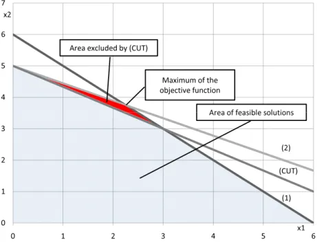
To exemplify the concept of Gomory’s cut consider this tiny Integer Linear Program prob-lem:
maximize 5x1+8x2 subject to x1+x2≤6 (1)
5x1+9x2≤45 (2)
x1≥0
x2≥0
x1,x2integers
The relaxation of the problem can be plotted in a plane. In Figure3.1the constraints(1)and (2)are represented by lines and the point that maximizes the objective function is marked with a label. The non integer of the problem isx1=2.25andx2=3.75and it is used to create the Go-mory’s cut labeled as(cut), which represents the additional constraint2/3x1+x2≤5. Note how this cut does not prune any integer solution from the search space (shadowed) but effectively removes the previous solution from it. The process can be repeated iteratively adding new cuts until an integer solution is found.
4 5 6 7
Maximum of the objective function
Area of feasible solutions Area excluded by (CUT)
x2
0 1 2 3
(2) (CUT)
(1) Area of feasible solutions
x1 0 1 2 3 4 5 6
x1
3. ALTERNATIVE APPROACHES AND STATE OF THE ART 3.2. Linear Programming approach
3.2.2.2 Branch and Bound
Branch and Bound techniques work rather differently than cutting planes. They consist in di-viding the search space by choosing a variable andbranchingover, creating different linear pro-grams, each of which has a different value fixed for that variable. Abounding functionestimates the best value of the objective function obtainable in each branch in an optimistic manner, and the Branch and Bound algorithm visits first the nodes predicted to give better solutions. As so-lutions are found, all branches pending to be solved whose bounding function predicts worst results than the best solution known can be safely discarded. Thispruningmechanism will not cut any potentially good branch since the bounding function is an optimistic one, meaning that the value predicted by it will be always better or equal than the objective function applied to the best solution in that branch.
The most delicate part in the use of Branch and Bound techniques is finding a tight bound-ing function. The computation of the boundbound-ing function often consist of solvbound-ing the Lagrangian dual of the original problem. The original formulation of the LP is called theprimalproblem and the dual consist of a transformation which, when solved, provides an upper bound to the optimal value of the primal problem. This transformation has the property that the dual of a dual linear program is the original primal program. By using the dual of a problem in a branch, one can therefore predict a bound on how good solutions in that branch will be and then decide if the branch is to be discarded or not.
3.2.3 Lagrangian Relaxation
The Lagrangian relaxation is even softer than the linear relaxation and it is used to find near-feasible solutions in an efficient manner. It works by moving the constraints into the objective function so as to consider their lack of satisfaction as a penalty. The Lagrangian dual of a Integer Linear Program is often solved throughsubgradient optimization. These problems frequently involve an objective function which is not differentiable in all points of its domain. Assuming the objective function is to be maximized, this means that in those points, the direction of highest gradient (in which the objective function will increase the most) can not be computed by using the derivate of the objective function, since it does not exist. On the other hand, it is possible to use the concept ofsubderivativeof the function in a point, which is a slope such that if a line with that slope passes through that point, it is everywhere either touching or below the function but it never crosses through it. The subgradient optimization method takes advantage of this concept and uses it to compute a subgradient of the objective function in the points in which it is not differentiable. This subgradient will point in a direction that will make the objective function increase, and by iteratively following that path, the subgradient optimization method travels though the search space in a direction that maximizes the objective function.
It should be noted that at any non differentiable point of a function, there are an infinite number of subgradients, and it is generally not possible to find the one for which the objective function increases the most.
3. ALTERNATIVE APPROACHES AND STATE OF THE ART 3.2. Linear Programming approach
but just as a heuristic to find near optimum solutions.
3.2.4 Integer Linear Programming formulation of the minimum set covering
prob-lem
Given the coverage tableDa booleanm×nmatrix, whereM={1, ...,m},N={1, ...,n}, a column j∈N is said to cover a row i∈M if Di j=1. The minimum set covering problem calls for a minimum subsetS∈Nof columns such that each rowi∈Mis covered by at least one column
j∈S. The Integer Linear Programing definition of the problem is then:
minimize
∑
j∈Nxj
subject to
∑
j∈NDi jxi≥1 i∈M
xj∈ {0,1} j∈N
wherexj=1iff j∈S.
As it was said above, the relaxation of the last constraint to0≤xj≤1, transforms the prob-lem into a non-integer version. This allows much more efficient computation ofnearsolutions by allowing instances in which sets are not selected nor discarded. In conjunction with Gomory cuts this technique is able to findproper minimum covers in a very efficiently manner. Alter-native to the cutting plane techinques, Branch and Bound techniques often use Lagrangian relaxations to solve the dual problem through subgradient optimization methods to provide bounding functions.
The algorithm proposed in [Bea87] uses the Branch and Bound method and the lower bounds are computed using the Lagrangian relaxation together with subgradient optimization. The relaxation of integer problems in the branches are solved to optimality by the dual simplex method. Several dominance procedures to reduce both the number of rows and columns are applied. These dominance procedures basically eliminate columns which cover a subset of rows with respect to other columns, and elements which are covered by a superset of columns with respect to others. Instances of up to 400 rows and 4000 columns are tackled, finding cov-erings of minimum cardinality.
3. ALTERNATIVE APPROACHES AND STATE OF THE ART 3.3. Local Search strategies
the other LP implementations.
In [LNF95] a different heuristic based on continuous surrogate relaxations and subgradient optimization is presented. Since their approach does not use either Branch and Bound nor cutting planes, the method is also aimed at huge set covering problems for which near-optimal solutions are deemed acceptable. The surrogate relaxations are created by combining many constraints into one single (less strict) constraint, with the expectation that the simpler system might also mantain some collective property of the constraints. The subgradient optimization method is used to guide the search in the direction of better solutions. Their algorithms applied to the datasets in the OR-Library showed it to be very competitive, finding better solutions than previously known for a couple of instances.
The field of Linear Programming techniques to solve set covering problems is very deep and there exist a wide variety of heuristics, relaxations and transformations to fine tune the search for different kinds of datasets. In this regard, what is important to note is that the main empha-sis is put into developing strategies to cope with very large datasets for problems in which only one near-optimal solution is required. This fact makes most of them inappropriate to solve the enzymes problem, where the aim is to find all truly minimum coverings. Techniques like cut-ting planes and Branch and Bound can be used to find true minimum set coverings and might be applicable to the datasets which are dealt with in this dissertation. However, the addition of non linear constraints (as proposed in the Further Work section of the present thesis) would also make them inappropriate to solve the arising problem.
3.3
Local Search strategies
Local search consists of a metaheuristic used to solve computationally hard optimization prob-lems. It can be applied when the problems are formulated as the search for a solution that maximizes a criterion among a number of candidate solutions.
This kind of algorithms traverse the search space by iteratively moving from candidate so-lution to candidate soso-lution following a path through theneighborhood relation, until a solution deemed good enough is found, or a time bound is elapsed. Usually every candidate has more than one neighbor solution and the choice between them is made with the aid of information about the neighborhood (hence the namelocal) and previous experience.
Typically a set of constraints that an appropriate solution should satisfy is defined and, even though candidate solutions that violate the constraints are permitted, the number of satisfied constraints is used as part of the maximization criterion.
3. ALTERNATIVE APPROACHES AND STATE OF THE ART 3.4. Greedy algorithm
To guide the search, a fitness function is defined to be the sum of the size of the solution and the number of elements that it leaves uncovered. This function is not computed from scratch each time, but it is updated from previous computations of it.
The initial solution is created using a greedy algorithm that starts with an empty solution and iteratively adds the sets which cover most still uncovered elements. Cycles in the search are avoided through atabulist (of a size related to the size of a solution obtained by the greedy algorithm) that temporarily forbids adding/removing sets recently deleted/added.
The stopping criteria used is based on bounding the number of times that the moves can be applied without improving upon the best solution found so far.
This very simple method is cited with introductory purposes, and it is not very competitive with respect to other more involved approaches as the one presented next.
In [YKI03] the solutions are not defined as the list of selected set identifiers but rather as the binary vectorX¯ ={X1, ...,Xn}, where the selection of thek−thset is represented byXk=1. The neighbor relation is not defined by erasing, adding or replacing sets one at a time, but by switching many elements ofX¯ at once. Ther-flip neighborhood of a solutionX¯ ={X1, ...,Xn}is the set of solutions obtainable by flipping at mostrelements ofX¯. The size of such a neighbor-hood isO(nr)but they propose an implementation based on a Linear Program with Lagrangian relaxations to reduce the number of candidates in the neighborhood without sacrificing solu-tion quality. Their experimental results showed thatr=3gives a very good trade off between the size of the neighborhood and the speed of convergence to near-optimality.
A strategic oscillation mechanism is used to travel through the search space alternating be-tween feasible and infeasible solutions. This technique is used as a way to avoid local minima. Following a path through the frontier is justified by the intuitive fact that changing very little in minimum solutions will result in uncovered elements, what means that minimum solutions must be in the edge of feasibility.
Local search is alternated with variable fixing. This trick also uses a Lagrangian heuristic so that the sets considered as best by it are selected, and those which are considered worse are automatically discarded.
The objective function is defined to be the number of elements not covered (or the sum of their costs in the weighted version) together with a penalty that is used to avoid cycles. Their stop criterion is a fixed number of iterations without finding better solutions to the best known so far.
This sophisticated method is reported to be very robust and efficient, winning also over many Linear Programing approaches in some instances of the OR-Library.
3.4
Greedy algorithm
3. ALTERNATIVE APPROACHES AND STATE OF THE ART 3.5. Backtrack algorithm
Algorithm 2Greedy algorithm Input:
—U ={u1, ...,un}, the universe of elements —S ={S1, ...,Sm}, the family of subsets ofU Output:
—Ca cover of low cardinality 1: C← /0
2: U←U
3: whileU6=/0do 4: s←argmax
k∈S
|k∩U| ⊲select the most covering set with respect to the still uncovered elements
5: C←C∪ {s} ⊲the selected set is added to the cover family
6: U←U\s ⊲the covered elements are removed
7: end while
The pseudo code is shown in Algorithm2.
Of course, this greedy approach does not guarantee that, upon termination, a minimum cover will be found. In fact, notwithstanding the very fast execution time of the algorithm, the solutions found with the benchmark datasets that will be presented latter were never min-imum. However, this algorithm can be used in the minimization process to establish a first upper bound for the size of the minimum cover.
3.5
Backtrack algorithm
This kind of algorithms guarantees optimality by searching almost over the whole search space. After first solution is found, it can prune all possibilities that make use of worse solutions. The way in which this approach travels through the search space slightly resembles Constraint Pro-gramming approaches, introduced in the next chapter. The pseudo code is shown in Algorithm 3.
This approach involves searching blindly for a complete coverage of the universe. All exact algorithms are bound to be exponential in complexity since minimum set covering is NP-hard, but as this algorithm makes no inference about the consequences of choosing one set over another, it is a very inefficient one.
3.6
Conclusions
3. ALTERNATIVE APPROACHES AND STATE OF THE ART 3.6. Conclusions
Algorithm 3Backtrack algorithm Input:
—U ={u1, ...,un}, the universe of elements —S ={S1, ...,Sm}, the family of subsets ofU Output:
— Solve(/0,S,S) returns a cover of minimum cardinality
Procedure Solve(S,R,Best) ⊲S: selected sets,R: available sets,Best: best covering found
1: if|S| ≥ |Best|then
2: returnBest
3: else ifScoversU then
4: returnS
5: else
6: R← {s} ∪R′ ⊲selectsnon deterministically
7: S′←S∪ {s}
8: S1=Solve(S′,R′,Best) ⊲binary choice
9: S2←Solve(S,R,S1)
10: returnS2
11: end if
End Procedure
4
Background on CSP
In this chapter the main aspects of Constraint Satisfaction Problems are reviewed to provide the framework of the models proposed in following chapters.
4.1
Constraint Satisfaction Problems
Constraint satisfaction problems (CSPs) are mathematical problems whose definition includes a set of objects whose state must satisfy a number of constraints. These constraints are basi-cally limitations that state relations between the objects that must be preserved. Objects are represented as homogeneous variables whose state is the value that they are assigned to.
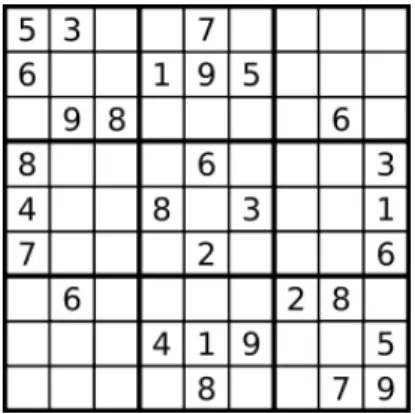
As a simple and representative example of a CSP let us take the case of the very well known game Sudoku. This game consists of a table of9×9cells divided in sections of3×3as shown in Figure4.1. Each cell in the table can be assigned to numbers from1to9and some of the cells come already labeled. The rules of the game state that there cannot be repeated numbers in any row, column or3×3section. In the CSP of Sudoku, there are9×9variables whose domains are numbers in the range1..9and the constraints simply state the rules of the game, namely that all the variables in a row, a column or a section must be different from each other. Apart from how easy it is to define the problem in this manner, the advantage of using this approach is that there are very efficient algorithms for filtering the allowed values for each variable given a partial labeling of them.
More formallya CSP is a triplet<X¯,D¯,C >, where
• X¯ ={X1, ...,Xn}is a set of variables.
4. BACKGROUND ONCSP 4.2. Propagation
Figure 4.1: An example of a CSP, the Sudoku game
say thedomainsof the variables.
• C is the finite set of constraints imposed overX¯.
A constraintCin the set of constraintsC over the set of variablesvar(C) = (Xi
1, ...,Xir)is a subsetrel(C)of the Cartesian productD(Xi1)×...×D(Xir)that specifies theallowedcombinations of values for the variablesXi1, ...,Xir.
Given a subsetY¯ of the variables inX¯, aninstantiation I ofY¯ is an assignment of values to variables such that∀X∈Y¯, the valueaassigned toXbelongs toD(X). An instantiationIsatisfies a constraintCif and only if the projection ofI onvar(C)belongs torel(C). IfI does not satisfy the constraintC, then it is said thatIviolatesit.
Cisconsistentif and only if there exists a tuple ofrel(C)which is valid. A valuea∈D(X)is
consistentwithCif and only ifX∈/var(C)or there exists a valid tuple ofrel(C)in whichais the value assigned toX.
The Constraint Satisfaction Problem(CSP) consist of finding a full instantiation I ofX¯ such that∀C∈C,IsatisfiesC.
4.2
Propagation
Constraint solvers typically explore partial instantiations enforcing a local consistency property using specialized and general purpose propagation algorithms. Local consistency requires that all consistent partial instantiations can be extended to another variable in such a way that the resulting assignment is consistent. Local consistency properties can be grouped into various classes depending on how strict they are. The main classes of local consistency are node, arc and path consistency.
Node consistencyrequires that all unary constraints on a variable are satisfied by each of the values in its domain. This condition can be enforced by simply reducing the domain of each variable to that which satisfies all unary constraints on the variable.
The case ofarc consistencyis slightly more complicated. Given a constraintCon the variables ¯
4. BACKGROUND ONCSP 4.3. Unary, binary and global constraints
consistent withYi =vj with respect toC. If all values inYi have support,Yi is said to be arc consistent. The variableYiisgeneralized arc consistent(GAC) onCif and only if every value in D(Yi)has support onC. A constraintCis said to be GAC if and only if each constrained variable is GAC onC. Enforcing GAC requires eliminating all the values from each variable that do not have support.
Path consistencyis similar to arc consistency but it requires pairs of variables to have sup-port. A pair of variables is path consistent with respect to a third variable if any arc consistent assignment of the pair of variables has support on the third one. This kind of consistency is usually not enforced by solvers since its complexity is generally not justified by its pruning power.
Constraint propagation then proceeds by enforcing node and arc consistency over all the variables, effectively reducing the search space without eliminating any solution that satisfies the constraints.
4.3
Unary, binary and global constraints
Constraints are classified depending on the number of variables that they relate. Unary con-straints involve only one variable and its domain can be reduced simply by enforcing node consistency over it. Binary constraints state relations between pairs of variables, and their prop-agation involves enforcing arc consistency. Constraints that involve more than two variables are regarded asglobal constraints. For this class of constraints it might be possible to enforce path consistency, but for efficiency reasons the more relaxed approach of enforcing generalized are consistency is used. Specialized algorithms for enforcing GAC in many global constraints exist, and they work by analyzing underlying properties of the system that have to be verified. A prominent case of a global constraint is that of AllDifferent [R´94], in which bipartite graph theory is used to enforce GAC in polynomial time. This constraint is equivalent to stating in-equality constraints between each pair of variables, but this simplistic approach misses some properties than can only be exploited when all variables are considered together. The most ef-ficient filtering algorithms for this constraint build a bipartite graph containing the variables in one partition and the set of values in the other, and proceeds by pruning values from variables that do not belong to any maximum matching of the bipartite graph. In following sections the case of theNValueglobal constraint will be analyzed in detail.
4.4
The importance of finding the right model for a constraint
satis-faction problem
4. BACKGROUND ONCSP 4.5. Minimization
Furthermore sometimes a set of constraints define the problem completely, but the specifica-tion of addispecifica-tionalredundantconstraints accelerates the process of finding solutions by allowing the application of more pruning algorithms.
Other times the problems are required to be solved in steps being the set of constraints applied on each step complementary to those on the previous one. First a CSP is solved to find the parameters to build another CSP. This is the case of finding all minimum solutions to set covering problems studied in this dissertation. First the size of a minimum cover is found using a model that is efficient for that task, and then another model (some times similar to the previous one) is used to find all solutions knowing already their cardinality.
4.5
Minimization
Constraint satisfaction problems are also used to find optimal solutions of various optimiza-tion problems. In this family of problems constraints are used to specify the properties that a solution must satisfy. The interest is put not in any valid solution but only in those which minimize an objective function defined over the elements of the candidate solutions.
The main method used in this kind of problems is Branch and Bound (BB). The Branch and Bound procedure is an intelligently structured search over the search space. The space of all feasible solutions (that which satisfy the constraints) is partitioned repeatedly into increasingly smaller subsets and an upper bound is calculated for the objective function of the solutions that fall in each subset. After each partitioning, those subsets with a bound that is greater than that of a known solution are excluded from the search. The partitioning proceeds until a solution is found such that the objective function applied to it results in a value which is smaller than the bound for any subset.
In the case of minimum set covering, the objective function gives a lower bound on the size of the candidate solution. Whenever a branch can be predicted to use more sets than the best solution found so far (by means of the objective function), the BB method will automatically discard it.
In Constraint Programming the objective function is actually represented as a variable, called objective variable. A set of constraints are imposed that relate it with the other vari-ables in the problem, so that it reflects the objective function. As the BB method explores a branch, the domain of the objective variable is pruned by the enforcement of the local consis-tency property, what effectively gives bounds to the objective variable, allowing the BB method to know when a branch can be discarded.
5
Minimum set covering models
Two different methods to solve the problem of finding the size of a minimum cover are pre-sented here. Their implementation was done in Sictus Prolog and shred some light into the subtleties of minimum coverings.
5.1
Boolean variables model
This model is easier to define in terms of a coverage matrix representation. GivenDanm×n matrix, whereM={1, ...,m},N={1, ...,n}, a column j∈Nis said tocovera rowi∈MifDi j=1.
A Vector of boolean variablesX¯ ={X1, ...,Xn}is created were the selection of the jthset in the covering is modeled byXj=1. A Constraint Programming system simply solves the problem of finding an assignment ofX¯ such that the selection of sets covers all the universe. The covering of thejthelement is represented the assertion∑nj=1XjDi j≥1. By minimizing the sum ofX¯ while labeling it, the minimum solution can be found rather efficiently. The pseudo code is shown in Algorithm4. This model performs very well in practice since the propagation of constraints drastically prunes the space search of the vectorX¯.
5.2
Count-based Finite Domain model
VectorC¯ is defined having a size fixed on an upper bound of the cardinality of a minimum cover (this upper bound can be computed using the simple greedy algorithm).
Set constraints are imposed over the variables in the vector stating that for each element of U it is the case that at least one set identified inC¯contains it. This means that after labeling,C¯
5. MINIMUM SET COVERING MODELS 5.3. Benchmarks
Algorithm 4Boolean CP model Input:
—D, anm×nmatrix Output:
—X¯ a vector representing a selection of sets that constitute a cover of minimum cardinality
1: X¯ ←[X1, ...,Xn] ⊲There is one boolean variable for set inS
2: for all j∈1..ndo 3: Xj∈0..1 4: end for
5: for alli∈1..mdo
6: ∑nj=1XjDi j ≥1 ⊲The cover of each element is imposed as a constraint
7: end for
8: label(X¯): minimizing ∑ j∈1..n
Xj
!
The search for a minimum solution is done by adding one extra value /0 to the domain of the variables ofC¯that represents a null selection. By labelingC¯while maximizing the count of /0 elements, the number of selected sets is minimized, and the result is a minimum set cover. The variables ofC¯are constrained to follow a strict ordering, and an extra limitation is imposed to assure that the non null selections will be present all together at the beginning of the vector; this way the apparition of symmetries is avoided. The pseudo code is shown in Algorithm5.
Algorithm 5Finite Domain Count-based model Input:
—U ={u1, ...,un}, the universe of elements —S ={S1, ...,Sm}, the family of subsets ofU
—N, an upper bound on the cardinality of a minimum set covering Output:
—Ca cover of minimum cardinality 1: C¯= [C1, ...,CN]
2: for alli∈1..N−1do
3: Ci<Ci+1∨Ci+1=/0 ⊲symmetries are broken by imposing a strict ordering
4: Ci=/0⇒Ci+1=/0 ⊲and by forbidding sets after the first/0
5: end for
6: for allu∈U do
7: E← {S:S∈S,ui∈S} ⊲Erepresents all sets that cover the elementui
8: W
i∈1..N
Ci∈E ⊲a disjunctive constraint is imposed to assure total covering
9: end for
10: Count(C¯,/0,M)
11: label(C¯): maximizing(M)
5.3
Benchmarks
5. MINIMUM SET COVERING MODELS 5.3. Benchmarks
The intended area of application of these methods is that of relatively small set covering prob-lems with particular properties arising from the patterns obtained from gel electrophoresis experiments applied to digested fragments of DNA. As it is stated in the motivation section, this is useful to enable low cost identification of species in a family of physically very similar organisms.
One dataset was constructed using real data about the Species Differentiation Problem and it is labeled asReal_data. The enzymes were applied to the DNA of each yeast species and then gel electrophoresis simulations were computed to find the patterns that each combination of enzyme - yeast would produce. This patterns are compared to find the yeast pairs that each enzyme is capable of differentiate.
However, since the information necessary to build more datasets for benchmarking pur-poses is not easily available, the only alternative is to study the properties of the original prob-lem and use that information to artificially build new different coverage tables.
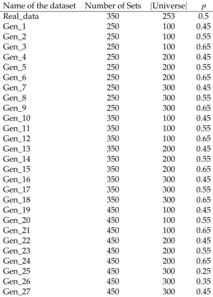
It only takes one digested DNA fragment to be of a different size in two species to make them distinguishable through the enzyme with which it was digested, so in spite of the fact that physically similar organisms typically share recent common ancestors (what makes their DNA to be similar), enzymes have an outstanding capacity for differentiating them. The consequence of this is that each enzyme will cover a considerable percentage of the total numbers of yeast pairs. In the context of set covering (and using the real dataset as reference), this means that when generating random datasets the probability p that a set will cover any given element should be high. In turn, this fact results in very dense coverage tables. Here (with the exception of datasets Gen_25 and Gen_26) values forpbetween45%and65%are considered:
0.45≤p≤0.65
Moreover, the typical number of species in this kind of analysis is not large [VRDV+92], and here between 15 and 25 species will be assumed. The number of different species pairs that can be constructed formndifferent species isn∗(n−1)/2, resulting in a universe of a size between100and300:
100≤ |U niverse| ≤300
Finally the total number of commercially available enzymes is350but for testing purposes, the total number of sets in the family will be considered to be between 250 and 450.
250≤Sets≤450
These parameters are somewhat arbitrary, but are based upon the analysis of the problem which the generated datasets intend to represent, and the assumption that the information gathered from real enzymes and yeast species is representative.
5. MINIMUM SET COVERING MODELS 5.4. Results
Name of the dataset Number of Sets |Universe| p
Real_data 350 253 0.5
Gen_1 250 100 0.45
Gen_2 250 100 0.55
Gen_3 250 100 0.65
Gen_4 250 200 0.45
Gen_5 250 200 0.55
Gen_6 250 200 0.65
Gen_7 250 300 0.45
Gen_8 250 300 0.55
Gen_9 250 300 0.65
Gen_10 350 100 0.45
Gen_11 350 100 0.55
Gen_12 350 100 0.65
Gen_13 350 200 0.45
Gen_14 350 200 0.55
Gen_15 350 200 0.65
Gen_16 350 300 0.45
Gen_17 350 300 0.55
Gen_18 350 300 0.65
Gen_19 450 100 0.45
Gen_20 450 100 0.55
Gen_21 450 100 0.65
Gen_22 450 200 0.45
Gen_23 450 200 0.55
Gen_24 450 200 0.65
Gen_25 450 300 0.25
Gen_26 450 300 0.35
Gen_27 450 300 0.45
Table 5.1: The datasets that will be used for testing purposes.
enzymes and the other 27 were randomly generated using the parameters stated in each line.
5.4
Results
5. MINIMUM SET COVERING MODELS 5.4. Results
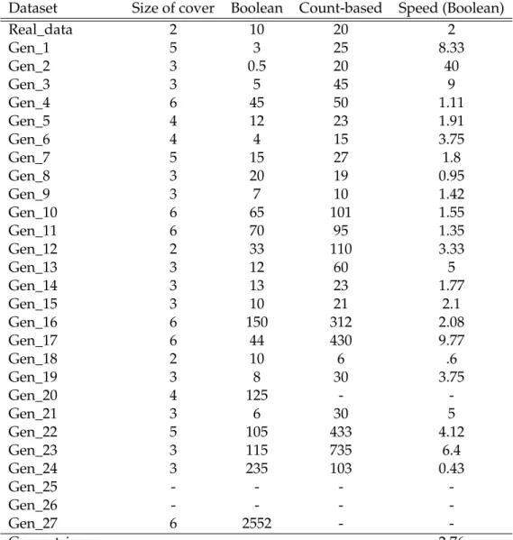
Dataset Size of cover Boolean Count-based Speed (Boolean)
Real_data 2 10 20 2
Gen_1 5 3 25 8.33
Gen_2 3 0.5 20 40
Gen_3 3 5 45 9
Gen_4 6 45 50 1.11
Gen_5 4 12 23 1.91
Gen_6 4 4 15 3.75
Gen_7 5 15 27 1.8
Gen_8 3 20 19 0.95
Gen_9 3 7 10 1.42
Gen_10 6 65 101 1.55
Gen_11 6 70 95 1.35
Gen_12 2 33 110 3.33
Gen_13 3 12 60 5
Gen_14 3 13 23 1.77
Gen_15 3 10 21 2.1
Gen_16 6 150 312 2.08
Gen_17 6 44 430 9.77
Gen_18 2 10 6 .6
Gen_19 3 8 30 3.75
Gen_20 4 125 -
-Gen_21 3 6 30 5
Gen_22 5 105 433 4.12
Gen_23 3 115 735 6.4
Gen_24 3 235 103 0.43
Gen_25 - - -
-Gen_26 - - -
-Gen_27 6 2552 -
-Geometric mean 2.76
6
A new minimizing NValue-Based
model
The failure of the minimizing Count-Based model presented in the previous section motivated further analysis of the problem. This resulted in a very efficient model based in the NValue global constraint which is capable of finding the size of a minimum cover in record time.
6.1
NValue-based Finite Domain model
This model is somewhat the dual of the boolean model. Instead of finding a solution through the labeling of a vector that has as many elements as the cardinality ofS, this approach in-volves a vector with one variable for each element inU
Now each variableXi in theX¯ vector is associated to the elementuiin the universe, and its domain is the set of identifiers of subsets in the familyS that cover such element. By labelingX¯ while minimizing the number of different values that it makes use of, minimum set coverings are found. The pseudo code is shown in Algorithm6.
6. ANEW MINIMIZINGNVALUE-BASED MODEL 6.2. Results
Algorithm 6NValue-based Finite Domain model Input:
—U ={u1, ...,un}, the universe of elements —S ={S1, ...,Sm}, the family of subsets ofU Output:
—Ca cover of minimum cardinality
1: X¯ = [X1, ...,X|U|] ⊲one Finite Domain variable for each element inU
2: list_to_set(X¯,C)
3: for alli∈1..|U|do
4: Xi∈ {k∈1..|F|:uk∈Si} ⊲the domain ofXiis the set of set identifiers inF that cover theith element ofU
5: end for
6: label(X¯): minimizing(|C|)
6.2
Results
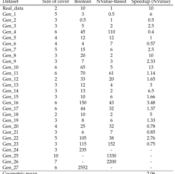
Table6.2shows a comparison between the processor time (in seconds) required by the Boolean and the NValue-based models. Both models were implemented in Sicstus Prolog and (in gen-eral terms) NValue proved to be much more efficient than the Boolean one, with a geometric average speedup of 2.06. This is due to the fact that the search space of this model only contains feasible solutions, and there are very efficient filtering algorithms of the NValue constraint.
6.3
The NValue constraint
In order to understand the subtleties behind this model, the NValue global constraint will be now analyzed in detail. This constraint was also partially implemented in CaSPER to try to find particular variations of it that may be useful in optimizing it to this particular use. CaSPER is a C++ library for generic constraint solving.
The NValue constraint is a generalization of both AtleastNValue and AtMostNValue, that will be presented later. It constraints the vectorX¯ of variables so that it uses exactlyNdifferent values. It prunes both the finite domain variableN and the vectorX¯. It must be noticed that sinceNis a finite domain variable, this constraint can be used to state upper and lower bounds for the cardinality ofX¯. This is achieved by propagating the following constraint:
AtMostNValue(X¯,N)∧AtLeastNValue(X¯,N)
6. ANEW MINIMIZINGNVALUE-BASED MODEL 6.3. The NValue constraint
Dataset Size of cover Boolean NValue-Based Speedup (NValue)
Real_data 2 10 1 10
Gen_1 5 3 0.5 6
Gen_2 3 0.5 1 0.5
Gen_3 3 5 2 2.5
Gen_4 6 45 110 0.4
Gen_5 4 12 12 1
Gen_6 4 4 7 0.57
Gen_7 5 15 6 2.5
Gen_8 3 20 2 10
Gen_9 3 7 3 2.33
Gen_10 6 65 5 13
Gen_11 6 70 61 1.14
Gen_12 2 33 20 1.65
Gen_13 3 12 4 3
Gen_14 3 13 2 6.5
Gen_15 3 10 6 1.66
Gen_16 6 150 43 3.48
Gen_17 6 44 32 1.37
Gen_18 2 10 2 5
Gen_19 3 8 6 1.33
Gen_20 4 25 32 0.78
Gen_21 3 6 7 0.85
Gen_22 5 105 38 2.76
Gen_23 3 115 152 0.75
Gen_24 3 235 -
-Gen_25 10 - 1330
-Gen_26 7 - 2200
-Gen_27 6 2552 -
-Geometric mean 2.06
6. ANEW MINIMIZINGNVALUE-BASED MODEL 6.4. The AtMostNValue constraint
those are necessarilymin(N) andmax(N), so it is enough to prohibit any valuebetweenmin(N) andmax(N).
Putting it all together, the filtering algorithm for the NValue constraint is schematized as:
NValue(X¯,N)≡
AtLeastNValue(X¯,N)∧AtMostNValue(X¯,N)
|D(N)|=2∧min(N) +1<max(N) =⇒
AtLeastNValue(X¯,max(N))
∨
AtMostNValue(X¯,min(N))
6.4
The AtMostNValue constraint
Given a vector of variablesX¯ and a finite domain variable N, the AtMostNValue constraint states that at mostN different values will be used byX¯. This constraint does not only filter the domains of the variables inX¯ but also the minimum value ofN. There are many filtering algorithms for this constraint and three have been analyzed in [BHH+06]. The algorithm that proved to be the most efficient in practice makes use of the concept of theindependence number
of a graph related to the vectorX¯. This number is directly linked to the lower bound of the cardinality of X¯, referred to as card↓(X¯). Although obtaining this number is an intractable problem, an approximation of it is used to prune the domain ofNand of the variables inX¯.
6.4.1 Graph theoretic concepts
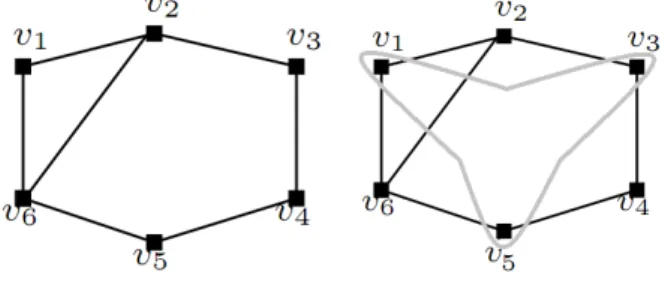
Given a family of sets F ={S1, ...,Sn} and a graph G= (V,E) with the set of vertices V =
{v1, ...,vn}and a set of edgesE,Gis theintersection graphofF iff
∀i,j<vi,vj>∈E ⇐⇒ Si∩Sj6=/0
that is to say that the intersection graph ofF is a graph that has arcs between each pair of sets inF that share elements. Given a vector of variablesX¯, the intersection graph of it is denoted byGX¯ = (V,E)whereV={v1, ...,vn}and∀i,j<vi,vj>∈E ⇐⇒ D(Xi)∩D(Xj)6=/0.
Theneighborhoodof a nodevis the set of nodes in the graph that are connected tovthrough edges. Thedegreeof a nodevis the size of its neighborhood.