EdilEan KlEbErda Silva bEjarano aragón MarcElo Savino Portugal
Resumo
Neste trabalho, examinamos se os efeitos das ações de política monetária sobre o produto são assimétricos no Brasil. Para isto, estimamos modelos Markov-switching que permitem que choques positivos e negati-vos afetem a taxa de crescimento do produto de forma assimétrica nos estados de expansão e recessão econômica. Em geral, os resultados mostram que: i) os efeitos reais de choques monetários negativos são maiores do que os de choques positivos em uma expansão; ii) em uma recessão, os efeitos reais de choques positivos e negativos são iguais; iii) não há evidência de assimetria entre os efeitos de políticas monetárias contracíclicas; iv) não se pode afirmar que os efeitos de choques positivos (ou negativos) dependem da fase do ciclo econômico.
PalavRas-chave
política monetária, assimetrias, choques negativos e positivos, ciclo de negócios, modelos Markov-switching
AbstrAct
In this paper, we check whether the effects of monetary policy actions on output in Brazil are asymmetric. Therefore, we estimate Markov-switching models that allow positive and negative shocks to affect the growth rate of output in an asymmetric fashion in expansion and recession states. In general, results show that: i) the real effects of negative monetary shocks are larger than those of positive shocks in an expansion; ii) in a recession, the real effects of positive and negative shocks are the same; iii) there is no evidence of asymmetry between the effects of countercyclical monetary policies; and iv) it is not possible to assert that the effects of a positive (or negative) shock are dependent upon the phase of the business cycle.
Keywords
monetary policy, asymmetries, positive and negative shocks, business cycle, Markov-switching models
JEL clAssificAtion
E52, E32, C32
Professor of Economics at UFPB. Endereço para contato: Universidade Federal da Paraíba – CCSA – Departamento
de Economia – Cid. Universitária – João Pessoa – PB – Brasil. CEP: 58059-900. Fone: (83)3216-7482. Email: eks_ cme@yahoo.com.br
Professor of Economics at UFRGS and CNPq researcher. E-mail: msp@ufrgs.br.
1 IntRoductIon
In recent times, the literature on asymmetric real effects of monetary policy has focused essentially on two types of asymmetry: (1) asymmetry related to the direc-tion of the monetary policy acdirec-tion; and (b) asymmetry related to the phase of the business cycle in place at the time at which this policy was adopted.1 The asym-metry related to the direction of the monetary policy action is found in models that yield a convex aggregate supply curve due to a stronger nominal rigidity to reduce the price and/or wage levels.2 In these models, positive monetary shock leads to a higher frequency of price adjustments, while a negative monetary shock produces a major effect on the output level of firms.3 This implies that the real effects of a contractionary monetary policy are larger than those of an expansionary one. On the other hand, the asymmetry related to the phase of the business cycle may be observed in models with credit market frictions generated by asymmetric informa-tion between lenders and borrowers.4 Since the amount of collaterals is smaller in a recession, the financial stance of economic agents is weaker and the supply of credit by commercial banks is smaller than during an expansion, and the external finance premium is higher in this phase of the business cycle. As a result, monetary policy shocks may have greater effects on output during a recession.
Several works have provided empirical evidence of different types of asymmetry in the effects of monetary policy on output. For example, Lemgruber (1980) points out that the real effects of a contractionary monetary policy are larger than those of an expansionary policy in Brazil. For the United States, Cover (1992), De Long and Summers (1988), Rhee and Rich (1995) and Karras and Stokes (1999) also found that negative monetary shocks had larger real effects than did positive shocks. Garcia and Schaller (2002), Dolado and Maria-Dolores (2001, 2006), Peersman and Smets (2001) and Kaufmann (2002) assessed asymmetry in the business cycle phase and found evidence that monetary policy actions have stronger effects on output in a recession in the U.S., Austrian, German, Spanish, Italian, French, and Belgian economies.
1 There exists a third type of asymmetry, which is related to large and small monetary shocks (BALL; ROMeR, 1989). It was not within the scope of the present paper to look into this type of asymmetry.
2 The Keynesian model with downward nominal wage rigidity and the asymmetric adjustment cost mod-els analyzed by Caballero and engel (1993), Tsiddon (1993) and Ball and Mankiw (1994) are included in this class of models.
3 Positive monetary shocks can be defined as unanticipated increases in money supply or unanticipated decreases in the interest rate of the monetary policy. Conversely, negative monetary shocks are un-anticipated decreases in money supply or unun-anticipated increases in the interest rate of the monetary policy.
The major aim of the present work is to investigate whether the effects of mone-tary policy on output are asymmetric in Brazil. Specifically, we seek to answer the following questions: i) in a given state of the business cycle, are the real effects of a contractionary monetary policy different from the effects of an expansionary one? ii) do the real effects of a countercyclical monetary policy depend on the state of the business cycle in place at the time at which the policy was implemented? iii) are the real effects of a contractionary (or expansionary) policy different between the phases of the business cycle?
In order to achieve our goal, we first measured monetary policy shocks and then we built positive and negative monetary shock series. Thereafter, we assessed the different types of asymmetry by extending the Markov-switching model developed by Hamilton (1989). In particular, we considered a specification of the Markov-switching model that allows positive and negative shocks to asymmetrically affect the rate of GDP growth during expansions and recessions. To check whether the real effects of monetary shocks are asymmetric, we performed a set of Wald tests and imposed different restrictions on the estimated parameters.
An important aspect of the analysis of monetary policy effects is the choice of the monetary policy instrument and consequently of the measure of policy actions. We chose the Selic rate as policy instrument because we believe this variable properly shows the main monetary policy actions taken by the Central Bank in the post-Real Plan period. After that, we measured monetary policy actions based on the innova-tions of a vector autoregressive model in which the Selic rate is included as one of the system variables. To check the robustness of results, we estimated the Markov-switching model using structural monetary shocks obtained from the estimation of different VAR model specifications and the Selic rate variation as a monetary policy instrument.
Two were our contributions to the existing empirical literature. First, we assessed the asymmetry related to the direction of the shock and also the asymmetry during expansions and recessions. Several macroeconomists tend to conflate these two types of asymmetry, thinking that monetary policy actions are typically countercyclical, in such a way that an analysis of the asymmetry between an expansionary and contractionary policy allows inferring on the asymmetry between expansions and recessions. However, Kaminsky et al. (2004) provide a body of evidence suggesting that monetary policy is procyclical in emerging economies (e.g.: Brazil).
(2005), Céspedes et al. (2005) and Fernandes and Toro (2005) have provided empi-rical evidence that monetary policy actions affect the real side of the Brazilian eco-nomy. Nevertheless, none of these studies considered that such effects were likely to be asymmetric in terms of economic conditions and/or nature of the policy action.
Besides the introduction, this paper is organized into four sections. Section 2 ou-tlines the empirical model and the statistical tests we are going to use to assess the different types of asymmetry in the real effects of the monetary policy. Section 3 describes the time series used. Section 4 presents and analyzes the results. Section 5 concludes.
2 EMPIRIcal MEtHodology
2.1 Econometric Model
To check whether the real effects of monetary policy are asymmetric, we extend Hamilton’s (1989) model, which allows positive and negative monetary shocks to asymmetrically affect the output growth rate between expansions and recessions. This model has the following advantages: i) the selection of states is jointly deter-mined with the estimation of the model parameters; ii) a greater relative weight is placed upon the observations that correspond more clearly to this state when esti-mating the coefficients of a given state; iii) the model allows jointly assessing the different types of asymmetric effects of monetary policy on output.
A more general specification of the Markov-switching model is given by:
1
1 1
1 1
,1 1 , ,1 1 ,
(
)
...
(
)
...
...
t t t p
t t p t t p
t s t s p t p s
S t S p t p S t S p t p t
y
y
y
u
u
u
u
− −
− − − −
− −
− − − − + + + +
− − − −
D − µ = φ D
− µ
+ + φ D
− µ
+
γ
+ + γ
+ γ
+ + γ
+ ε
2
~ . . .
(0,
)
t
i i d N
ε
σ
0
(1
)
1t
s
s
ts
tµ = µ
−
+ µ
(1)1,1 0,1
(1
1)
1,1 1t
S−
s
ts
t− − −
− −
γ
= γ
−
+ γ
,1 0,1
(1
1)
1,1 1t i
S−
s
ts
t+ + +
− −
where Δyt is the growth rate of the real Brazilian GDP,
t
s
µ
is the mean state-depen-dent growth rate of output,u
t i−
− is a negative monetary shock, St i−,i
−
γ
is thestate-dependent coefficient measuring the response of Δyt to a negative monetary shock,
i
u
+ is a positive monetary shock and St i−,i+
γ
is the state-dependent coefficientmeasu-ring the response of Δyt to a positive monetary shock. The state variable St suppose-dly assumes value 0 when the economy is in a recession and value 1 when it is in an expansion. Thus, the model parameters in a recession are
µ
0, 0,i−
γ
and 0,i+
γ
, whereas, in an expansion, these parameters are given byµ
1, 1,i−
γ
and 1,i+
γ
. The generating process of regimes st involves a first-order Markov-switching process and two states, whose supposedly ergodic and irreducible transition probability matrix is given by:1
1
p
q
P
p
q
−
=
−
(2)where
1
Pr[
t0 |
t0]
p
=
S
=
S
−=
1
1
− =
p
Pr[
S
t=
1|
S
t−=
0]
1
Pr[
t1|
t1]
q
=
S
=
S
−=
1
1
− =
q
Pr[
S
t=
0 |
S
t−=
1]
(3)
We assume transition probabilities to be constant in time and determined by the following logistic functions:
0 1
0
exp(
)
Pr[
0 |
0]
1 exp(
)
t t
p
=
S
=
S
−= =
θ
+
θ
(4)1 1
1
exp( )
Pr[
1|
1]
1 exp( )
t t
q
=
S
=
S
−= =
θ
+
θ
(5)where θ0 and θ1 are unrestricted parameters. Based on the probabilities in (4) and (5), one can calculate the mean duration (dst) of economic recession and expansion regimes by using expressions 1/(1-p) and 1/(1-q), respectively. The duration of each regime can be different, but it will be constant in time since the transition prob-ability matrix is fixed.5
2.1.1 determination of the number of Regimes
For the specification of the Markov-switching model, it is important to know wheth-er it provides a more adequate charactwheth-erization of data comparatively to a model with constant coefficients. A formal procedure is to use the likelihood ratio (LR) statistic to test the null hypothesis that a one-regime process generates data that run counter to the alternative hypothesis that these data are generated by a two-regime model. However, this test is problematic because regularity conditions are not maintained under the null hypothesis due to the presence of nuisance parameters and singularity of the information matrix (HANSeN, 1992). An alternative to the formal test of hypothesis is to choose the number of Markov states based on information criteria, such as Akaike (AIC), Schwarz (SC), Hannan-Quinn (HQ) and Markov-switching criterion (MSC).6
In this paper, we use three procedures to check whether the Markov-switching mo-del is more appropriate than the linear momo-del. The first two use the AIC and MSC, expressed by:
^
2 (
L
y
t, )
2
N
AIC
T
T
−
D λ
=
+
(6)^ ^
1 ^
^ 0
(
2 )
2 (
, )
2
2
l l t
l l
T T
K
MSC
L
y
T
K
=
+
= −
D λ +
−
−
∑
(7)where
^
( t, )
L D λy is the value of the log-likelihood function in ^
λ = λ
, n is the numberof parameters of the model, t is the number of observations, T0 =
∑
tPr(St =0 |IT),1 tPr( t 1| T)
T =
∑
S = I , Pr(st=st |IT) is the smoothed probability of regime st (0,1) and K is the number of explanatory variables plus the constant term. The third procedure consists of the approximation to the asymptotic distribution of the LR statistics proposed by Ang and Bekaert (1998). As shown by these authors, the asymptotic distribution of the LR statistic between 1 and 2 regimes can be approximated by a chi-square distribution, where the number of degrees of freedom is given by the number of nuisance parameters of the two-regime model plus the number of linear restrictions imposed on the one-regime model by the two-regime model.2.2 symmetry tests for the Real Effects of Monetary shocks
After estimating model (1), we tested the possible asymmetries in the real effects of the monetary policy by imposing restrictions on the sum of parameters t,
j S i
γ
, where j=-,+ and i=1,...,p. In particular, we test the following null hypotheses of symmetry:symmetry in the effects of positive and negative monetary shocks
0 0, 0,
1 1
:
p p
i i
i i
H − = +
= γ = γ
∑ ∑
(8)0 1, 1,
1 1
:
p p
i i
i i
H − = +
= γ = γ
∑ ∑
(9)symmetry in the effects of countercyclical monetary shocks
0 0, 1,
1 1
:
p p
i i
i i
H + = −
= γ = γ
∑ ∑
.(10)
symmetry in the effects of monetary shocks between recessions and expansions
0 0, 1,
1 1
:
p p
i i
i i
H − = −
= γ = γ
∑ ∑
(11)0 0, 1,
1 1
:
p p
i i
i i
H + = +
= γ = γ
∑ ∑
(12)The statistical significance of the restrictions imposed on the model is assessed by the usual Wald test. Under null hypotheses (8) through (12), the Wald test has a chi-square distribution with 1 degree of freedom.
3 data
as ln(yt/yt-1)x100, where ln denotes the natural logarithm. The series of the seasonally adjusted industrial production index was obtained from IBGe.7
The series of monetary shocks (ut) is obtained through the estimation of a vector autoregressive (VAR) model of order p. We estimate the VAR model using three variables: i) the natural logarithm of the industrial production index; ii) the monthly inflation rate defined by ln(IPCAt/ IPCAt-1)x100, where IPCA is the Brazilian con-sumer price index calculated by IBGe; iii) monthly overnight interest rate (SeLIC), regarded as a monetary policy instrument. The data used were obtained from the Central Bank of Brazil and from IBGe. The VAR is estimated using monthly data for the period between January 1995 and August 2006. We followed the recom-mendation of Sims (1980) and Doan (1992) and included all the variables in levels in the VAR model.8
The selection of order p was based on the multivariate AIC, SC and HQ criteria and also on the results of multivariate LM tests for autocorrelation of the system residuals, White test for the heteroskedasticity of system residuals and of each equa-tion, LM-ARCH test for autoregressive conditional heteroskedasticity (ARCH) in the residuals of each equation and the Jarque-Bera (JB) test for normality of residu-als. Given that the VAR(1) through VAR(4) models present autocorrelation and/ or heteroskedasticity problems, we decided to use VAR(5) in order to obtain the monetary shock series (ut).
The residuals of the Selic rate equation do not necessarily represent a true monetary shock, since they can be correlated with the residuals of other equations in the VAR model. Thus, to estimate structural monetary shocks, we followed the recursive identification framework proposed by Sims (1980) – Choleski’s orthogonalization. The ordering of variables in the VAR model was output, inflation, and Selic rate. Since monthly data are used, it is reasonable to assume that the output and infla-tion rate are not contemporaneously affected by the Selic rate. The imposiinfla-tion that the monetary policy reacts contemporaneously to output shocks and to shocks to the inflation rate is quite arguable since the data on inflation and output are made publicly available with some delay. Nevertheless, it is plausible to assume that by deciding on the value of the Selic rate in a given month the Central Bank has access to some current indicators of aggregate output and inflation.
7 IBGe – Brazilian Institute of Geography and Statistics.
After obtaining the structural monetary shock series (u), the next step involved obtaining different types of the shocks taken into consideration in model (1). We followed Cover (1992) and obtained the series of positive and negative monetary shocks using the following definitions:
min( , 0)
max( , 0)
t t
t t
u
u
u
u
+
−
=
=
(13)where
u
t+ is a positive monetary shock and
t
u
− is a negative monetary shock.To check the robustness of results, we did two exercises. The first one was obtaining
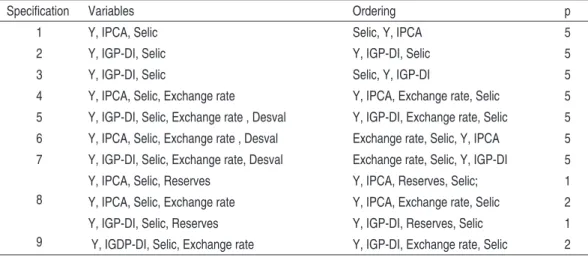
ut from the estimation of VAR models with different variables and from the ordering of variables in the system. Table 2 shows the characteristics of the estimated specifi-cations. In the first specification, we assume that the Selic rate reacts with delay to shocks on output and inflation and that monetary shocks contemporaneously affect output and prices. In specifications 2 and 3, we measured inflation using the IGP-DI (General Price Index – Internal Supply). In order to capture the effects of external restrictions on monetary policy decisions, specifications 4 through 7 include the natural logarithm of the nominal exchange rate (average buying price) and a dummy variable (Desval) that assumes value 1 in the floating exchange rate period (1999:1-2006:8). Finally, we estimated VAR models for subsamples 1995:1-1998:12 and 1999:1-2006:8. external restrictions were captured by the inclusion of the natural logarithm of international reserves (concept of liquidity) in the first subsample and of the exchange rate in the second subsample.
taBlE 1 – EstIM atEd sPEcIfIcatIons of tHE vaR ModEl
Speciication Variables Ordering p 1 Y, IPCA, Selic Selic, Y, IPCA 5 2 Y, IGP-DI, Selic Y, IGP-DI, Selic 5 3 Y, IGP-DI, Selic Selic, Y, IGP-DI 5
4 Y, IPCA, Selic, Exchange rate Y, IPCA, Exchange rate, Selic 5 5 Y, IGP-DI, Selic, Exchange rate , Desval Y, IGP-DI, Exchange rate, Selic 5 6 Y, IPCA, Selic, Exchange rate , Desval Exchange rate, Selic, Y, IPCA 5 7 Y, IGP-DI, Selic, Exchange rate, Desval Exchange rate, Selic, Y, IGP-DI 5
8
Y, IPCA, Selic, Reserves Y, IPCA, Reserves, Selic; 1 Y, IPCA, Selic, Exchange rate Y, IPCA, Exchange rate, Selic 2
9
In the second exercise, we used the variation in the Selic rate as an alternative me-thod to measure monetary policy. This variable is not appropriate for measuring mo-netary policy shocks since it is partially endogenous. However, its use is acceptable given that the monetary shocks detected in the VAR model are generated regressors in (1). As pointed out by Pagan (1984), the presence of generated regressors may imply inconsistent standard deviations of the estimated parameters, as well as of the tests based on these standard deviations. Therefore, the use of a monetary policy instrument that is not a generated regressor is an important way to test the robust-ness of results. Since we considered the variation in the Selic rate a monetary policy measure, the negative “monetary shock” series (positive variations in the interest rate) and the positive ones (negative variations in the interest rate) were obtained according to the definitions described in (13).
4 REsults
In this section, we report the results of the Markov-switching models estimated to check whether the effects of the monetary policy on output are asymmetric. All estimates were made using the Optimum procedure of the Gauss software. The nu-merical optimization was made using the BFGS (Broyden, Fletcher, Goldfarb and Shanno) algorithm described in Gill et al. (1981).
A common difficulty in estimating Markov-switching models lies in the fact that the log-likelihood function does not have a global maximum (HAMILTON, 1991). Additionally, there are often several local maxima that yield similar values for the log-likelihood function, but different parameter estimates. Owing to these proble-ms, we used different initial values and we chose the model with the largest log-likelihood function value. When we estimated the Markov-switching specification using variations in the Selic rate as monetary policy measure, we noted that the local maximum with the largest log-likelihood function value was characterized by a tran-sition probability p close to zero and by filtered probabilities of recession (regime 0) that captured only outliers in the data. Since the models with these characteristics imply that only one state practically persists throughout the sample period, we con-sider an alternative local maximum whose estimate of the parameter vector allows assessing the periods of recession and expansion more properly.
4.1 Estimates for the Ms Model with vaR shocks
MS(2)-ARX1(p).9 We use a set of LR tests to determine the autoregressive order of the model. The results indicate that the optimal number of lags is p=7.
To check whether the selection of the MS(2)-ARX1(7) model is appropriate, we used two strategies. First, we used the AIC and MSC criteria and the LR test proposed by Ang and Bekaert (1998) in order to verify whether the Markov-switching model is more suitable than the model with constant coefficients. Second, we performed Ljung-Box (LB) and ARCH tests to check the absence of serial correlation and au-toregressive conditional heteroskedasticity in the standardized prediction errors in the MS(2)-ARX1(7) model. The MSC and the LR tests carried out for a significance level of 2% suggest that the two-regime model represents the data more appropriate-ly than the linear model. The specification test results suggest absence of significant autocorrelation and of ARCH effects in the prediction errors of the model.
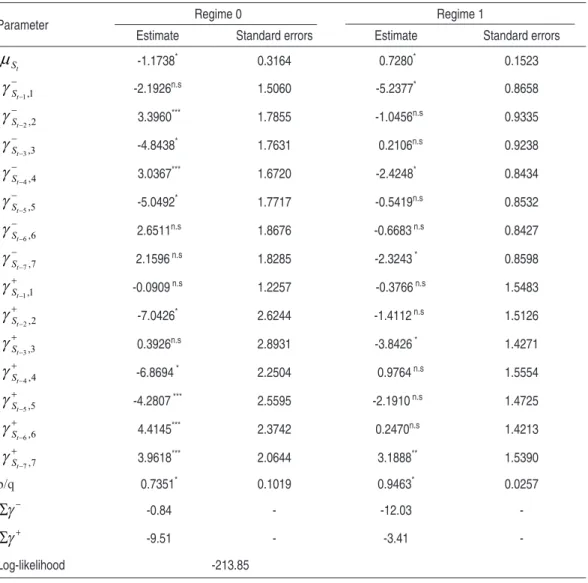
Table 2 shows the maximum likelihood estimates for the parameters of the MS(2)-ARX1(7) model.10 The estimated values for μ
St indicate that the economy has a mean growth rate of -1.17% per month (-14.04% per annum) in recessions (state 0) and of 0.728% per month (8.74% per annum) in expansions (state 1). The prob-abilities of remaining in each regime are estimated at 0.735 for state 0 and at 0.946 for state 1. This implies that recessions last on average 3.8 months, whereas periods of expansion last on average 18.64 months. All of these results indicate that the estimated Markov-switching model captures asymmetries in the business cycles, characterizing recessions as short periods of sudden drops in output and expansions as periods of gradual and lasting increase in output.
9 MS(2)-ARX1(p) denotes a two-regime Markov-switching model and p lags of the endogenous variable and of the exogenous regressors (positive and negative monetary shocks) obtained from a VAR. 10 In order to reduce the table size, we omitted the estimates for coefficients β’s and σ. Results can be
taBlE 2 – PaR aMEtER EstIMatIon foR tHE Ms(2)-aRX1(7) ModEl
Parameter Regime 0 Regime 1
Estimate Standard errors Estimate Standard errors
t
S
µ -1.1738* 0.3164 0.7280* 0.1523
1,1
t
S− −
γ -2.1926n.s 1.5060 -5.2377* 0.8658
2,2
t
S− −
γ 3.3960*** 1.7855 -1.0456n.s 0.9335
3,3
t
S− −
γ -4.8438* 1.7631 0.2106n.s 0.9238
4,4
t
S− −
γ 3.0367*** 1.6720 -2.4248* 0.8434
5,5
t
S− −
γ -5.0492* 1.7717 -0.5419n.s 0.8532
6,6
t
S− −
γ 2.6511n.s 1.8676 -0.6683 n.s 0.8427
7,7
t
S− −
γ 2.1596 n.s 1.8285 -2.3243 * 0.8598
1,1
t
S− +
γ -0.0909 n.s 1.2257 -0.3766 n.s 1.5483
2,2
t
S− +
γ -7.0426* 2.6244 -1.4112 n.s 1.5126
3,3
t
S− +
γ 0.3926n.s 2.8931 -3.8426 * 1.4271
4,4
t
S− +
γ -6.8694 * 2.2504 0.9764 n.s 1.5554
5,5
t
S− +
γ -4.2807 *** 2.5595 -2.1910 n.s 1.4725
6,6
t
S− +
γ 4.4145*** 2.3742 0.2470n.s 1.4213
7,7
t
S− +
γ 3.9618*** 2.0644 3.1888** 1.5390
p/q 0.7351* 0.1019 0.9463* 0.0257 −
Σγ -0.84 - -12.03
-+
Σγ -9.51 - -3.41
-Log-likelihood -213.85
Note: * Significant at 1%. ** Significant at 5%. *** Significant at 10%. n.s Not significant.
The behavior of the growth rate of output and of the probabilities of recession is shown in Figure 1. The filtered probability of recession can be understood as an optimal inference on this regime at time t using the information available up to time t, whereas the smoothed probability of recession is concerned with the infer-ence on this state using all the available information.11 By looking at Figure 1, one can perceive that the time paths of the filtered and smoothed probabilities are quite similar, suggesting that the estimates of recession periods can be obtained through recursive one-step ahead estimates (filtered probabilities) or by using all the available
information (smoothed probabilities). The specific dating of recession periods can be obtained by the rule that connects observation t to state 0 if the smoothed prob-ability of this regime is greater than 0.5 (HAMILTON, 1989). The application of this rule to the estimated model allows making a distinction between two periods of longer recessions (1998:7-1998:12 and 2001:3-2001:11) and two recessions with a duration no longer than three months (1997:4-1997:5 and 2002:12-2003:2). These results seem to be consistent with those obtained by Céspedes et al. (2006). 12
fIguRE 1 – BEHavIoR of tHE gdP gRowtH R atE and of fIltEREd and sMootHEd PRoBaBIlItIEs of R EcEssIon foR tHE Ms(2)-aRX1(7) ModEl
The effects of monetary shocks on output are measured by the sum of coefficients of each type of shock for each regime ( 0,
j i i
Σ γ and 1,
j i i
Σ γ , for j =-,+). The results shown in Table 2 suggest that an unexpected increase in the Selic rate lowers the output in both states of the business cycle, whereas an unexpected decrease in the Selic rate increases the aggregate output. Moreover, output appears to be more sensitive to negative monetary shocks during an expansion and less sensitive to them in a recession.
To determine the statistical significance of the effects of different monetary shocks, we performed a set of Wald tests and imposed different restrictions on the estimated parameters. The results of these tests are shown on the first eight lines of Table 3. On the first four lines, we test the null hypothesis that the coefficients related to a given monetary shock in a given regime are jointly equal to zero. In all cases, this null hypothesis is rejected at a 1% significance level. The subsequent four lines test whether the sum of the coefficients of each shock is equal to zero. Given a signi-ficance level of 10%, we can observe that this hypothesis is rejected only for the negative shocks in the state of expansion and positive shocks in the state of recession. This indicates that the effects of the procyclical monetary shocks on the output are neutral.
taBlE 3 – wald tEsts foR tHE Ms(2)-aRX1(7) ModEl
Null hypothesis Value of χ2 statistic No. of restrictions P-value
,
0,i 0 i
−
γ = ∀ 20.92 7 0.0039
, 1,i 0 i
−
γ = ∀ 52.42 7 0.0000
,
0,i 0 i
+
γ = ∀ 23.44 7 0.0014
, 1,i 0 i
+
γ = ∀ 19.42 7 0.0070
0,i 0
−
Σγ = 0.08 1 0.7773
1,i 0
−
Σγ = 22.04 1 0.0000
0,i 0
+
Σγ = 2.80 1 0.0943
1,i 0
+
Σγ = 0.98 1 0.3221
0,i 0,i
− +
Σγ = Σγ 2.17 1 0.1407
1,i 1,i
− +
Σγ = Σγ 3.60 1 0.0578
0,i 1,i
+ −
Σγ = Σγ 0.17 1 0.6801
0,i 1,i
− −
Σγ = Σγ 8.26 1 0.0041
0,i 1,i
+ +
Σγ = Σγ 1.19 1 0.2753
Now we check whether the effects of different monetary policy actions are asym-metric. To do that, we test the null hypotheses of symmetry explained in section 2.2. In Table 3, we highlight several results. First, the null hypothesis of symmetry between the effects of positive and negative shocks is not rejected at a 10% signifi-cance level in state 0, but it is rejected (in favor of 1,i 12.03 1,i 3.41
− +
6% significance level in state 1. This suggests that the real effects of negative mon-etary shocks are larger than the effects of positive shocks only in the expansion phase of the business cycle. Secondly, the non-rejection of the null hypothesis 0,i 1,i
+ −
Σγ = Σγ
shows that the impact on the output of a given unexpected decrease in the Selic rate in a recession is equivalent to that of an increase during an expansion. This indicates that the real effects of a countercyclical monetary policy do not depend on the pre-vailing state of the business cycle when monetary shock occurs. Thirdly, the Wald test result strongly rejects the null hypothesis that the real effects of negative shocks are the same between the Markov states in favor of a larger effect of these shocks in the expansion state ( 1,i 12.84 0,i 0.86
− −
Σγ = − > Σγ = − ). Finally, we cannot reject the null hypothesis of symmetry of real effects of positive monetary shocks between the states of the business cycle.
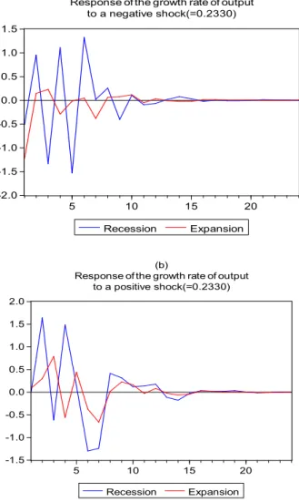
The differences in the real effects of the monetary policy are shown in Figure 2. In Panel a, we show the paths of the growth rate of output in a recession and in an expansion in response to a negative shock (or to an unexpected increase in the Selic rate) equal to 0.233 percentage points implemented at t=0.13 In Panel b, the responses of the growth rate of output to a positive shock of -0.233 percentage points are presented for the two Markov regimes. Initially, we can perceive that the oscillation in output in response to different types of monetary shocks is a com-mon characteristic in both panels. This probably results from the high noise level in the monthly series of the industrial production growth rate. When we compare the paths of output across the different regimes, we also note that the response of output has a greater variability in the recession phase of the business cycle for any of the types of shocks considered.
13 The value 0.2330 is the estimate for the standard deviation of the structural monetary shock series ut
fIguRE 2 – statE-dEPEndEnt EffEcts of a MonEtaRy sHocK In tHE vaR ModEl
-2.0 -1.5 -1.0 -0.5 0.0 0.5 1.0 1.5
5 10 15 20
Recession Expansion (a)
Response of the growth rate of output to a negative shock(=0.2330)
-1.5 -1.0 -0.5 0.0 0.5 1.0 1.5 2.0
5 10 15 20
Recession Expansion (b)
Response of the growth rate of output to a positive shock(=0.2330)
rea-ches its maximum in the second and third months during recession and expansion, respectively.
Finally, one can observe that the response of the growth rate of output accumulated in the 24 months after a negative (positive) shock is equal to -0.09% (1.02%) in the recession regime and to -1.3% (0.37%) in the expansion regime. The differences in these values suggest that: i) in the expansion regime, the negative shocks affect output more strongly than do positive shocks; ii) the real effect of a negative shock is larger during an expansion than in a recession; iii) in the recession regime, the real effect of a given positive shock outperforms, in absolute value, the effect of a negative shock; iv) the real effect of a positive shock is larger during an expansion; and v) the real effect of an unexpected increase in the Selic rate is larger than that of an unexpected decrease in this rate during recession. It is important that results iii through v be taken with caution, since the Wald tests did not reject the null hy-potheses of symmetry for these cases.
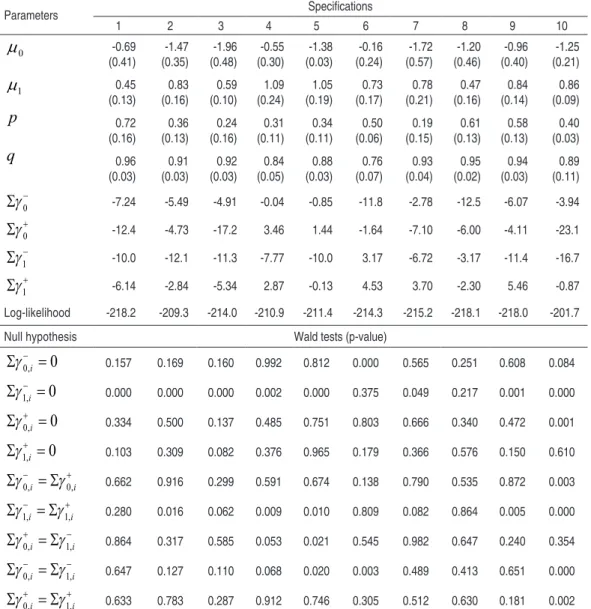
4.2 checking the Robustness of Results
taBlE 4 – M aRKov-swItcHIng ModEl EstIM atIon REsults
Parameters Speciications
1 2 3 4 5 6 7 8 9 10
0
µ -0.69
(0.41) (0.35)-1.47 (0.48)-1.96 (0.30)-0.55 (0.03)-1.38 (0.24)-0.16 (0.57)-1.72 (0.46)-1.20 (0.40)-0.96 (0.21)-1.25
1
µ 0.45
(0.13) (0.16) 0.83 (0.10) 0.59 (0.24) 1.09 (0.19) 1.05 (0.17) 0.73 (0.21) 0.78 (0.16) 0.47 (0.14) 0.84 (0.09) 0.86
p 0.72 (0.16) 0.36 (0.13) 0.24 (0.16) 0.31 (0.11) 0.34 (0.11) 0.50 (0.06) 0.19 (0.15) 0.61 (0.13) 0.58 (0.13) 0.40 (0.03) q 0.96
(0.03) (0.03) 0.91 (0.03) 0.92 (0.05) 0.84 (0.03) 0.88 (0.07) 0.76 (0.04) 0.93 (0.02) 0.95 (0.03) 0.94 (0.11) 0.89
0
−
Σγ -7.24 -5.49 -4.91 -0.04 -0.85 -11.8 -2.78 -12.5 -6.07 -3.94
0
+
Σγ -12.4 -4.73 -17.2 3.46 1.44 -1.64 -7.10 -6.00 -4.11 -23.1
1
−
Σγ -10.0 -12.1 -11.3 -7.77 -10.0 3.17 -6.72 -3.17 -11.4 -16.7
1
+
Σγ -6.14 -2.84 -5.34 2.87 -0.13 4.53 3.70 -2.30 5.46 -0.87
Log-likelihood -218.2 -209.3 -214.0 -210.9 -211.4 -214.3 -215.2 -218.1 -218.0 -201.7
Null hypothesis Wald tests (p-value)
0,i 0
−
Σγ = 0.157 0.169 0.160 0.992 0.812 0.000 0.565 0.251 0.608 0.084
1,i 0
−
Σγ = 0.000 0.000 0.000 0.002 0.000 0.375 0.049 0.217 0.001 0.000
0,i 0
+
Σγ = 0.334 0.500 0.137 0.485 0.751 0.803 0.666 0.340 0.472 0.001
1,i 0
+
Σγ = 0.103 0.309 0.082 0.376 0.965 0.179 0.366 0.576 0.150 0.610
0,i 0,i
− +
Σγ = Σγ 0.662 0.916 0.299 0.591 0.674 0.138 0.790 0.535 0.872 0.003
1,i 1,i
− +
Σγ = Σγ 0.280 0.016 0.062 0.009 0.010 0.809 0.082 0.864 0.005 0.000
0,i 1,i
+ −
Σγ = Σγ 0.864 0.317 0.585 0.053 0.021 0.545 0.982 0.647 0.240 0.354
0,i 1,i
− −
Σγ = Σγ 0.647 0.127 0.110 0.068 0.020 0.003 0.489 0.413 0.651 0.000
0,i 1,i
+ +
Σγ = Σγ 0.633 0.783 0.287 0.912 0.746 0.305 0.512 0.630 0.181 0.002
fIguRE 3 – BEHavIoR of tHE gdP gRowtH R atE and sMootHEd PRoBaBIlItIEs of REcEssIon foR tHE Ms ModEls
1 -6 -4 -2 0 2 4 6 -2 -1 0 1 2
96 97 98 99 00 01 02 03 04 05 06
Rate of GDP growth Smoothed probability
2 -6 -4 -2 0 2 4 6 -2 -1 0 1 2
96 97 98 99 00 01 02 03 04 05 06
Rate of GDP growth Smoothed probability
3 -6 -4 -2 0 2 4 6 -2 -1 0 1 2
96 97 98 99 00 01 02 03 04 05 06
Rate of GDP growth Smoothed probability
4 -6 -4 -2 0 2 4 6 -2 -1 0 1 2
96 97 98 99 00 01 02 03 04 05 06
Rate of GDP growth Smoothed probability
5 -6 -4 -2 0 2 4 6 -2 -1 0 1 2
96 97 98 99 00 01 02 03 04 05 06
Rate of GDP growth Smoothed probability
6 -6 -4 -2 0 2 4 6 -2 -1 0 1 2
96 97 98 99 00 01 02 03 04 05 06
Rate of GDP growth Smoothed probability
7 -6 -4 -2 0 2 4 6 -2 -1 0 1 2
96 97 98 99 00 01 02 03 04 05 06
Rate of GDP growth Smoothed probability
8 -6 -4 -2 0 2 4 6 -2 -1 0 1 2
96 97 98 99 00 01 02 03 04 05 06
Rate of GDP growth Smoothed probability
9 -6 -4 -2 0 2 4 6 -2 -1 0 1 2
96 97 98 99 00 01 02 03 04 05 06
Rate of GDP growth Smoothed probability
10 -6 -4 -2 0 2 4 6 -2 -1 0 1 2
96 97 98 99 00 01 02 03 04 05 06
In regard to the real effects of structural monetary shocks, Table 4 shows that, in general, the estimates of the sum of coefficients associated with each type of shock have the expected sign. For specifications in which the effects of monetary shocks differ from those theoretically predicted, the Wald tests do not reject the null hypo-thesis that these effects are statistically equal to zero. Furthermore, note that null hypotheses H0: γ0,i 0
−
Σ = and H0: γ1,i 0
+
Σ = are not rejected in most of the estimated specifications. This corroborates the result obtained in the previous section, indica-ting the neutrality of the real effects of procyclical monetary shocks. As to coun-tercyclical monetary shocks, the Wald tests show that, in general, we can reject the null hypothesis of neutrality of negative shocks, but this is not true for positive shocks. The result of the neutrality of positive monetary shocks differs from that one obtained by the model in the previous section and this is observed in all Markov-switching specifications using structural monetary shocks.
When the Selic rate is used to measure monetary policy actions, we can observe that the sum of the coefficients related to each “shock” suggests that a positive variation in the Selic rate reduces output, whereas a negative variation increases output. The Wald test results support the non-neutrality of the effects of positive variations in the Selic rate in both states of the business cycle. As far as negative variations in the Selic rate are concerned, we found evidence that the sum of the coefficients related to this policy action is statistically different from zero only in the recession state.
5 conclusIons
In this paper, we sought to empirically investigate whether the real effects of mone-tary policy in Brazil are asymmetric in terms of the direction of the monemone-tary policy action and of the phase of the business cycle in place at the time at which the policy was implemented. The empirical strategy we used consisted of a two-step estimation procedure. First, we measured monetary policy actions based on the innovations of a vector autoregressive model in which output, inflation rate and Selic rate are included as system variables. After that, we estimated an extended specification of the Markov-switching model proposed by Hamilton (1989), which allows positive and negative monetary shocks to asymmetrically affect the growth rate of output during expansions and recessions. To check the robustness of results, we estimated the Markov-switching model using structural monetary shocks obtained from the estimation of different VAR model specifications and the Selic rate variation as a monetary policy instrument.
We assessed whether the effects of the monetary policy on output are asymmetric by using the Wald statistics to test a set of null hypotheses of symmetry in the effects of different shocks. For most of the estimated specifications, we found evidence of asymmetry between the real effects of contractionary and expansionary monetary policies in the expansion regime. This result is consistent with the existence of a convex aggregate supply curve resulting from downward price and wage rigidity. With regard to the recession state, there was no evidence of asymmetry between the effects of positive and negative monetary shocks. A possible explanation is that recession periods were frequently adjusted for months of sudden and transient de-creases in output (e.g., 1998:09-10, 2001:09-10 and 2002:12-2003:1), which proves a major obstacle to the assessment and differentiation of the real effects of positive and negative monetary shocks in this Markov state.
the effects of a contractionary monetary policy implemented during an expansion and those of an expansionary policy implemented during a recession.
REfEREncEs
ANG, A.; BeKAeRT, G. Regime switches in interest rates. Cambridge: National Bureau of economic Research, 1998. (Working Paper, 6508).
BALL, L.; ROMeR, D. Are prices too sticky?the Quarterly Journal of Economics, v. 104, n.3, 1989.
BALL, L.; MANKIW, N. G. Asymmetric price adjustment and economic fluctua-tions. the Economic Journal, v. 104, n. 423, 1994.
BeRNANKe, B.; GeRTLeR, M. Agency cost, net worth, collateral, and business fluctuations. american Economics Review, v. 79, n. 1, 1989.
______. Inside the black box: the credit channel of monetary policy transmission. the Journal of Economic Perspectives, v. 9, n. 4, 1995.
BeRNANKe, B.; MIHOV, I. What does the Bundesbank target? European Economic Review, v. 41, n. 6, 1997.
______. Measuring monetary policy. the Quarterly Journal of Economics, v. 113, n.3, 1998.
CABALLeRO, R. J.; eNGeL, e.M.R.A. Heterogeneity and output fluctuations in a dynamic menu-cost economy. Review of Economic studies, v. 60, n. 202, 1993. CÉSPeDeS, B. J. V.Monetary policy, inflation and the level of economic activity in Brazil
after the real plan: stylized facts from svaR models.Rio de Janeiro: IPeA, 2005.
(Discussion Paper, 1101).
______ et al.Forecasting Brazilian output and its turning points in the presence of breaks: a comparison of linear and nonlinear models. Estudos Econômicos, v. 36, n. 1, 2006.
COVeR, J. P. Asymmetric effects of positive and negative money-supply shocks. the
Quarterly Journal of Economics, v.107, n. 4, 1992.
De LONG, J. B.; SUMMeRS, L. H. How does macroeconomic policy affect output?
Brookings Papers on Economic activity, v. 1988, n. 2, 1988.
DOAN, T. Rats user’s manual. evanston: estima, 1992.
DOLADO, J.J.; MARIA-DOLOReS, R. An empirical study of the cyclical effects of monetary policy in Spain.Investigaciones Económicas, v. 25, n. 1, 2001. ______. State asymmetries in the effects of monetary policy shocks on output: some
DRIFFILL, J.; SOLA, M. Intrinsic bubbles and regime-switching. Journal of Monetary Economics, v. 42, n. 2, 1998.
FeRNANDeS, M.; TORO, J. Mecanismo de transmissão monetária na economia brasileira pós-plano Real. Revista Brasileira de Economia, v.59, n. 1, 2005. GARCIA, R.; SCHALLeR, H. Are the effects of monetary policy asymmetric?
Economic Inquiry, v. 40, n. 1, 2002.
GeRTLeR, M.; HUBBARD, R. G. financial factors in business fluctuations.
Cambridge: National Bureau of economic Research, 1988. (Working Paper, 2758).
GILL, P. e. et al. Practical optimization. London: Academic Press, 1981.
GOODWIN, T. H. Business-cycle analysis with a Markov-switching model. Journal of Business and Economic statistics, v. 11, n. 3, 1993.
HAMILTON, J. A new approach to the economic analysis of nonstationary time series and the business cycle. Econometrica, v. 57, n. 2, 1989.
______. A quasi-Bayesian approach to estimating parameters for mixtures of normal distributions. Journal of Business and Economic statistics, v. 9, n.1,1991.
______. time series analysis. Princeton: Princeton University Press, 1994.
HANSeN, B. e. The likelihood ratio test under nonstandard conditions: testing the Markov switching model of GNP. Journal of applied Econometrics, v. 7, 1992. HeNDRY, D. F. dynamic econometrics. Oxford: Oxford University Press, 1996. KAMINSKY, G. L. et al. when it rains, it pours: procyclical capital flows and
macr-oeconomic policies. Cambridge: National Bureau of economic Research, 2004.
(Working Paper, 10780).
KARRAS, G.; STOKeS, H. H. Why are the effects of money-supply shocks asymmetric? evidence from prices, consumption, and investment. Journal of
Macroeconomics, v. 21, n. 4, 1999.
KAUFMANN, S. Is there an asymmetric effect of monetary policy over time? A Bayesian analysis using Austrian data. Empirical Economics, v. 27, n.2, 2002. KIM, C-J. Dynamic linear models with Markov-switching. Journal of Econometrics,
v. 60, n. 1-2, 1994.
______ et al. Is there a positive relationship between stock market volatility and the equity premium? Journal of Money, credit, and Banking, v. 36, n. 3, 2004. LeMGRUBeR, A. C. expectativas racionais e o dilema produto real/inflação no
Brasil. Revista Brasileira de Economia, v. 34, n. 4, 1980.
MAHeU, J. M.; McCURDY, T. H. Identifying bull and bear markets in stock returns. Journal of Business and Economics statistics, v. 18, n. 1, 2000.
MOReIRA, A. et al. os impactos das políticas monetária e cambial no Brasil pós-Plano
Real. Rio de Janeiro: IPeA, 1998. (Texto para Discussão, 579).
PAGAN, A. econometric issues in the analysis of regressions with generated regressors.
International Economic Review, v. 25, n. 1, 1984.
PeeRSMAN, G.; SMeTS, F. are the effects of monetary policy in the Euro area greater
in recessions than in booms? Frankfurt: european Central Bank, 2001. (Working
Paper, 52).
PSARADAKIS, Z; SPAGNOLO, N. On the determination of the number of regimes in Markov switching autoregressive models. Journal of time series analysis, v. 24, n. 2, 2003.
RABANAL, P., SCHWARTZ, G. Testing the effectiveness of the overnight interest rate as a monetary policy instrument. Brazil: selected issues and statistical appen-dix. Washington D.C.: International Monetary Fund, 2001. (Country Report, 01/10).
RAVN; M. O.; SOLA, M. Asymmetric effects of monetary policy in the United States.Review of federal Reserve Bank of st. louis, v. 86, n. 5, 2004.
RHee, W.; RICH, R. W. Inflation and asymmetric effects of money on output fluctuations. Journal of Macroeconomics, v. 17, n. 4, 1995.
SIMS, C. Macroeconomics and reality. Econometrica, v. 48, n. 1, 1980.
______ et al.Inference in linear time-series models with some unit roots. Econometrica, v. 58, n. 1, p. 113-144, 1990.
SMITH, A. et al. Markov-switching model selection using Kullback–Leibler diver-gence. Journal of Econometrics, v. 134, n. 2, 2006.