Rev. Bras. Econ. vol.57 número3

(1)

Andr´e Minella**

Summary: 1. Introduction; 2. Methodology; 3. Results; 4. Con-clusions.

Keywords: monetary policy; inﬂation; interest rate; money; Brazil. JEL codes: E31; E52.

This paper investigates monetary policy and basic macroeconomic relationships involving output, inflation rate, interest rate, and money in Brazil. Based on a vector autoregressive (VAR) esti-mation, it compares three different periods: moderately-increasing inflation (1975–1985), high inflation (1985–1994), and low inflation (1994–2000). The main results are the following: monetary policy shocks have significant effects on output; monetary policy shocks do not induce a reduction in the inflation rate in the first two peri-ods, but there are indications that they have gained power to affect prices after the Real Plan was launched; monetary policy does not usually respond rapidly or actively to inflation-rate and output in-novations; in the recent period, the interest rate responds intensely to financial crises; positive interest-rate shocks are accompanied by a decline in money in all the three periods; the degree of inflation persistence is substantially lower in the recent period.

Este artigo examina a pol´ıtica monetária e rela¸cões macroeconô-micas básicas envolvendo produto, infla¸cão, taxa de juros e moeda no Brasil. Baseando-se em uma estimativa de um vetor auto-regressivo (VAR), comparam-se três per´ıodos: infla¸cão moderada-mente crescente (1975–1985), alta infla¸cão (1985–1994) e baixa infla¸cão (1994–2000). Os principais resultados são os seguintes: choques na pol´ıtica monetária têm efeitos significativos no produto; choques na pol´ıtica monetária não induzem uma redu¸cão na taxa de infla¸cão nos dois primeiros per´ıodos, mas há indica¸cões de que eles

*

This paper was received in Dec. 2001 and approved in Aug. 2002. I am grateful to Mark Gertler, Ali Hakan Kara, Kenneth Kuttner and two anonymous referees for their helpful com-ments and suggestions. All remaining errors are my responsibility. Financial support from the Central Bank of Brazil and CAPES is gratefully acknowledged. The views expressed are those of the author and not necessarily those of the Central Bank of Brazil or its members. E-mail: andre.minella@bcb.gov.br.

**

Research Department, Central Bank of Brazil.

(2)

aumentaram seu poder de afetar pre¸cos depois que o Plano Real foi implementado; a pol´ıtica monetária geralmente não responde ativa ou rapidamente frente a choques na taxa de infla¸cão e no produto; no per´ıodo recente, a taxa de juros responde intensamente a crises financeiras; choques positivos na taxa de juros são acompanhados por um decl´ınio na quantidade de moeda em todos os três per´ıodos; o grau de persistência inflacionária é significativamente menor no per´ıodo recente.

1. Introduction

This paper investigates monetary policy and basic macroeconomic relation-ships involving output, inflation rate, interest rate, and money in Brazil. Based on a vector autoregressive (VAR) estimation, the paper addresses the following ques-tions: do monetary policy shocks have real effects?; do monetary policy shocks affect inflation rate?; what is the reaction of monetary policy to inflation-rate, output, and financial shocks?; is inflation rate persistent?; what is the relation between money and interest rate?

Furthermore, the objective is to compare these relationships across different periods. Because of the limited availability of data, the sample estimation goes from 1975 to 2000. The inflation rate, measured as percentage variation per month, and its first difference are presented in figure 1. Based on the behavior of the inflation rate and stabilization policies, the macroeconomic context in Brazil can be divided into three periods:

• Moderately-increasing inflation (1975–1985). Inflation rate was increasing, but at a slower rate than the prevailing in the following nine years. There was no stabilization program that produced an abrupt reduction in the inflation rate;

• High inflation (1985–1994). Inflation rate grew at a fast rate. There were five stabilization programs, usually involving price freeze without previous announcement. Their success were just momentary: the inflation rate fell abruptly, but sooner or later it increased again;

(3)

Figure 1

Selected Variables: 1975-2000 (Monthly Data)

Industrial Production Index (Y) - Log Level

log level

1975 1978 1981 1984 1987 1990 1993 1996 1999 420

440 460 480 500

First Difference of Y

%

1975 1978 1981 1984 1987 1990 1993 1996 1999 -30 -20 -10 0 10 20 30

Inflation Rate - IGP-DI (INF)

% per month

1975 1978 1981 1984 1987 1990 1993 1996 1999 -12 0 12 24 36 48 60 72 84

First Difference of INF

% per month

1975 1978 1981 1984 1987 1990 1993 1996 1999 -75

-50 -25 0 25

Nominal Interest Rate (INT)

% per month

1975 1978 1981 1984 1987 1990 1993 1996 1999 0 10 20 30 40 50 60 70 80 90

First Difference of INT

% per month

1975 1978 1981 1984 1987 1990 1993 1996 1999 -50 -40 -30 -20 -10 0 10 20

Growth Rate of M1 (GRM1)

% per month

1975 1978 1981 1984 1987 1990 1993 1996 1999 -25 0 25 50 75 100 125

First Difference of GRM1

% per month

1975 1978 1981 1984 1987 1990 1993 1996 1999 -100 -80 -60 -40 -20 0 20 40 60

In particular, the change from a high to a low-inflation environment is expected to be accompanied by an increase in the effectiveness of monetary policy. One reason is the reduction in the degree of inflation persistence in the recent period, which is verified by the estimation in this paper.1

For the OECD countries, the literature that investigates monetary policy and macroeconomic relationships using a VAR estimation is vast.2 For Brazil, in con-trast, only more recently the VAR approach has been employed. For the periods

1

Other factors that would increase the effectiveness of monetary policy are stressed by Lopes (1997): a lower inflation-rate volatility premium, an expected longer maturity of assets that would raise the wealth effect of an increase in the interest rate, the expansion in credit that has accompanied the stabilization, and the adoption of a floating exchange-rate regime expanding the exchange-rate channel.

2

(4)

before the recent stabilization program, Pastore (1995, 1997) has found passiveness of money supply to the inflation rate, and high degree of inflation persistence.3 In terms of comparison across periods, Fiorencio and Moreira (1999) have concluded that, during 1982–1994, monetary policy did not practically affect unemployment and price level, whereas, for 1994–1998, positive interest-rate shocks increased unemployment and decreased price level. For 1995–2000, Rabanal and Schwartz (2001) have found a negative response of output and money to interest-rate shocks. Nevertheless, I consider that it is necessary an investigation that covers a large span, addresses all the questions previously mentioned, and compares results across the three different periods.

In spite of the instability of the Brazilian economy, several important results emerge from the estimations in this paper. First, monetary policy shocks have important real effects on the economy. Positive shocks to the interest rate lead to a decline in output in all the three periods analyzed. The effect seems to be more pronounced after the Real Plan was launched. Second, despite the real effects, monetary policy shocks do not generate a reduction in the inflation rate during the first two periods. For the Real Plan period, however, there is some evidence that monetary policy has gained power to curb inflation, although the results are not conclusive. Third, regarding the reaction of monetary policy, the interest rate does not respond actively or at least rapidly to inflation-rate innovations: the re-sponse of the nominal interest rate, in the first two months, is smaller than the rise in the inflation rate in all the three periods analyzed. Similarly, the interest rate does not react to stabilize output. In the Real Plan period, monetary policy responds strongly to financial crises. Fourth, the degree of inflation persistence has clearly decreased in the recent period. Fifth, a positive interest-rate innova-tion is accompanied by a decline in money in all the periods. In fact, there is some evidence of a negative correlation between money supply and interest rate. Furthermore, inflation-rate innovations induce a decline in the real money levels. The results are also consistent with the fact that the Central Bank targets the interest rate instead of M1.

Section 2 deals with the methodology used for the estimation, and section 3 presents the results. A ﬁnal section concludes the paper.

2. Methodology

The paper considers the following dynamic model:

3

(5)

AoZt = k+ p

i=1

AiZt−i+ut (1)

where:

Zt is the (n x 1) vector of variables;

Ao and Ai are (n x n) matrices of coeﬃcients; k is a vector of constants;

p is the number of lags, and

ut is a vector of uncorrelated white noise disturbances (E(utu′

t) is assumed to be a diagonal matrix). Premultiplying byA−1

o , we obtain the reduced form for the VAR:

Zt = c+ p

i=1

BiZt−i+εt (2)

where: c =A−1

o k;

Bi = A−o1Ai (for i= 1,2, ..., p), and

εt =A−o1ut is white noise with variance-covariance matrix Φ =A−o1E(utu

′

t) (A−1

o )

′

.4

The estimated VAR (equation 2) includes basically four variables: output (Y), measured by the index of industrial production produced by IBGE (seasonally adjusted); inflation rate (INF) or price level (P) measured by IGP-DI;5 nomi-nal interest rate (INT), given by the Selic overnight interest rate (interest rate in overnight operations between banks involving government debt as collateral – analogous to the fed funds rate); and the monetary aggregate M1. The estimation uses monthly data.6 Figure 1 shows these variables and their first differences for 1975-2000.

4

Hamilton (1994).

5

IGP-DI is produced by FGV, and is a weighted average of indexes of wholesale prices, consumer prices, and construction costs.

6

The values for the interest rate and monetary aggregate employed are the average during the month. For M1, between 1975:01 and 1979:12, we have only data corresponding to the balance at the end of month. In this case, I have estimated the value for month t using the arithmetic average of the balances between the end of months t−1 andt. The data source for the interest

(6)

The questions are investigated using orthogonalized impulse-response func-tions, which describe the response of a variable to a one-time shock to one of the elements of ut. This paper uses a Cholesky decomposition to identify the or-thogonalized disturbances ut. This recursive structure means, for example, that,

contemporaneously, the first variable in the ordering is not affected by shocks to the other variables, but shocks to the first variable affect the other ones; the second variable affects the third and fourth ones, but it is not affected contem-poraneously by them, and so on. I have assumed the following ordering: output, inflation rate, nominal interest rate, and M1 (“benchmark ordering”). Decisions of production level tend to respond with some delay. Thus, using monthly data, it seems reasonable to assume that output does not respond contemporaneously to other shocks. The inflation rate is assumed to respond contemporaneously to output innovations, but not to interest-rate and M1 shocks. Since the interest rate is adjusted basically on a daily basis, it can react very quickly to output and inflation-rate shocks. Because of the presence of delays in the availability of out-put and inflation-rate data, I have assumed that there are some current indicators for these variables. Finally, shocks to output, inflation rate and interest rate are assumed to be transmitted rapidly to the monetary aggregate.

Because of the important differences in the dynamics of the inflation rate and the other two nominal variables across the three mentioned periods, the paper esti-mates separate VARs for each period. The subsamples are the following: 1975:01 – 1985:07 (first subsample), 1985:08 – 1994:06 (second subsample), 1994:09 – 2000:12 (third subsample). The vertical lines in figure 1 divide the periods accordingly.

The series of the inflation rate and other nominal variables present important breaks immediately after the launch of six stabilization programs. The estimation for the second subsample includes two impulse dummies for each program (except for the first program, for which was used one dummy). These dummies assume the value of one for the selected month, and zero otherwise.7 Because of the fast acceleration of the inflation rate before the Collor Plan, launched in March 1990, I have added a dummy variable that takes the value of one in the three months previous to that plan. The estimation also includes centered seasonal dummies for all variables. Thus, the estimated model corresponds to equation (2), but with the addition of all these dummy variables.

As a result of the breaks, usual critical values for the cointegration tests can-not be used. Johansen et al. (2000) have addressed the cointegration test in the presence of breaks. Nevertheless, since there is a great number of breaks in the

7

(7)

Brazilian series (at least ﬁve in the second subsample), and most of them are rel-atively close to each other, I have estimated the model using I(1) – integrated of order one – regressors instead of employing the error correction representa-tion. The estimation is consistent and captures possible existing cointegration relationships (Sims et al., 1990, Watson, 1994). The main drawbacks are that usual Granger causality tests are not valid, and tests for structural breaks are also aﬀected.

It is a highly difficult task to determine the order of integration of the variables because the breaks affect the unit root tests. Cati et al. (1999) have constructed a test for series with this kind of break with an application to the inflation rate in Brazil for 1974:01 to 1993:06. They have found mixed results, but have concluded that we cannot reject the unit root hypothesis. They have also mentioned that found similar results for the nominal interest rate.

I have followed Cati, Garcia, and Perron’s results. For the second subsample, which presents several breaks, I have treated the inﬂation rate and nominal interest rate as I(1). Since the dynamics of the nominal variables are dominated by the inﬂation rate, I have also assumed that the growth rate of M1, denoted by GRM1, is I(1).

I have conducted unit root tests for output for all subperiods, and for the nominal variables for the first and third periods, which present no break. I have used the Augmented Dickey-Fuller test, where the null hypothesis is that the variable is I(1). The lag length was chosen using the Akaike Information Criterion (AIC). The results are shown in table A.1 in the Appendix. For the output, we reject the null of presence of a unit root for the whole sample (1975:01 – 2000:12) and second subsample, and we accept it for the first and third subsamples. I have treated output as I(1) in all estimations. For the nominal interest rate, we can accept the null of unit root for the first and third subsamples. I have also used the multiple unit root test, procedure based on Dickey and Pantula (1987) to deal with cases where a higher than one order of differencing is necessary. In this case, the null hypothesis is that the variable is I(2). In the first period, using the multiple unit root test, we can accept that the price log-level is I(2). Therefore, we can accept that the inflation rate is I(1). For the third subsample, the results are clear: using the Augmented Dickey-Fuller test, we reject the null of I(1) for the inflation rate and accept it for the price log-level, and, using the multiple unit root test, we reject the null of I(2) for the price log-level.8 As a consequence,

8

(8)

the main specification for the third subsample uses price log-level as variable. In order to compare results, I have also estimated using the inflation rate. The tests for the growth rate of M1 in the first period are not conclusive. Nonetheless, it seems reasonable to consider the M1 growth rate and the inflation rate as having the same order of integration, possibly being cointegrated.9 Thus, I have treated the growth rate of M1 as I(1). For the third subsample, we can accept the null that the M1 log-level is I(1), and, using the multiple unit root test, we reject the null hypothesis that M1 log-level is I(2). Consequently, I have used M1 log-level as variable in the third subsample, besides estimating using M1 growth rate to compare results.

Therefore, most of the estimations are conducted using as variables: log-level of the index of industrial production, inflation rate, level of nominal interest rate, and M1 growth rate (“growth-rate specification”). The third subsample is also estimated employing the “level specification”: price and M1 log-levels instead of the inflation rate and M1 growth rate.10

The lag length for the VAR estimation was selected using AIC, but the residuals were also tested for autocorrelation and autoregressive conditional heteroskedas-ticity (ARCH). Sometimes, it was necessary to add one or two lags to obtain better residuals.11

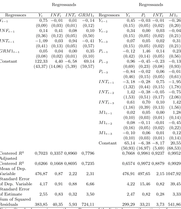
Table 1 presents the residual analysis of the benchmark estimations and the respective selected lag lengths.12 Autocorrelation – LM(1) and LM(4) refer to the lagrange multiplier test for the ﬁrst and fourth order autocorrelation of the residuals, respectively. The null hypothesis is that the residuals do not present serial correlation of ﬁrst or fourth order. ARCH refers to a lagrange multiplier test for autoregressive conditional heteroskedasticity of order equal to the number of lags in the model. The null hypothesis is absence of autoregressive conditional heteroskedasticity. The following line refers to a test where the null hypothesis is

inﬂation rate to its own shock.

9

Pastore (1994/1995) has found that money growth and inﬂation rate are cointegrated for 1944 – 1985.

10

I show the results using the inﬂation rate and the growth rate of M1 estimated directly as (xt₋xt₋1)/xt₋1, wherextis the price or the M1 level. Qualitatively, the results are very similar

to those using log-diﬀerences. In the case of the level speciﬁcation for the third subsample, I have used log(1 +i) for the nominal interest rate, where iis the interest rate in fractional units.

11

I have also estimated all the three subsamples using four lags – the maximum lag length used across the subsamples – to verify if the results are dependent on the diﬀerence of lag length. The main results remain unchanged.

12

(9)

normality of residuals. All the values shown are p-values. In general, the results are poor in terms of normality, but satisfactory for autocorrelation and conditional heteroskedasticity.13 The estimates of the regressions are presented in table A.2 in the Appendix.

Table 1

Test for autocorrelation, ARCH, and normality of residuals (p-values)

First Subsample (3 lags)

Test System Y INF INT GRM1

Autocorrelation - LM(1) 0.42 0.07 0.35 0.63 0.46 Autocorrelation - LM(4) 0.13 0.19 0.07 0.28 0.60

ARCH 0.15 0.34 0.16 0.90

Normality 0.00 0.52 0.00 0.04 0.00

Second Subsample (4 lags)

ARCH 0.98 0.81 0.59 0.56

Normality 0.00 0.03 0.00 0.00 0.00

Third Subsample - growth-rate speciﬁcation (1 lag)

ARCH 0.21 0.53 0.86 0.35

Normality 0.00 0.00 0.00 0.00 0.00

Third Subsample - level speciﬁcation (3 lags)

ARCH 0.92 0.89 0.95 0.84

Normality 0.00 0.00 0.00 0.00 0.00

Notes: The null hypothesis are the following: absence of serial corre-lation of ﬁrst and fourth orders (Autocorrecorre-lation - LM(1) and (4)); absence of autoregressive conditional heteroskedasticity (ARCH), and normal distribution of residuals.

13

(10)

The impulse-response functions and their two-standard-error bands were esti-mated using a Monte Carlo experiment based on Doan (2000, p. 398). The values are expressed as percentage (output, price level, M1 level) or percentage points (inﬂation rate, interest rate, M1 growth rate) deviations from a no-shock case, all measured as percentage per month. The value of the shock is one standard deviation of the residual of the variable unless explicitly noted otherwise.

I have conducted several exercises of robustness. For the second and third subsamples, I have also estimated using a different price index, IPCA (available since 1980), which is a consumer price index produced by IBGE that has been recently used in the inflation targeting regime (adopted since July 1999). For the second subsample, the results are qualitatively the same as those with IGP-DI, whereas for the third subsample there are some differences, which are discussed along the text. When the index used is not mentioned, the estimation employs IGP-DI.

In addition, since in the recent period the interest-rate responded to the fi-nancial external crises (Mexico, Asia, Russia) and to the exchange-rate crisis in Brasil at the beginning of 1999, I have also estimated, for the third subsample, a five-variable model that includes the spread of the Emerging Markets Bond In-dex (EMBI) relative to U.S. treasuries (estimated by J. P. Morgan). The EMBI spread is considered a good indicator for these crises because it increased signifi-cantly during these episodes. The estimation uses the level of EMBI spread, which appears before the nominal interest rate and money in the ordering. We accept the null hypothesis of presence of a unit root for EMBI spread (table A.1).

(11)

rate, output, and M1 growth rate (or M1 level). In this case, the interest rate reacts contemporaneously to inﬂation-rate shocks, but not to output shocks. The conclusions of the paper do not change with these two orderings.14 A three-variable VAR that excluded money was estimated as well. The results (not related to money) are also unchanged.

The benchmark model does not include exchange rate among the variables. The reasons are the following. First, the paper does not involve the assessment of the exchange rate. Second, Brazil had several exchange rate regimes and maxide-valuations. The model estimation would have to take into consideration these changes, perhaps implying different identification structures across regimes. Third, if we include the exchange rate, it would be more interesting to add exports and imports to the model as well. In this case, however, the model becomes very large and should be used to address other questions (effect of devaluations on trade balance, etc.). Still, for robustness purposes, I have conducted some estimations including the exchange rate. One consequence is that residuals become less well behaved. In particular, I have compared the results for the Real Plan using a five-variable model with the ordering output, inflation rate (or price level), growth rate of nominal exchange rate (or exchange rate level), nominal interest rate, and the growth rate of M1 (or M1 level). The impulse-response functions using IPCA are very similar to those obtained with the four-variable model. In the case of IGP-DI, the main differences are noted in the respective sections.

3. Results

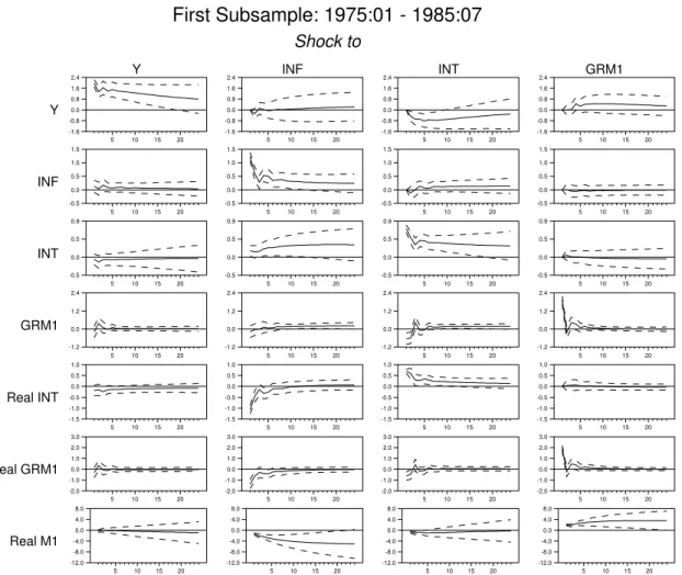
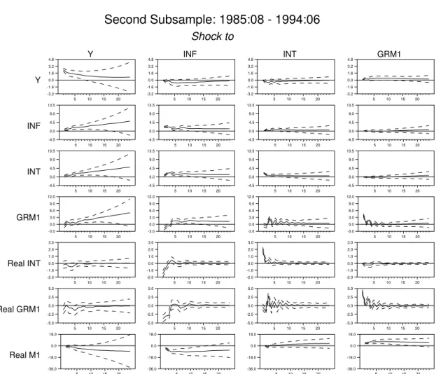
The impulse-response functions (solid lines) and their two-standard-error ban-ds (dashed lines) for the benchmark ordering with IGP-DI as the price index are shown in figures 2 to 5.15 Each column represents the responses of the different variables to a specific shock. Figures 2 to 4 refer to the three subsamples using the growth-rate specification. Figure 5 refers to the third subsample employing the level specification (price and M1 levels). Besides the path of the estimated variables, the figures also show some nominal variables in real terms, such as the real interest rate, real money growth, and real money level, which are estimated using the respective values of the current inflation rate. In each figure, the graphs in a given row have the same scale.

14

The results are not shown, but are available upon request. The main diﬀerence refers to the contemporaneous reaction of some variables because of the ordering used.

15

(12)

Figure 2

First Subsample: 1975:01 - 1985:07 Shock to Y INF INT GRM1 Real INT Real GRM1 Real M1

Y INF INT GRM1

5 10 15 20 -1.6 -0.8 0.0 0.8 1.6 2.4

5 10 15 20 -0.5

0.0 0.5 1.0 1.5

5 10 15 20 -0.5

0.0 0.5 0.9

5 10 15 20 -1.2

0.0 1.2 2.4

5 10 15 20 -1.5 -1.0 -0.5 0.0 0.5 1.0

5 10 15 20 -2.0 -1.0 0.0 1.0 2.0 3.0

5 10 15 20 -12.0 -8.0 -4.0 0.0 4.0 8.0

5 10 15 20 -1.6 -0.8 0.0 0.8 1.6 2.4

5 10 15 20 -0.5

0.0 0.5 1.0 1.5

5 10 15 20 -0.5

0.0 0.5 0.9

5 10 15 20 -1.2

0.0 1.2 2.4

5 10 15 20 -1.5 -1.0 -0.5 0.0 0.5 1.0

5 10 15 20 -2.0 -1.0 0.0 1.0 2.0 3.0

5 10 15 20 -12.0 -8.0 -4.0 0.0 4.0 8.0

5 10 15 20 -1.6 -0.8 0.0 0.8 1.6 2.4

5 10 15 20 -0.5

0.0 0.5 1.0 1.5

5 10 15 20 -0.5

0.0 0.5 0.9

5 10 15 20 -1.2

0.0 1.2 2.4

5 10 15 20 -1.5 -1.0 -0.5 0.0 0.5 1.0

5 10 15 20 -2.0 -1.0 0.0 1.0 2.0 3.0

5 10 15 20 -12.0 -8.0 -4.0 0.0 4.0 8.0

5 10 15 20 -1.6 -0.8 0.0 0.8 1.6 2.4

5 10 15 20 -0.5

0.0 0.5 1.0 1.5

5 10 15 20 -0.5

0.0 0.5 0.9

5 10 15 20 -1.2

0.0 1.2 2.4

5 10 15 20 -1.5 -1.0 -0.5 0.0 0.5 1.0

5 10 15 20 -2.0 -1.0 0.0 1.0 2.0 3.0

(13)

Figure 3

Second Subsample: 1985:08 - 1994:06 Shock to Y INF INT GRM1 Real INT Real GRM1 Real M1

Y INF INT GRM1

5 10 15 20 -3.2 -1.6 0.0 1.6 3.2 4.8

5 10 15 20 -4.5

0.0 4.5 9.0 13.5

5 10 15 20 -4.5

0.0 4.5 9.0 13.5

5 10 15 20 -3.0 0.0 3.0 6.0 9.0 12.0

5 10 15 20 -2.0 -1.0 0.0 1.0 2.0 3.0

5 10 15 20 -5.0

-2.5 0.0 2.5 5.0

5 10 15 20 -36.0

-18.0 0.0 18.0

5 10 15 20 -3.2 -1.6 0.0 1.6 3.2 4.8

5 10 15 20 -4.5

0.0 4.5 9.0 13.5

5 10 15 20 -4.5

0.0 4.5 9.0 13.5

5 10 15 20 -3.0 0.0 3.0 6.0 9.0 12.0

5 10 15 20 -2.0 -1.0 0.0 1.0 2.0 3.0

5 10 15 20 -5.0

-2.5 0.0 2.5 5.0

5 10 15 20 -36.0

-18.0 0.0 18.0

5 10 15 20 -3.2 -1.6 0.0 1.6 3.2 4.8

5 10 15 20 -4.5

0.0 4.5 9.0 13.5

5 10 15 20 -4.5

0.0 4.5 9.0 13.5

5 10 15 20 -3.0 0.0 3.0 6.0 9.0 12.0

5 10 15 20 -2.0 -1.0 0.0 1.0 2.0 3.0

5 10 15 20 -5.0

-2.5 0.0 2.5 5.0

5 10 15 20 -36.0

-18.0 0.0 18.0

5 10 15 20 -3.2 -1.6 0.0 1.6 3.2 4.8

5 10 15 20 -4.5

0.0 4.5 9.0 13.5

5 10 15 20 -4.5

0.0 4.5 9.0 13.5

5 10 15 20 -3.0 0.0 3.0 6.0 9.0 12.0

5 10 15 20 -2.0 -1.0 0.0 1.0 2.0 3.0

5 10 15 20 -5.0

-2.5 0.0 2.5 5.0

5 10 15 20 -36.0

(14)

Figure 4

Third Subsample: 1994:09 - 2000:12 - Growth-Rate Spec. Shock to Y INF INT GRM1 Real INT Real GRM1 Real M1

Y INF INT GRM1

5 10 15 20 -2.0 -1.0 0.0 1.0 2.0 3.0

5 10 15 20 -0.2 0.0 0.2 0.5 0.8 1.0

5 10 15 20 -0.2

0.0 0.2 0.3

5 10 15 20 -2.0

0.0 2.0 4.0

5 10 15 20 -0.9

-0.5 0.0 0.5

5 10 15 20 -2.0

0.0 2.0 4.0

5 10 15 20 -7.0

-3.5 0.0 3.5 7.0

5 10 15 20 -2.0 -1.0 0.0 1.0 2.0 3.0

5 10 15 20 -0.2 0.0 0.2 0.5 0.8 1.0

5 10 15 20 -0.2

0.0 0.2 0.3

5 10 15 20 -2.0

0.0 2.0 4.0

5 10 15 20 -0.9

-0.5 0.0 0.5

5 10 15 20 -2.0

0.0 2.0 4.0

5 10 15 20 -7.0

-3.5 0.0 3.5 7.0

5 10 15 20 -2.0 -1.0 0.0 1.0 2.0 3.0

5 10 15 20 -0.2 0.0 0.2 0.5 0.8 1.0

5 10 15 20 -0.2

0.0 0.2 0.3

5 10 15 20 -2.0

0.0 2.0 4.0

5 10 15 20 -0.9

-0.5 0.0 0.5

5 10 15 20 -2.0

0.0 2.0 4.0

5 10 15 20 -7.0

-3.5 0.0 3.5 7.0

5 10 15 20 -2.0 -1.0 0.0 1.0 2.0 3.0

5 10 15 20 -0.2 0.0 0.2 0.5 0.8 1.0

5 10 15 20 -0.2

0.0 0.2 0.3

5 10 15 20 -2.0

0.0 2.0 4.0

5 10 15 20 -0.9

-0.5 0.0 0.5

5 10 15 20 -2.0

0.0 2.0 4.0

5 10 15 20 -7.0

(15)

Figure 5

Third Subsample: 1994:09 - 2000:12 - Level Specification Shock to Y P INT M1 Inflation GRM1 Real Int Real GRM1 Real M1

Y P INT M1

5 10 15 20 -1.4

0.0 1.4 2.8

5 10 15 20 -2.5

0.0 2.5 5.0

5 10 15 20 -0.2 -0.1 0.0 0.1 0.2 0.3

5 10 15 20 -5.0 -2.5 0.0 2.5 5.0 7.5

5 10 15 20 -0.5

0.0 0.5 0.9

5 10 15 20 -1.6

0.0 1.6 3.2

5 10 15 20 -0.9

-0.5 0.0 0.5

5 10 15 20 -1.8

0.0 1.8 3.6

5 10 15 20 -6.0

-3.0 0.0 3.0 6.0

5 10 15 20 -1.4

0.0 1.4 2.8

5 10 15 20 -2.5

0.0 2.5 5.0

5 10 15 20 -0.2 -0.1 0.0 0.1 0.2 0.3

5 10 15 20 -5.0 -2.5 0.0 2.5 5.0 7.5

5 10 15 20 -0.5

0.0 0.5 0.9

5 10 15 20 -1.6

0.0 1.6 3.2

5 10 15 20 -0.9

-0.5 0.0 0.5

5 10 15 20 -1.8

0.0 1.8 3.6

5 10 15 20 -6.0

-3.0 0.0 3.0 6.0

5 10 15 20 -1.4

0.0 1.4 2.8

5 10 15 20 -2.5

0.0 2.5 5.0

5 10 15 20 -0.2 -0.1 0.0 0.1 0.2 0.3

5 10 15 20 -5.0 -2.5 0.0 2.5 5.0 7.5

5 10 15 20 -0.5

0.0 0.5 0.9

5 10 15 20 -1.6

0.0 1.6 3.2

5 10 15 20 -0.9

-0.5 0.0 0.5

5 10 15 20 -1.8

0.0 1.8 3.6

5 10 15 20 -6.0

-3.0 0.0 3.0 6.0

5 10 15 20 -1.4

0.0 1.4 2.8

5 10 15 20 -2.5

0.0 2.5 5.0

5 10 15 20 -0.2 -0.1 0.0 0.1 0.2 0.3

5 10 15 20 -5.0 -2.5 0.0 2.5 5.0 7.5

5 10 15 20 -0.5

0.0 0.5 0.9

5 10 15 20 -1.6

0.0 1.6 3.2

5 10 15 20 -0.9

-0.5 0.0 0.5

5 10 15 20 -1.8

0.0 1.8 3.6

5 10 15 20 -6.0

-3.0 0.0 3.0 6.0

3.1 Inflation persistence

(16)

54.2% in the second one, whereas it is only 1.4% in the third subsample using the growth-rate specification (and 4.2% with the level specification). Therefore, the recent stabilization has been accompanied by a significant reduction in the degree of inflation persistence. One of the causes is the substantial decline in the use of indexation in the economy.

If we consider only the coefficients on the lagged inflation terms, which give the direct effect of past inflation in the current inflation, the third subsample presents a lower effect of past inflation. The sum of the coefficients on the lagged inflation terms are 0.81, 0.69, and 0.41 for the first, second, and third subsamples, respectively (table A.2).16

3.2 Real effects of monetary policy shocks

Perhaps the most robust result across subsamples and different estimation specifications is that a positive shock to interest rate reduces output. The rise in the nominal interest rate is accompanied by an increase in the real interest rate. The response of output is fast and hump-shaped. In the second month (with the ordering assumed, output does not respond in the first month), output is negative, and the estimate is statistically significant. The maximum reduction is reached between three and seven months, depending on the estimation. Qualitatively, this result is in line with the findings in Freitas and Muinhos (2001) and Andrade and Divino (2000), based on an IS curve estimation.17 The response is faster than those estimated for the U.S. and other OECD economies, where the response is also hump-shaped, but the maximum reduction in the output usually occurs between one and two years.18 The speed of the response in the Brazilian case may be related to the predominance of short-term credit, where the average interest rate charged in the outstanding debts responds more rapidly to changes in the basic interest rate.

16

Considering the same lag length for the three periods (four lags), the sums are 0.73, 0.69, and 0.41.

17

Freitas and Muinhos (2001) have estimated an IS equation for 1992:4 – 1999:1 with quarterly data. Real interest rate with a lag of one quarter enters significantly in the output-gap (GDP) regression with a negative sign. Likewise, Andrade and Divino (2000) have estimated an IS equation, but with monthly data from 1994:08 to 1999:03. The coefficient on the six-month lag of the real interest rate is negative and statistically significant in the output-gap (estimated GDP) regression.

18

(17)

Figure 6

Responses of output to an interest-rate shock: comparison across subsamples

1st Subsample 2nd Subsample

3rd Subsample - Growth-Rate Specification 3rd Subsample - Level Specification

5 10 15 20

-3.5 -3.0 -2.5 -2.0 -1.5 -1.0 -0.5 0.0 0.5

(18)

instability of the high-inﬂation period, however, we should be cautious with this ﬁnding.

In quantitative terms, during the Real Plan period, a one-percentage-point shock to interest rate – measured monthly – leads to a maximum decrease in the output of about 2.7% – 3.2%. Expressing interest rate in percentage per year, a one-percentage-point shock generates a maximum output reduction of approxi-mately 0.25%.

3.3 Effects of monetary policy shocks on the price level and

infla-tion rate

In spite of the similarities in terms of real effects, the effects of an interest-rate shock on price and inflation rate differ across periods. In the first subsample, there is no statistically significant effect on the inflation rate. In fact, the point estimates show some increase in the inflation rate. In the second subsample, there is an “inflation-rate puzzle”: a positive interest-rate innovation is followed by a rise in the inflation rate.19

During the high-inflation period, the inflation rate was increasing at a fast rate. Because the price index compares the average of prices during the current month to the average over the past month, when inflation rate is rapidly increasing, the index tends to underestimate the current inflation rate. Hence, part of the interest-rate innovation may reflect a response to an increasing inflation rate that does not appear integrally in the current price index. In this period, part of the agents, including the Central Bank, tended to use also a “centered” inflation rate to estimate the real interest rate. The centered inflation rate is calculated comparing the geometric average of the price index between months t and t+ 1 to the average betweent andt−1. Since it compares the average at the end of month t to that at the end of month t−1, it captures the acceleration of the inflation rate during the current month. Figure 7 shows the impulse-response function of the centered inflation rate to an interest-rate shock for the high-inflation period.

19

(19)

The inﬂation-rate puzzle disappears.20

Figure 7

Second subsample: response of the centered inﬂation rate to an interest-rate shock

-1.5 -1.0 -0.5 0.0 0.5 1.0 1.5

Most importantly, we can conclude that, for the first and second subsamples, monetary policy shocks do not induce a reduction in the inflation rate.21 This is consistent with the idea that, in a context of high inflation, inflation rate tends to respond very poorly to monetary policy.

For the third subsample, the results with the benchmark model are not con-clusive. Using the level specification (figure 5), a positive interest-rate shock is followed by a temporary decrease in the price level and inflation rate (inflation rate here is calculated as the log-difference of the price level response).22 Never-theless, when using the growth-rate specification (figure 4), the inflation rate does not respond to the interest-rate shock.23

20

This result, however, has to be considered cautiously because the estimation has problems of consistency. The centered inﬂation rate at t−1 is correlated with shocks at t. Besides, for

the first subsample, using the centered inflation rate, the response of the inflation rate becomes significantly positive.

21

With the specification for the second subsample using the centered inflation rate, the point estimates indicate a reduction in the inflation rate, but it is at most close to be significant, and lasts only one or two months.

22

Nonetheless, reducing the number of lags employed from three to two (not shown), the eﬀect disappears.

23

(20)

Figure 8

Third subsample: responses to an interest-rate schock using estimation including EMBIS - diﬀerent speciﬁcations

INF

INT

P

GR. Spec. w. IGP GR. Spec. w. IPCA Lev. Spec. w. IGP Lev. Spec. w. IPCA

-0.3 -0.2 0.0 0.2 0.3

-3.0 -2.0 -1.0 0.0 1.0

Nonetheless, the model may be misspecified since the interest rate reacted strongly to the financial crises during the Real Plan period. Figure 8 shows the impulse-response functions of inflation rate, nominal interest rate and price level to an interest-rate shock using the five-variable model that includes the EMBI spread (EMBIS). Each column refers to a different model specification. The rise in the nominal interest rate is also accompanied by an increase in the real interest

(21)

rate (not shown). With the growth-rate specification, there is a temporary decline in the inflation rate.24 Most importantly, with the level specification, using either IGP-DI or IPCA, there is a highly persistent decline in the price level.

Hence, it seems that monetary policy has gained power to aﬀect prices in the recent period, although the results are not conclusive.

3.4 Reaction of monetary policy to shocks

The paper evaluates the reaction of monetary policy to inflation-rate, out-put and financial shocks by the conduct of the interest rate rather than by the behavior of some monetary aggregate. There exists a pattern that holds in all subsamples: the nominal interest rate reacts positively to inflation-rate shocks, but the response is initially smaller than the rise in the inflation rate. At least during the first two months, the real interest rate is negative. There are several possible explanations for this behavior, which are not necessarily incompatible. A first explanation is based on the policy regime. The Central Bank may have reacted passively to inflation-rate shocks. A second possible interpretation relies on the practice of some interest-rate smoothing by the Central Bank. In reaction to shocks, the interest rate is not adjusted immediately to the value considered as optimal.25 We can expect, however, that the interest rate reaches its desired level after some time. A third explanation is that the monetary authority does not observe contemporaneously the inflation-rate shock. Nevertheless, we would expect that, in the following period, the Central Bank would adjust the interest rate accordingly. A fourth interpretation could be that the Central Bank reacts to the expected rather than to the current inflation rate. Nonetheless, since there is a considerable degree of inflation persistence, mainly in the first and second subsamples, we can also expect a strong reaction to the current inflation rate.

Unfortunately, the VAR approach does not allow to determine specifically which one of these explanations is more appropriate. Nevertheless, in all the four mentioned cases, we can consider that the path of the interest rate, at least after the initial months, can be used as one of the indicators to assess whether the central bank reacts actively or passively to inflation-rate shocks. It is important to stress that the paper does not use the average real interest rate to assess monetary policy, but the reaction of the interest rate to innovations to the inflation rate and output.

24

Hence, the inﬂation-rate puzzle veriﬁed when using IPCA is eliminated.

25

(22)

After the two-month horizon, the interest-rate behavior presents some differ-ences across periods. In the first subsample, the real interest rate is still negative at least over the following three months, and is not significantly different from zero after that.

In the high-inflation period, the real interest rate is significantly positive in the fourth month, but returns to zero in the sixth month. The reaction of the monetary authority seems to be stronger than that in the first subsample. Since the significant positive real interest rate lasts only one month, we cannot regard this as an active reaction of monetary policy.26 On the other hand, given the small sensitivity of the inflation rate to monetary policy shocks in the moderately-increasing- and high-inflation periods, the incentives to a more active monetary policy are low.

For the third subsample, the results are mixed. Using the level specification, the impulse response refers to shocks to the price level. The real interest rate is basically zero as of the third month.27 In contrast, employing the growth-rate specification, the real interest growth-rate is positive and statistically significant over several months, but the result is not robust.28

We can conclude that, in general, the interest rate responds with some delays to inﬂation-rate shocks, and that the ﬁrst subsample shows a weaker response of the monetary authority.

Regarding the reaction to output innovations in the moderately-increasing-and high-inﬂation periods, it seems that the interest rate does not react to stabilize output (the response of the interest rate, measured in real terms, is negative or not positive). For the Real Plan period, the results are not conclusive.29

Nonetheless, the reaction of monetary policy to the financial crises is evident during the Real Plan period. Figure 9 presents the impulse-response functions of the EMBI spread and nominal interest rate according to different model specifi-cations. All specifications show a strong response of the interest rate to a shock to the EMBI spread.

26

Using IPCA, the reaction is a little stronger: the point estimates of the real interest rate are positive between the second and fourth months (signiﬁcant in the third month).

27

Including the exchange rate in the estimation, the response of the real interest rate to a price level shock is positive and signiﬁcant in the fourth month.

28

In the estimation, augmenting the number of lags from one to two, including the exchange rate, or using IPCA changes the results.

29

(23)

Figure 9

Third subsample: responses to an EMBIS shock - diﬀerent speciﬁcations

EMBIS

INT

GR. Spec. w. IGP GR. Spec. w. IPCA Lev. Spec. w. IGP Lev. Spec. w. IPCA

-1.5 -1.0 -0.5 0.0 0.5 1.0 1.5

-0.4 -0.2 0.0 0.2 0.4

3.5 Reaction of money to inflation-rate shocks

Most of the estimations show a zero or positive response of money to inﬂation. A positive response of money supply, however, does not necessarily represent a passive monetary policy. Indeed, nominal money supply can rise, even when the central bank conducts an active monetary policy, considered here as an increase in the nominal interest rate in a greater proportion than the rise in the inﬂation rate.30

30

(24)

In all subsamples, an inflation-rate shock generates a decline in the real money levels.31 The real money reduction extends approximately over the period in which the inflation-rate response is still positive. Since the response of the real interest rate is not usually positive, I do not conclude that the decrease in the real money levels reflects an active monetary policy. I interpret it as a consequence of the fall in the demand for real money balances resulting from the increase in the opportunity cost of holding money.

3.6 Interest rate and money

Liquidity eﬀect refers to a negative response of the interest rate to a rise in the money supply. Unfortunately, the model used does not allow to isolate the money supply shocks.32 Nevertheless, some results emerge regarding the relation between interest rate and money, the identiﬁcation of a monetary policy shock, and the conduct of monetary policy.

The subsection considers two issues. The ﬁrst is whether a positive interest-rate shock is accompanied by a decline in the level or growth interest-rate of money. The second is whether a positive money shock is accompanied by a decrease in the interest rate.

In general, the results indicate a negative response of money to interest-rate shocks, although temporary in some cases. These results are robust to the alter-native ordering of the variables, where money appears before interest rate.33 In terms of real balances, most of the subsamples show that an interest-rate shock leads to a fall in the real money level, although usually temporary. This result is also robust to the alternative ordering.34

cost of holding money, we would observe an expansion in the money supply. In fact, we could find that inflation rate Granger causes money supply. Similarly, an increase in the growth rate of money smaller than the rise in the inflation rate cannot necessarily be associated with an active monetary policy because it can be the result of the lower demand for real balances.

31

Except for the third subsample using IPCA.

32

Part of the controversy of the empirical veriﬁcation of the liquidity eﬀect is related to the inappropriate treatment of innovations to monetary aggregates as shocks to monetary policy. See Bernanke and Mihov (1998a).

33

There are some exceptions, however, in the third subsample. With the growth-rate specifica-tion using IGP-DI, there is no response of M1 growth rate. Employing IPCA, with the growth-rate formulation, the response is negative, although not significant, whereas with the level specifica-tion, there is no response. Figures with the impulse-response functions to interest-rate and money innovations using the alternative ordering are available upon request.

34

(25)

The finding of a negative response of money to a positive interest-rate shock is consistent with interpreting the interest-rate innovation as a monetary policy shock. Central banks, by operating in the open market, sell bonds to raise interest rate, reducing monetary reserves and thus affecting negatively M1. If positive interest-rate innovations were reflecting positive shocks to money demand instead of reflecting shocks to monetary policy, we would not observe a decrease in money following the shock.35 In contrast, money innovations seem to reflect shocks to money demand, as we shall see next.

When we consider the effect of money shocks on the interest rate, the results depend on the identification assumption. Employing the benchmark ordering, we do not find strong evidence of a fall in the interest rate.36 Hence, the orthogo-nalized money innovation more likely reflects a shock to money demand instead of money supply. In contrast, with the alternative ordering (M1 before interest rate), a negative response of the interest rate is commonly present. In this case, the estimated money innovations are dominated by shocks to money supply.

The results are also coherent with the fact that the Central Bank uses the inter-est rate as the target variable instead of a monetary aggregate such as M1. In the case of an interest-rate target, the monetary authority accommodates variations in the money demand. Changes in the interest rate are the result of the conduct of monetary policy. In the case of a monetary aggregate target, changes in the monetary aggregate represent movements of monetary policy, and changes in the money demand translate into variations in the interest rate. If the Central Bank targeted M1, positive innovations to interest rate, in the case of the alternative ordering, would reﬂect only positive shocks to money demand. As a consequence, we could not observe the reduction in money veriﬁed in the estimation. In addi-tion, notice that positive money innovations in the benchmark ordering, which we interpret basically as shocks to money demand, are not followed by increases in the interest rate.

Therefore, we can reach three conclusions. First, it seems more appropriate to use interest-rate innovations instead of money innovations as a measure of monetary policy shocks. Second, the Central Bank has targeted interest rate. Third, although we cannot identify money supply shocks, the results allow us to infer that there is a negative correlation between money supply and interest rate.

35

Similar argument in a VAR estimation for the U.S. is found in Christiano et al. (1996).

36

(26)

4. Conclusions

Despite the instability of Brazilian economy, it is possible, using a VAR esti-mation, to assess basic macroeconomic relationships and obtain some evidence on monetary policy. Some relationships hold across periods, such as the real effects of monetary policy shocks, and the negative response of money to positive interest-rate innovations. In terms of monetary policy, the response to inflation-interest-rate shocks is conducted with some delay. In the recent period, the reaction of the interest rate to financial shocks is pronounced. The effects of monetary policy innovations on output seem to have increased recently. In the moderately-increasing- and high-inflation periods, monetary policy shocks were not effective to curb high-inflation. In the recent period, however, there exists some evidence that monetary policy has gained power to affect prices, which may be related to the substantial reduction in the degree of inflation persistence. The estimation also confirms the fact that Central Bank targets interest rate instead of M1.

Some results are not very conclusive for the Real Plan period probably because of the short size of the sample, existence of a period of transition between the high and low-inﬂation environments, changes in the exchange-rate regime, adoption of inﬂation targeting in July 1999, etc.

References

Andrade, J. P. & Divino, J. A. C. A. (2000). Optimal rules for monetary policy in Brazil. mimeog.

Bernanke, B. S., Gertler, M., & Watson, M. (1997). Systematic monetary policy and the eﬀects of oil price shocks. Brookings Papers on Economic Activity, 1:91–157.

Bernanke, B. S. & Mihov, I. (1998a). The liquidity eﬀect and long-run neutrality.

Carnegie-Rochester Conference on Public Policy, 49:149–194.

Bernanke, B. S. & Mihov, I. (1998b). Measuring monetary policy. Quarterly Journal of Economics.

Blanchard, O. J. (1989). A traditional interpretation of macroeconomic ﬂuctua-tions. American Economic Review, 79(5):1146–1164.

Cati, R. C., Garcia, M. G. P., & Perron, P. (1999). Unit roots in the presence of abrupt governmental interventions with an application to Brazilian data.

(27)

Christiano, L. J., Eichenbaum, M., & Evans, C. L. (1996). Identiﬁcation and the eﬀects of monetary policy shocks. In Blejer, Mario I. and Zvi Eckstein and Zvi Hercowitz and Leonard Leiderman, editor, Financial Factors in Economic Stabilization and Growth, pages 36–74. Cambridge University Press, Cambridge.

Christiano, L. J., Eichenbaum, M., & Evans, C. L. (1999). Monetary policy shocks: What have we learned and to what end? In Taylor, John B. and Michael Wood-ford, editor, Handbook of Macroeconomics, pages 65–148. Elsevier, Amsterdam.

Clarida, R., Gal´ı, J., & M., G. (2000). Monetary policy rules and macroeco-nomic stability: Evidence and some theory. Quarterly Journal of Economics, 115(1):147–180.

Dickey, D. A. & Pantula, S. G. (1987). Determining the order of diﬀerencing in autoregressive processes. Journal of Business and Economic Statistics, 5(4):455– 461.

Doan, T. A. (2000). Rats Version 5 User’s Guide. Estima, Evanston.

Fiorencio, A. & Moreira, A. R. B. (1999). Latent indexation and exchange rate passthrough. Rio de Janeiro, IPEA, Texto para Discuss˜ao no. 650.

Freitas, P. S. & Muinhos, M. K. (2001). A simple model for inﬂation targeting in Brazil. Central Bank of Brazil, Working Paper Series, no. 18.

Friedman, B. M. (1996). Economic implications of changing share ownership. NBER Working Paper 5141.

Friedman, B. M. & Kuttner, K. N. (1992). Money, income, prices, and interest rates. American Economic Review, 82(3):472–492.

Gal´ı, J. (1992). How Well Does the IS-LM Model Fit Postwar U.S. Data? Quar-terly Journal of Economics, 107(2):709–738.

Hamilton, J. D. (1994). Time Series Analysis. Princeton University Press, Prince-ton.

Hansen, H. & Juselius, K. (1995). CATS in RATS: Cointegration Analysis of Time Series. Estima, Evanston.

(28)

Kim, S. (1999). Do Monetary Policy Shocks Matter in G-7 Countries? Using Com-mon Identifying Assumptions about Monetary Policy across Countries. Journal of International Economics, 48:387–412.

Lopes, F. (1997). O mecanismo de transmissão de pol´ıtica monetária numa econo-mia em processo de estabiliza¸cão: Notas sobre o caso do Brasil. Revista de Economia Pol´ıtica, 17(3):5–11.

Pastore, A. C. (1994/1995). Déficit público, a sustentabilidade do crescimento das d´ıvidas interna e externa, senhoriagem e infla¸cão: Uma análise do regime monetário brasileiro. Revista de Econometria, 14(2):177–234.

Pastore, A. C. (1997). Passividade monet´aria e in´ercia. Revista Brasileira de Economia, 51(1):3–51.

Rabanal, P. & Schwartz, G. (2001). Testing the eﬀectiveness of the overnight inter-est rate as a monetary policy instrument. In Brazil: Selected Issues and Statis-tical Appendix. International Monetary Fund, Washington, D.C. IMF Country Report No. 01/10.

Sims, C. A. (1992). Interpreting the macroeconomic time series facts: The eﬀects of monetary policy. European Economic Review, 36:975–1000.

Sims, C. A., Stock, J. H., & Watson, M. W. (1990). Inference in linear time series models with some unit roots. Econometrica, 58(1):113–144.

(29)

Appendix

Table A.1

Augmented Dickey-Fuller Test for Unit Root

Nominal Growth

Subsample and test Output Inﬂation Price interest rate of M1 M1 level EMBI rate level rate (s.a.) (s.a.) spread First subsample:

1975:01 - 1985-07

Lag length 14 3 4 3 4 1

Based on autoregressive −6.29 −26.8∗∗ ₀_.₀₈ˆˆˆ

−6.73 −178.94∗∗∗ ₃_.₁₆ˆˆˆ coeﬁcient

Based ontstatistic −1.51 −3.34 0.07ˆˆˆ

−1.84 −7.48∗∗∗ ₂_.₇₀ˆˆˆ

Multiple Unit Root Test

Null H: Variable isI(2) −8.43∗∗∗

−2,28 −12.27∗∗∗

−6.20∗∗∗

Third Subsample: 1994:09 – 2000:12

Lag Length 3 3 2 1 2 3 3

Based on autoregressive −12,45 −67.11∗∗∗ ₋₈_,₇₈ ₋₁₁_,₉₂ ₋₆₉_.₉₇∗∗∗ ₋₁₀_,₃₃ ₋₇_,₈₃

coeﬃcient

Based ontStatistic −1.95 −4.88∗∗∗ ₋₂_.₁₅ ₋₂_.₅₃ ₋₉_.₉₆∗∗∗ ₋₂_.₈₇ ₋₁_.₈₆

Multiple Unit Root Test

Null H: Variable isI(2) −6.03∗∗∗ ₋₅_.₃₈∗∗∗ ₋₆_.₇₆∗∗∗ ₋₅_.₃₈∗∗∗ ₋₆_.₂₇∗∗∗

(30)

Table A.2 VAR estimations

First subsample (1975:01 – 1985:07) Second subsample (1985:08 – 1994:06)

Regressands Regressands

Regressors Yt IN Ft IN Tt GRM1t Regressors Yt IN Ft IN Tt GRM1t

Yt−1 0.67 −0.02 −0.04 0.15 Yt−1 0.82 0.07 0.09 0.57 (0.09) (0.06) (0.03) (0.10) (0.13) (0.12) (0.12) (0.24) Yt₋2 0.31 0.08 0.03 −0.02 Yt₋2 −0.01 0.09 −0.09 −0.24 (0.10) (0.06) (0.04) (0.11) (0.17) (0.16) (0.15) (0.31) Yt−3 −0.04 −0.05 0.00 −0.10 Yt−3 0.13 0.20 0.14 −0.36 (0.09) (0.05) (0.03) (0.09) (0.16) (0.15) (0.14) (0.29) IN Ft₋1 −0.14 0.51 0.02 0.08 Yt₋4 0.01 −0.19 −0.04 0.13 (0.16) (0.10) (0.06) (0.17) (0.11) (0.10) (0.10) (0.20) IN Ft−2 0.40 −0.03 0.03 −0.07 IN Ft−1 −0.05 0.95 0.60 −0.12 (0.18) (0.11) (0.07) (0.19) (0.12) (0.11) (0.11) (0.22) IN Ft−3 −0.10 0.33 0.05 0.10 IN Ft−2 0.23 −0.23 −0.02 −0.01 (0.16) (0.10) (0.06) (0.17) (0.12) (0.12) (0.11) (0.23) IN Tt₋1 −0.68 −0.15 0.71 −0.94 IN Ft₋3 −0.16 −0.25 −0.24 0.02 (0.28) (0.18) (0.11) (0.30) (0.11) (0.11) (0.10) (0.21) IN Tt−2 −0.04 0.16 −0.07 1.46 IN Ft−4 0.03 0.22 0.07 −0.15 (0.35) (0.22) (0.13) (0.37) (0.10) (0.09) (0.09) (0.18) IN Tt₋3 0.51 0.13 0.27 −0.16 IN Tt₋1 −0.17 0.40 0.48 −0.40 (0.31) (0.20) (0.12) (0.33) (0.12) (0.12) (0.11) (0.23) GRM1t−1 −0.01 0.00 0.03 −0.12 IN Tt−2 −0.01 −0.46 −0.14 1.84 (0.10) (0.06) (0.04) (0.10) (0.14) (0.13) (0.13) (0.26) GRM1t−2 0.03 −0.02 −0.01 0.22 IN Tt−3 −0.08 0.48 0.29 −0.60 (0.09) (0.06) (0.03) (0.09) (0.17) (0.16) (0.15) (0.31) GRM1t₋3 0.23 −0.02 0.00 0.19 IN Tt₋4 0.13 −0.06 0.09 0.07 (0.09) (0.06) (0.03) (0.09) (0.16) (0.15) (0.14) (0.29) Constant 28.98 −5.83 3.03 −10.02 GRM1t−1 0.09 0.03 −0.03 0.08 (12.27) (7.74) (4.60) (13.09) (0.05) (0.04) (0.04) (0.09) GRM1t₋2 −0.04 −0.04 −0.08 0.40 (0.04) (0.04) (0.04) (0.08) GRM1t−3 0.00 0.04 0.03 −0.16 (0.05) (0.04) (0.04) (0.09) GRM1t−4 0.03 −0.06 −0.01 0.08 (0.04) (0.03) (0.03) (0.07) Constant 19.11−76.83 −48.16 −55.06 (31.54) (29.90) (28.70) (58.54) CenteredR2

0.9548 0.8458 0.9577 0.7796 0.8932 0.9781 0.9796 0.9591 Adjusted

CenteredR2

0.9438 0.8084 0.9474 0.7261 0.8324 0.9656 0.9679 0.9359 Mean of Dep.

Variable 448.63 5.74 5.36 5.01 466.42 22.49 23.15 21.92

Standard Error

of Dep. Variable 9.09 3.11 3.52 4.39 7.22 15.12 15.02 21.66 Standard Error

of Estimate 2.16 1.36 0.81 2.30 2.96 2.80 2.69 5.49

Sum of Squared

Residuals 459.97 183.04 64.57 523.27 567.83 510.60 470.43 1956.75 Notes: Standard errors in parentheses. Because of the limited space, the estimates for

(31)

Table A.2 (continuation) VAR estimations

Third subsample (1994:09 – 2000:12)

Growth-rate speciﬁcation Level speciﬁcation

Regressands Regressands

Regressors Yt IN Ft IN Tt GRM1t Regressors Yt Pt IN Tt M1t

Yt₋1 0,75 −0,01 0,01 −0,14 Yt₋1 0,45 −0,03 −0,01 −0,26 (0,09) (0,03) (0,01) (0,12) (0,15) (0,05) (0,02) (0,20) IN Ft−1 0,14 0,41 0,08 0,10 Yt−2 0,34 0,00 0,03 −0,04 (0,36) (0,12) (0,05) (0,50) (0,15) (0,05) (0,02) (0,21) IN Tt₋1 −1,09 0,03 0,94 −0,41 Yt₋3 0,07 0,05 0,02 0,31 (0,41) (0,13) (0,05) (0,57) (0,15) (0,05) (0,02) (0,21) GRM1t−1 0,05 0,04 0,00 0,35 Pt−1 −0,12 1,46 0,14 0,23 (0,08) (0,02) (0,01) (0,10) (0,42) (0,14) (0,05) (0,56) Constant 122,33 4,40−6,58 69,14 Pt−2 0,96 −0,45 −0,23 −0,13 (43,37) (14,06) (5,39) (59,57) (0,69) (0,23) (0,08) (0,93) Pt₋3 −0,84 −0,02 0,06 −0,01 (0,46) (0,15) (0,05) (0,61) IN Tt−1 −3,18 −0,28 0,75 −1,95 (1,32) (0,44) (0,15) (1,78) IN Tt₋2 1,42 −0,38 −0,05 −0,75 (1,53) (0,51) (0,17) (2,06) IN Tt−3 0,61 0,70 0,10 1,42 (1,16) (0,39) (0,13) (1,56) M1t−1 0,02 0,05 0,00 1,28 (0,10) (0,03) (0,01) (0,14) M1t₋2 0,08 −0,11 -0,01 −0,45 (0,16) (0,05) (0,02) (0,22) M1t−3 −0,10 0,06 0,01 0,12 (0,10) (0,03) (0,01) (0,14) Constant 65,14 −6,38 −8,17 20,55 (50,93) (16,97) (5,69) (68,53) CenteredR2

0,7023 0,3357 0,8960 0,7796 0,7668 0,9981 0,9237 0,9952 Adjusted

CenteredR2

0,6266 0,1668 0,8695 0,7235 0,6574 0,9972 0,8879 0,9929 Mean of Dep.

Variable 476,87 0,87 2,22 2,31 476,91 497,65 2,15 1047,92 Standard Error

of Dep. Variable 4,17 0,91 0,88 6,66 4,22 15,46 0,82 39,45 Standard Error

of Estimate 2,55 0,83 0,32 3,50 2,47 0,82 0,28 3,33

Sum of Squared