Robustness and stabilization properties of monetary policy rules in Brazil

Robustness and stabilization properties

of monetary policy rules in Brazil

Ajax R B. Moreira

Institute of Applied Economic Research (IPEA) Marco AoF oHo Cavalcanti

Institute of Applied Economic Research (IPEA)

May 2001

KEYWORDS: Monetary policy rules, optimal monetary policy, parameter uncertainty, model uncertainty, Taylor ruleo

JEL Classification: E52

Correspondence:

Ajax Moreira: Instituto de Pesquisa Econômica Aplicada, Avo Preso Antonio Carlos 51/1508, Rio de

Janeiro - RJ, CEP 20020-010, Brasil. Tel.: 55-21-38048145, e-mail: ajax@ipeagovobr.

Marco Cavalcanti: Instituto de Pesquisa Econômica Aplicada, Av. Preso Antonio Carlos 51/1716, Rio de

Abstract

1. lntroduction

Currently, there seems to be a widespread belief among both academic researchers and policymakers that the conduct of monetary policy should be based on some kind of "rule".l Unswprisingly, the number of theoretical and empírical studies on monetary policy rules has been steadily increasing.

These studies have been concerned with two types of policy rules: optimal rules and simple rules. An optimal rule is the solution to a stochastic control problem in which policymakers aim to achieve some economic policy objective by managing their control instrument under the restrictions given by the macroeconomic madel. The rule specifies the policymakers' setting of the instrument in response to ali available information on the state of the economy as given by expected, current and lagged values of the system's variables. A simple rule, on the other hand, is a reaction function in which policymakers do not use all available information when setting values for the policy instrument. It may be obtained as the solution to an optimization problem as before, subject to the additional restriction that policy should respond to only a limited subset of variables in the system. In this case, the rule is defmed as an efficient or optimized simple rule. But simple rules may also be derived in a completely ad hoc manner, by exogenously specifying values for the reaction function coefficients, as in the well-known original "Taylor rule" (Taylor (1993».

The analysis of monetary policy rules raises a number of interesting issues. One set of questions we will be focusing on refers to the effects of various forms of uncertainty on policy rules. According to the certainty equivalence principie, due originally to Simon (1956) and Theil (1957), the solution to an optimal control problem in a stochastic framework will be identical to the one that would be obtained in a deterministic model as long as the following conditions are met: (a) the loss function is quadratic; (b) the model is linear; (c) the model structure is known; (d) there are no measurement errors. In other words, if the only source of uncertainty comes from the model equations' innovations (i.e. purely additive uncertainty), the optimal reaction function will not be affected by such uncertainty. In practice, however, the model structure is unknown and economic variables are imperfectly observed. This means that policymakers must rely on econometric estimates of parameters in possibly misspecified models and on indicators of relevant economic variables.

The main implication of these additional sources of uncertainty relates to the validity of the certainty equivalence principIe. In the case of uncertainty on the true parameter values in a given model (i.e. multiplicative uncertainty, as it affects the system's multipliers), the optimal control problem still admits a closed-form solution, as shown by Chow (1975), but the optimal reaction function is no longer independent of the degree of uncertainty about the estimated parameters. In other words, certainty equivalence no longer holds. In this context, the best-known result is due to Brainard (1967), who showed how parameter uncertainty may proportionately reduce the policy

reaction function coefficients, thus making policymakers more cautious in the conduct of monetary policy. The idea that more uncertainty regarding the effects of monetary policy instruments should make policymakers more "conservative" is very intuitive and appears to be consistent with observed practices, which explains much of its popularity (Blinder (1998)). However, Brainard's "conservatism principIe" may be of little empirical significance and may even be reversed under specific patterns of correlation among parameters. Some studies argue that monetary policy should indeed exhibit significantly less aggressive responses under parameter uncertainty, as shown by Sack (1998) and Martin and Salmon (1998) for optimal rules and by Hall et alo (1999) for efficient simple rules, but others show that this effect may be relatively modest (Peersman and Smets (1999), Estrella and Mishkin (1998), Rudebusch (1998)) or even have the opposite sign, i.e. more aggressive policy under parameter uncertainty (Shuetrim and Thompson (1999)). The effects of parameter uncertainty on monetary policy rules are therefore an empirical issue, and one of our objectives will be to investigate such effects in the context of a macroeconometric model for Brazil.

In the case of uncertainty related to the measurement of the economy's state variables, certainty equivalence depends on the specific way in which uncertainty enters the model. If it arises from the noisy observation of the relevant state variables, the optimal rule will still be certainty-equivalent, as shown by Chow (1970) in a linear-quadratic backward-Iooking framework and by Svensson e Woodford (2000) in a model with rational expectations. But if it refers to a signal-extraction problem, in which the relevant state variables are not observed and policymakers are restricted to act on observable indicators of these variables, then certainty equivalence no longer holds and optimal responses should be "attenuated" as proposed by Brainard (Swanson (2000)). As regards efficient simple rules, the effects of this type of uncertainty are theoretically ambiguous but the empirical evidence also supports the conservatism principIe (Smets (1998), Orphanides (1998), Peersman and Smets (1999), Drew and Hunt (2000)). In this paper we will not explicitly analyze this type of uncertainty, but by applying two different measures of the output gap to our macroeconomic model we may be able to indirectly investigate some of the consequences of using a mismeasured state variable.

result: as we adjust a rule to the specific dynamics of a given model, we increase the likelihood of making it inadequate for other models.

This brings us to the second main theme we will be concemed with: should policymakers adopt fully optimal monetary policy rules or simple rules in practice? The answer is c10sely related to how confident we are that the macroeconomic model at hand provides a reasonable approximation to economic reality. It is c1ear that within a specific model a simple rule could never outperform the optimal rule in terms of expected welfare loss; therefore, if we consider the model to be "good", we should in principIe opt for the optimal rule. In practice, however, the adoption of the optimal rule does not guarantee the best performance. As discussed above, there may be considerable uncertainty regarding the correct model specification, which means that the choice between optimal and simple rules should take into account not only each rule's performance in a given model but also their robustness across other possible model specifications. Besides, even within a specific model it is possible for the optimal rule to deliver larger losses than a simple rule, if we happen to be in a particularly unfavorable situation drawn from the model's probability distribution. After all, the optimal rule only ensures that expected losses will be minimized. In order to shed some light on this issue we will investigate the following questions: How much do we gain within a specific model by adopting the optimal rule instead of a simple one? Does the optimal rule perform well ''under risk', i.e. in unfavorable conditions? How robust are simple and optimal rules over a range of possible model specification?

Some evidence on these issues suggests that the performance of efficient simple rules is very similar to the performance of more complex optimal rules (Rudebusch e Svensson (1998), Peersman e Smets (1998), Drew and Hunt (2000». This is an interesting result but it may simply be due to specific model structures that generate simple rules that are "similar" to the fully optimal rules. If, for example, the coefficients on contemporaneous output gap and inflation in the optimal rule account for a large part of the policy reaction we should expect an optimized Taylor rule to be "similar" to the optimal rule and therefore to have similar stabilization properties. We therefore find that a more interesting exercise is to compare the performance of optimal rules and ad hoc simple rules such as the original Taylor rule.

The paper's contribution is twofold. First, it provides additional empírical evidence on the relation between uncertainty and policy ru!es, which may improve our understanding ofthe extent to which Brainard's conservatism principIe may be expected to hold in practice. Second, it compares the relative performance of optimal rules and a simple Taylor rule over three different model specifications, thus allowing an informal analysis of each rule's robustness and contributing to the literature on the choice between optimal and simple rules.

2. Alternative model specificatioos for Brazil

According to McCallum (1999), the standard framework for monetary analysis in the recent literature has relied on macroeconomic models with three basic components: (i) an IS-type relation (or set of relations) that specifies the effects of monetary policy 00

aggregate demand and output; (ü) a price adjustment equation (or set of equations) that specifies the effects of the output gap and price expectations on inflation; and (iii) a monetary policy role that specifies the policymakers' setting of a short-term instrument (usually the interest rate) in response to the state ofthe economy as given by expected, current and lagged values ofthe system's variables.

We follow this standard framework and set up three alternative model specifications, labeled models 1 to 3. We assume from the outset that all three models are equally likely descriptions of the world. Our basic model is centered on the following set of equations:

(I)

(2)

where UI is the output gap; rI is the nominal interest rate; nt is month1y inflation in the

consumer price index; EI_ln_l are inflation expectations based on information available at time t; d_t is month1y nominal exchange rate depreciation.2 Equation (1) is a reduced

form IS relation whereby real interest rates affect aggregate demand and thus the output gap. Equation (2) is a price adjustment equation in which current inflation depends on previous inflation, on exchange rate depreciation and on the output gap. The lag structure was chosen in the estimation process, as described below.

We assume for simplicity that inflation expectations are backward looking and given by the observed average rate in the previous quarter, i.e.

(3)

The nominal exchange rate is determined by an uncovered interest parity condition; assuming that changes in exchange rate expectations, foreign interest rates and the risk premium alI follow random walks, we may express exchange rate depreciation as:3

(4)

where

E:

captures innovations to the risk prennum, foreign interest rates and expectations.

Equations (I) to (4) complete Modell. The output gap variable used in the model is measured as:4

(5) where y and y* are seasonally adjusted actual and potential GDP, respectively. We assume a detenninistic trend for potential GDP, which is given by

• • s:

YI

=

YI_I +U (6)

From the actual GDP series and equations (5) and (6) we may calculate the output gap and use it in equations (1) and (2) above to estimate and solve Model1.

Next we consider two alternative specifications. In Model 2 we keep the basic structure given by equations (1)-(4) intact and simply change the potential GDP definition (and consequently the output gap UI). We now assume that potential GDP

has a stochastic trend and is given by:

(7)

so that the output gap is calculated from (5), (7) and the actual GDP series.

Comparison of results from models 1 and 2 may therefore help us infer the implications of alternative defrnitions of potential GDP and the output gap. Equations (6) and (7) may be interpreted as polar cases in the class ofpotential GDP models that is so popular in the literature on monetary policy mIes.

In Model 3, on the other band, we keep the hypothesis of a deterministic potential product and change the specification of aggregate demando We replace equation (1) with a more disaggregated specification that includes equations for the first differences of consumption (Ct), investment (it) and net exports of goods and non-factor services

(Xt):s

ｾ＠ I

=

a;

ｾ＠ -1

+ ;

t 1 -

n

-1)

+

a;

1

+ :

2

+

as

3

+

a:

4

+

t

GDP is given by

YI =c

+

I XI

(8) (9) (10)

4 Note that variables are not in logarithms, so that (5) is an unusual definition for the output gap.

behavior of potential GOP. The reason for adopting this particular specification is that it makes our life much easier when comparing results from Model 3. We should point out that our estimation results are

and we may fmd an expression for the output gap by using (5) together with (11) and (6):

(12)

Equations (8), (9), (10) and (12) therefore replace equation (1) as determinants of the output gap. The other equations in the model are basically unchanged, with the exception of equation (2), to which we now add two dummy variables D5 and D6:6

(2')

Model3 thus inc1udes equations (2'), (3), (4), (8), (9), (10) and (12). By comparing the results from this model \\-ith results from Model 1 we may infer the effects on policy rules of alternative specifications of aggregate demando

We should note that, unlike models 1 and 2, Model 3 is able to capture a direct effect ofreal exchange rate devaluation (proxied by dt-l

-n

t -I ) on aggregate demando

2.1 Estimation results

Models 1 and 2 are estimated using monthly data from 1995.1 to 2000.12, while model 3 uses data from 1995.11 to 2000.12. The use of such short datasets is warranted by Brazil's macroeconomic environment, which was very unstable up to mid-1994, with exceptionally high inflation rates and frequent regime changes, and relatively stable afterwards, as a result of the 1994 Real Plano This is a c1ear structural break and we therefore believe that the estimation of economic relations involving nominal variables should only begin in 1995, i.e. when inflation rates fmally declined to reasonably low leveIs. Of course, the limited amount of degrees of freedom in the estimation should make us particularly cautious in interpreting our results. Model 3 uses an even smaller sample due to the fact that some ofthe relevant series are available only from 1995.8.

The lag structure and variables in each equation were selected according to the following criteria: (i) key coefficients should have the expected signs and be significant at least at 10% significance leveI; (ü) there should be no residual autocorrelation; (iü) we should not reject parameter constancy; (iv) models satisfying the frrst three criteria should be ranked according to information criteria. Afier conducting a specification search based on these criteria, we arrived at the final specification reported above.7

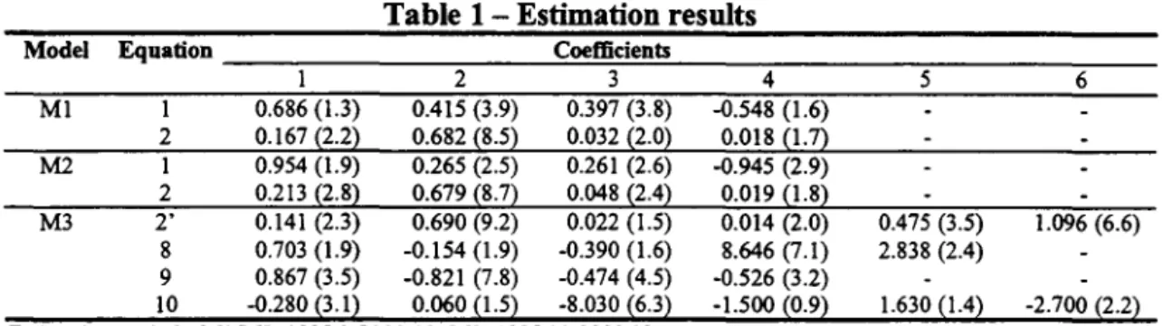
The estimated coefficients are shown in Table 1. We estimated by SURE equations (1) and (2) for models 1 and 2, and equations (2'), (8), (9) and (10) for Model 3.

6 D5 is a durnrny variable with value 1 in 1996.3, 1996.8, 1997.2, 1997.8 and 1998.8 and zero otherwise;

it refers to periods ofunusually large reductions in the inflation rate within the fixed exchange rate regime subsample 1995.11-1998.12. D6 is a dummy variable with value 1 in 1999.7, 1999.10 and 2000.7 and zero otherwise; it refers to periods of unusually large increases in the inflation rate within the floating exchange rate regime subsample 1999.1-2000.12.

7 We used a Lagrange-multiplier test to test for residual autocorrelation and Chow l-step ahead and

Table 1- Estimation results

Model Equaüon Coeflicients

1 2 3 4 5 6

MI 1 0.686 (1.3) 0.415 (3.9) 0.397 (3.8) -0.548 (1.6) 2 0.167 {2.2} 0.682 {8.5} 0.032 {2.0} 0.018 {1.7}

M2 I 0.954 (1.9) 0.265 (2.5) 0.261 (2.6) -0.945 (2.9) 2 0.213 {2.8} 0.679 {8.7} 0.048 {2.4} 0.019 {1.8}

M3 2' 0.141 (2.3) 0.690 (9.2) 0.022 (1.5) 0.014 (2.0) 0.475 (3.5) 1.096 (6.6) 8 0.703 (1.9) -0.154 (1.9) -0.390 (1.6) 8.646 (7.1) 2.838 (2.4)

9 0.867 (3.5) -0.821 (7.8) -0.474 (4.5) -0.526 (3.2)

lO -0.280 ｰＮｬｾ＠ 0.060 ｾＱＮＵｾ＠ -8.030 ｾＶＮＳｾ＠ -1.500 ｾＰＮＹｾ＠ 1.630 ｾＱＮＴｾ＠ -2.700 ｾＲＮＲｾ＠

Estimation period - MIIM2: 1995.1-2000.12; M3: 1995.11-2000.12 Estimation method - SURE (t-statistics in parentheses)

Coefficients in the potential GDP equations were selected so as to maximize 6-step-ahead predictive power. Using the sample period from 1991.1 to 2000.12 we estimated the following coefficients:

8

=

0.3,l/J

=

0.92 .

Estimation results are not particularly good, as we note some rather low t-statistics and the need for several dummy variables in Model 3. However, our basic selection criteria are satisfied: all key coefficients have the expected signs and we do not reject either the absence of residual autocorrelation or parameter constancy.8 Appendix 2 presents graphs with Chow tests for each model.

It is interesting to compare the estimated coefficients for the real interest rate in equation (1) and for the output gap in equation (2) under models 1 and 2. As expected, both coefficients are smaller in Model 1, in which the output gap is derived from a deterministic potential product. For obvious reasons, these results wil1 have important implications for the calculation of the optimal policy rule in the next section.

3. Calculation of the optimal monetary policy rule

The literature usua1ly characterizes monetary policy as the management of a short-term instrument, such as the monetary base or interest rates, \\ith the objective of minimizjng expected deviations of inflation and the output gap from prespecified target leveIs (see, inter alia, Svensson (1996, 1997), Blinder (1998), Walsh (1998)). A typical problem for the policymakers would therefore be to

minz G =

Eo{Lt=O

(yt-Y*t)2

subject to Yt=AYt.l+BZt-l+ ｾＫｾ＠ ｾＭＨｏＬｓＩ＠

(14)

where y are target variables with target leveI y*, Z is a vector of control variables, a is a vector of aggregate effects from exogenous variables, e is a vector of stochastic shocks and A and B are non-stochastic parameter matrices.9 It is possible to show that the solution to this linear-quadratic problem is a linear deterministic function of the target variables (Chow, 1975):

8 According to the l-step Chow tests we might reject pararneter stability for a couple of periods, but we

believe this may be due to the presence of outliers.

9 Note that this is a quite general problem, as difference equations of any order may be reparameterized as

(15) This is a remarkable result known as the certainty equivalence principie: the solution to an optimal control problem in a stochastic framework may be obtained analytically and is identical to the one that would be obtained in a similar model without the stochastic termo Function (15) is called the optimal reaction function (RF).JO

It is c1ear that given the model parameters C=(A,B) we may calculate the parameters in the reaction function, FIe. However, model parameters are usually estimated, so that we may only know their probability distribution C-N(

ê

,W). In this case, the policymakers problem is to

(16)

ｾＭＨｏＬｓＩ＠ , (A,B)=C-N(

ê

,W)

In this new problem the presence of multiplicative uncertainty implies that certainty equivalence no longer holds, but we may still calculate a linear optimal reaction function, as shown by Chow (1975).

Following Chow (1975), we now show how to calculate the optimal reaction function for problems (14) and (16) in turno Letp be a discount factor and R be a weight matrix that determines the relative importance of each endogenous variable's squared deviations from target. R is isually taken to be diagonal. The loss function may be decomposed in a deterministic part (K) and a stochastic part (V) defined below:

K = Lpt {(E(Yt)-y*)'R(E(Yt)-Y*) V = (Yt-E(Yt»'R(Yt-E(Yt»}

P(z)= Eo{Lpt (Yry*)'R(Yt-Y*)}

=

K(z)+Eo V(z)

(17) (18) (19) The oprimal reaction function for problem (14) with known parameters is given by the terminal condition for the value function ＨｐｾｒＬ＠ ｨｾ＠ Ry*) and by the Riccati equations. These equations are solved iteratively from the last to the first period and give us each period's value function (Pt.ht) , which is used in the calculation of the reaction function. As the econometric model may inc1ude rime-dependent exogenous variables (3.t), we use the indicated non-stationary solution. Nonetheless, the reported oprimal reaction function refers to the initial period.

Pt-1

=

R + pA'R A - pA'Pt B (B'PtBf1B'PtA

ht-l

=

R y* -(A + BFt) '(Pt3.t -

ht)

Zt

= -

(B'PtBf1B'PtA Yr (B'PtBf1B' (Ptat -

ht)

=

Ft Yt +

ft

(20) (21) (22)

For problem (16) with unknown parameters we use the same terminal condition (P-r=R. h-r=Ry*) and the expected value of terms in brackets in the equations below are obtained by simulation. We generate 1000 realizations ofmodel parameters C-N(ê ,W) using the estimated distribution of each macroeconomic model in Section 2. Once again, we use the non-stationary solution and the optimal reaction function refers to the initia! period.

Et{Pt-d

=

R + _{p Et {A'R A - pA'Pt B (B'ptBr1B'ptA}} (23) Et{ht-l}

=

R y* - Et{ (A

+

BF) '(Ptli( - ht)} (24) Zt = - {Et(B'ptB)r1Et(B'ptA) -{Et (B'PtB)ri Et{B'(Ptllt - ht)} = FtYt +

ft

(25) The above procedures allow us to calculate the optimal reaction function for each one of the models presented in Section 2. But we do not know which empírical model provides the best approximation to the ''true'' model and are therefore uncertain as to which policy mIe should be regarded as the best overall mIe.

One way to approach this question is to investigate each mIe's robustness by calculating the policymaker's loss under each model (m) given each reaction function (n), i.e. PrnlFn. The policymaker's loss may be obtained by simulating 1000 realizations of model parameters C-N( C ,W) and disturbances ｾＭＨｏＬｓＩＬ＠ which generate trajectories for (y,z), and then using expressions (17)-(19) to calculate the expected loss.

In the following exercises we assume that policymakers target a 0.487% monthly inflation rate (corresponding to 6% per year) and a zero monthly output gap, with equal weights. Results would be obviously different if we adopted some other criterion, such as to target average inflation over one year.

In all cases we assume the discount factor to be 1 and present results for the deviation ofE(y), given by K, and the deviation ofy, given by P.

3.1 Results

Table 2 presents the optimal reaction function coeflicients for each model estimated in Section 2, both under the hypothesis of purely additive uncertainty, i.e. known parameters [FIE(C)], and under the hypothesis of additive and multiplicative uncertainty, i.e. unknown parameters [Flc]. From this table we may draw some very interesting conclusions.

First, comparison between response coeflicients in FIE(C) and in FIC within each model shows that the presence of multiplicative uncertainty should make policymakers react less aggressively to the economy's state variables, as suggested by Brainard's "conservatism principIe". However, this effect seems to be relatively small in most cases, which is consistent with the findings in Peersman and Smets (1999), Estrella and Mishkin (1998) and Rudebusch (1999), inter alia.

Model 2. In part, this may be explained by the different potential GDP definitions used in MI and M2. In Model I, the use of a deterministic potential output im.plies: (i) an output gap with larger variance; (ü) smaller effects of monetary policy on the output gap; (iü) smaller effects ofthe output gap on inflation (see Table I). As a consequence, optimal policy must respond more aggressively to the output gap in order to keep both the output gap and inflation under controI.

Third, it is interesting to analyze the coefficient on the lagged nominal interest rate, which enters the optimal reaction function through equation (4) and may be interpreted as a measure of interest-rate smoothing - the higher the coefficient, the more sluggish interest rate movements would tend to be. According to our findings, this coefficient is very small in all cases, especially in models I and 2 (when they are nearly zero); we therefore conc1ude that according to our empirical models optimal policy should incorporate very little interest rate smoothing.

Table 2 - 0l!timal reaction functions

Model RF ÂC & &.1 ÂX 7t 7t·1 7t·2 U QI T·I

Ml FIE(C) 0.359 0.330 0.330 0.760 0.724 0.000

Fie 0.352 0.330 0.329 0.568 0.540 0.000

M2 FIE(C) 0.350 0.330 0.330 0.283 0.278 0.000

Fie 0.346 0.330 0.329 0.250 0.243 0.000 M3 FIE(C) 0.828 0.180 -0.480 0.700 0.256 0.311 0.311 0.979 0.000 0.058

Fie 0.750 0.160 -0.439 0.637 0.262 0.313 0.313 0.887 0.000 0.053

The following results refer to the application of the optimal rules derived under the hypothesis ofboth additive and multiplicative uncertainty, i.e. [Flc].

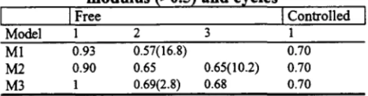
Table 3 presents each model's largest characteristic roots before applying the optimal policy rule (the "free"case) and after applying it (the "controlled" case). We can see that the system is unstable in the absence of the policy rule but becomes stable when the latter is operative. As expected, the policy rule stabilizes the system.

Table 3 - Characteristic roots for models 1 to 3:

Model

MI

M2 M3

modulus (>0.5) and cycles

I

Free

I

ControIled

1 2 3 1

0.93 0.57(16.8) 0.70 0.90 0.65 0.65(10.2) 0.70 0.69(2.8) 0.68 0.70

* Cycles in parentheses (in months)

M2 M3

Mean

TR RFIM1 RFIM2 RFIM3

1.16 1.00 1.36 3.35

1.04 2.65 1.00 2.69 2159 2.41

1.27 7.09 2.33 1.00 3.39 113 6.88 5.11

• Value for the 95íh percentile ofthe loss distribution function

Given any specific model, we note that the adoption of the optimal rule calculated from some other model always leads to very poor results in terms of expected loss. The additionalloss caused by using the ''wrong'' optimal policy ranges from 36% in the best case (use ofRFIM2 in Ml) to 600% in the worst case (use ofRFIMl in M3).

On the other hand, the performance ofthe simple Taylor role across models 1-3 is quite robust. In every model, the Taylor role is ranked second, losing only to the model's own optimal rule in terms of expected 10ss. In other words, given any specific model it is always better to adopt the Taylor rule than to adopt the ''wrong'' optimal rule calculated from some other model. Even more important, the performance of this simple rule is reasonably c10se to each model' s own optimal rule; the additionalloss from using the Taylor role varies from only 4% in Mode12 to 27% in Mode13.

The Taylor rule's robustness is even more remarkable when we consider values "under risk", i.e. under particularly unfavourable realizations from the model's probability distribution.ll In such circumstances, the Taylor rule's performance deteriorates much less than the optimal rules. Under models 1 and 3, the Taylor role performs even better than those mode1s' own optima1 roles. This is a very interesting result: even within a specific model, the adoption of the optima1 role does not guarantee the best performance in practice. The reason for this should be c1ear: the optimal rule is calculated so as to minimize expected 10sses, but the probability distribution for 10sses may be such that in practice other rules may provide better performance, as Tab1e 4 shows.

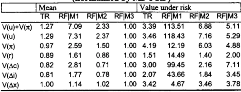
Tab1es 5 to 7 give a more detailed account ofthe results from our exercise. In each tab1e, we report the variances of the output gap, inflation and interest rates calculated in a specific model under each possib1e policy rule. We also report variances of consumption, investment and net exports for Mode1 3. Note that the first line in each of these tab1es is total welfare 10ss and is therefore the same as the corresponding line in Tab1e 4.

11 We take the 95th percentile of the loss probability distribution function as a proxy for ''value under

Table 5 - Variance ofE(Y) in Ml under Ml's and M2's RF

V(u)+V(n) V(u) V(n) V(r)

(normalized by Ml 's RF)

I

Mean

I

Value under risk

I

TR RFIM1 RFIM2 TR RFIM1 RFIM2

1.16 1.00 1.36 3.35 9.42 4.40

1.18 1.00 1.38 3.56 10.35 4.70

0.90 1.00 1.02 3.15 4.08 3.96

0.87 1.00 0.81 1.47 2.31 1.38

Table 6 - Variance ofE(Y) in M2 under Ml's and M2's RF

V(u)+V(n) V(u) V(n) V(r)

(normalized by M2's RF)

I

Mean

I

Value under risk

TR RFIM1 RFIM2 TR RFIM1

1.04 2.65 1.00 2.69 2159.07

1.06 0.92 1.18

2.79 1.33 1.70

1.00 2.84 2356.90

1.00 2.67 55.86

1.00 1.75 461.81 RFIM2

2.41 2.52 2.98 1.49

Table 7 - Variance ofE(Y) in M3 under each model's RF

IMean

{normalized ｢ｾ＠ M3's RF)

I Value under risk

TR RFIM1 RFIM2 RFIM3 TR RFIM1 RFIM2 RFIM3

V(u)+V(n) 1.27 7.09 2.33 1.00 3.39 113.51 6.88 5.11

V(u) 1.29 7.31 2.37 1.00 3.46 118.43 7.16 5.29

V(n) 0.97 2.59 1.50 1.00 4.19 12.19 6.03 4.88

V(r) 0.89 1.61 0.86 1.00 1.51 14.49 1.40 2.00

V(Ác) 0.82 2.81 0.71 1.00 3.00 99.45 2.16 7.11

V(Ái) 0.81 1.77 0.78 1.00 2.07 43.66 1.84 3.45

V(ÁX) 1.00 1.14 1.02 1.00 3.42 4.67 3.46 3.78

4. Conclusion

Based on three versions of a small macroeconometric model for Brazil, this paper has provided empirical evidence on the relation between uncertainty and monetary policy rules and on the robustness of optimal and simple rules across different model specifications. Our main findings were as follows:

(1) The presence of multiplicative uncertainty should make policymakers react less aggressively to the economy's state variables, as suggested by Brainard's "conservatism principIe", although this effect seems to be re1atively small. (2) Oprimal policy should respond more aggressively to the output gap when

potential output is deterministic than when it is stochastic.

(3) The simple Taylor rule is relatively robust across model specifications, whereas the optimal rules derived from each model perform very poorly under alternative models.

(4) Even within a specific model, the Taylor rule may perform better than the optimal rule under particularly unfavourable realizations from the policymaker' s loss distribution function.

References

Andrade, l and Divino, lA. (2000) Optimal rules of monetary policy for Brazil, Mimeo.

Ball, L. (1999) Efficient rules for monetary policy, /nternational Finance, 2: 63-83. Bemanke, B.S., Laubach, T., Mishkin, F.S. and Posen, A.S. (1999) /njlation Targeting: Lessons from the /nternational Experience, Princeton University Press.

Blinder, A. (1998) Central Banking in theory and practice, MIT Press.

Bogdanslá, J., Tombini, A., Werlang, S. (2000) Implementing inflation targeting in

Brazil, Working Paper Series 1, Central Bank of Brazil.

Brainard, W. (1967) Uncertainty and the effectiveness of policy, American Economic Review, Vo1.57, 411-425.

Chadha, lS. and Schellekens, P. (1999) Monetary Policy Loss Functions: Two Cheers for the Quadratic, DAB Working Papers, Department of Applied Economics, University of Cambridge.

Chow, G. (1975) Analysis and Control of Dynamic Economic Systems, John Wiley and Sons, New Y ork.

Drew and Hunt (2000) Efficient simple policy rules and the implications of potential output uncertainty, Journal ofEconomics and Business, 52: 143-160.

Estrella, A. and Mishkin, F. (1998) Rethinking the role of the NAIRU in monetary policy: Implications of model formulation and uncertainty, Federal Reserve Bank of New York Research Paper 9806.

Hall, S., Salmon, c., Yates, T. and Batini, N. (1999) Uncertainty and simple monetary policy rules: An illustration for the United Kingdom; Working Paper Series no. 56, Bank of England.

Levin, A., Wieland, V. and Williams, J.c. (1999) Robustness of simple monetary policy rules under model uncertainty, in John B. Taylor, ed., Monetary Policy Rules, Chicago Press.

Levin, A., Wieland, V. and Williams, lC. (1999) The performance of forecast-based monetary policy rules under model uncertainty, Mimeo, Board of Govemors of the F ederal Reserve System.

Martin, B. and Salmon, C. (1999) Should uncertain monetary policy-makers do less? Bank of England Working Paper.

McCallum, B. (1999) Recent developments in the analysis of monetary policy roles, Federal Reserve Bank ofSt. Louis Review, 81(6).

McCallum, B. (2000) The present and future of monetary policy roles, NBER Working Paper 7916.

Orphanides, A. (1998) Monetary policy evaluation with noisy information, FEDS Working Paper 1998-50.

Rudebusch, G. (1998) Is the Fed too timid? Moneta.ry policy in an uncertain world, Federal Reserve Bank of San Francisco Working Paper, forthcoming in the Review of Economics and Statistics.

Rudebusch, G. and Svensson, L. (1998) Policy rules for inflation targeting; Seminar Paper No. 637, Institute for International Economic Studies, Stockholm University. Sack, B. (1998) Does the FED act gradually? A V AR analysis, FEDS Working Paper 1998-17.

Sargent, T. (1999) Discussion of "Policy rules for open economies" by Laurence Ball, in J.B. Taylor, ed., Monetary Policy Rules, Chicago Press.

Shuetrim, G. and Thompson, C. (1999) The implications of uncertainty for monetary policy, Reserve Bank of Australia, Research Discussion Paper 1999-10.

Simon, H. (1956) Dynamic Programming under uncertainty with a quadratic criterion function, Econometrica, XXIV, 74-81.

Smets (1998) Output gap uncertainty: Does it matter for the Taylor rule?, Mimeo, European Central Bank.

Svensson, L. (1996) Inflation forecast targeting: Implementing and monitoring inflation targets; Working Paper Series no. 56, Bank ofEngland.

Svensson, L. (1997) Inflation targeting: some extensions; Seminar Paper No. 625, Institute for International Economic Studies, Stockholm University.

Svensson, L. and Woodford, C. (2000) Indicator variables for optimal policy, NBER Working Paper 7953.

Swanson, E. (2000) On signal extraction and non-certainty equivalence in optimal monetary policy rules, Working Paper, Federal Reserve Board.

Taylor, J.B. (1993) Discretion versus policy rules in practice, Carnegie-Rochester Conference Series on Public Policy 39, 195-214.

Tetlow, R.J. and von zur MuehIen, P. (1999) Can model structure uncertainty imply policy attenuation?, Mimeo, Federal Reserve Board.

Theil, H. (1957) A note on certainty-equivalence in dynamic planning, Econometrica, XXV, 346-349.

Walsh, C.E. (1998) Monetary Theory and Policy, MIT Press.

Appendix 1

Data description and graphs

Variable Name SourceJDefmition

1t Inflation Monthly percent change in the broad consumer price index (IPCA) from IBGE

r Nominal Monthlyaverage SELIC ovemight interest rate from Brazil's Central Bank interest rate

d Nominal Percent change in the monthly average rate from Brazil's Central Bank exchange rate

depreciation

y GDP Seasonally adjusted monthly chained index series at 1990 Reais; raw data are from IBGE

y* Potential Calculated from equations (6) or (7) in the text GDP

u Outputgap Calculated from equation (5) in the text

i Investment Seasonally adjusted monthly index series from IPEA at 1990 Reais

c Consumption Seasonally adjusted monthly index series at 1990 Reais ca1culated by the authors as follows: first, we calculated nominal monthly GDP based on IBGE's monthly chained index series and on FGV's general price index (lGP-DD, using a factor to make the series consistent with the annual National Accounts figures; second, we calculated nominal investment based on IPEA's monthly index series and on price indices for construction (lNCC from IBGE) and for machinery and equipment (lP A-máquinas e equipamentos from FGV), also using a correcting factor to make the series consistent with the National Accounts; third, we calculated net exports of goods and non-factor services based on Balance ofPayments and exchange rate data from the Central Bank, again making the series consistent with the National Accounts; fourth, we calculated nominal consumption as a residual from C = Y - I - (X-M); finally, we calculated real consumption at 1990 Reais by using the IPCA as the consumption deflator and making the series consistent with the National Accounts.

Graphs

1995 2000 1995

ＱＳＰｾＭ

Y

I

ｾ＠

/

125

l

V

r-}r

110[L-_-'

ＱＲＰｾ＠

(1

ｾ＠

115

k

;1

1

100

90

1995 2000

us: u with detenninistic potential output ud: u with stochastic potential output

1995

2000 1995 2000

27.5

25

22.5

Appendix 2

Parameter constancy tests for models 1 to 3

Modell: l-step ahead (lup) and break-point (Ndn) Chow tests

2.5

l-lupCHOWs 5%

II

2

1\

1.5 I1

1'

ｾ＠ ｉｾ＠

1\ . I

i I i \ ,\

r

II

\}:

! , ; \

.5

ｾ＠

IV

I

ｾｬ＠

1996 1997 1998 1999 2000 2001

1 ₁ l<ldu eool'ls ｾＬｯ＠

ｾ｜＠

.75

I

.5

,25

/

/ /

1996 1997 1998 1999

Model2: l-step ahead (lup) and break-point (Ndn) Chow tests

2

f

1-

lupCHOWs

1.5

5%

1996 1997 1998 1999

I-NdnCHOWs - 5%

.75

.5

.25

1996 1997 1998 1999

Model3: l-step ahead (lup) and break-point (Ndn) Chow tests

ｂｾｾｾ］ﾷＺＮＧ＠ ｾ＠

'"

W,rrJ H::NRiQUE SIMONSEN

ｦｕＺｾ］＠

t,:::Ao

G::TUUO VARGAS

I i I

v-

_\ ! _! 2000

!

.1\

!!

!I

I i \

1\ '! I

2000

ｾ｜＠

I

I \ \ !

l"\

\ 2000

\

ｾ＠

l-lupCHOWs 5% .75

i

1\

.5

1

1\

I \

I

\

I

.25

I

V

ｾ＠

I

/ rvv

1997 1998 1999 2000 2001

I-NdnCHOWs 5% .75

.5

_I

.25

Mean TR 0.64

M2 0.97

M3 1.36

Mean TR V(u)+V(1t) 0.64

V(u) 0.58

V(1t) 0.04

V(dr) 0.12

V(r) 3.11

Mean TR V(u)+V(1t) 0.97

V(u) 0.90

V(1t) 0.06

V(dr) 0.41

V(r) 3.61

Mean TR V(u)+V(1t) 1.365

V(Dc) 0.155

V(Di) 0.253

V(Dx) 0.127

V(1t) 0.031

V(u) 1.323

V(r) 3.039

Appendix 3

Welfare loss for models 1 to 3 under the Taylor rule and under each model's optimal reaction function

Value under risk

RFIM1 RFIM2 TR RFIM1 RFIM2 RFIM3

0.55 0.75

-

1.84 5.18 2.42

2.46 0.93 - 2.50 2008 2.24

7.61 2.51 1.07 3.64 121 7.38 5.49

in Ml under Ml's and M2's RF

Value under risk RFIM1 RFIM2 TR RFIM1 RFIM2

0.55 0.75 1.84 5.18 2.42

0.50 0.69 1.76 5.13 2.33

0.05 0.05 0.15 0.20 0.19

0.22 0.03 0.35 2.76 0.10

3.56 2.87 5.22 8.21 4.93

in M2 under Ml's and M2's RF

Value under risk

RFIM1 RFIM2 TR RFIM1 RFIM2

2.46 0.93 2.50 2008.84 2.24

2.38 0.85 2.42 2008.08 2.15

0.09 0.07 0.18 3.69 0.20

2.02 0.11 1.13 1116.78 0.31

5.19 3.05 5.33 1409.90 4.55

Value under risk

RFIM1 RFIM2 RFIM3 TR RFIM1 RFIM2 RFIM3 7.614 2.506 1.0743.638 121.97 7.385 5.489 0.533 0.134 0.190 0.570 18.895 0.410 1.351 0.553 0.243 0.3130.649 13.667 0.575 1.079

0.145 0.130 0.1270.434 0.593 0.440 0.480

0.083 0.048 0.0320.134 0.390 0.193 0.156

FUNDAÇÃO GETULIO VARGAS

BIBLIOTECA

ESTE VOLUME DEVE SER DEVOLVIDO À BIBLIOTECA NA ULTIMA DATA MARCADA

N.Cham. PIEPGE SA M838r

Autor: Moreira, Ajax R. Bello (Ajax Rey

Título: Robustness and stabilization properties of

ＱＱＱＱＱＱｾＱＱＱｾｬｬｬｬｬｮｬｬｮｬｬｭ＠

III

ＺｾｉＺＡＰＷ＠

FGV -BMHS N° Pat.:307807/02

ij

Ú

;-

ｾＱＲＴｾｾ＠

ｾ＠

r

BIBLlorC:CA MARIO 1',Ef<r,!c',- " r)":SEN