Optimization of composite catenary risers

(1)

Optimization of composite catenary risers

Rafael Fernandes da Silva

a

_{, Fábio Anderson Fonteles Teó}

ﬁ

lo

a

,

Evandro Parente Jr.

a,_*

_{, Antônio Macário Cartaxo de Melo}

a

_,

Áurea Silva de Holanda

b

a_{Laboratório de Mecânica Computacional e Visualização (LMCV), Departamento de Engenharia Estrutural e}

Construção Civil, Universidade Federal do Ceará, Campus do Pici, Bloco 728, 60440-900 Fortaleza, Ceará, Brazil

b_{Departamento de Engenharia de Transportes, Universidade Federal do Ceará, Campus do Pici, Bloco 703,}

60440-900 Fortaleza, Ceará, Brazil

a r t i c l e

i n f o

Article history: Received 6 July 2011

Received in revised form 12 April 2013 Accepted 13 April 2013

Keywords: Composite materials Marine risers Structural optimization

a b s t r a c t

The use of composite risers may offer important advantages over the use of conventional steel risers in deepwater oilfields. How-ever, the design of laminated composite risers is much more complex than the design of steel risers, due to the large number of parameters that need to be chosen to define the riser layup. This work presents a methodology for optimum design of composite catenary risers, where the objective is the minimization of cross-sectional area of the riser and the design variables are the thick-ness andfiber orientation of each layer of the composite tube. Strength and stability constraints are included in the optimization model and multiple load cases are considered. The methodology can handle both continuous and discrete variables. Gradient-based and genetic algorithms are used in the computer implementation. The proposed methodology is applied to the optimization of composite catenary risers with different water depths, liner ma-terials, and failure criteria. The numerical examples show that the proposed methodology is very robust.

*Corresponding author.

E-mail addresses:[email protected](R.F.da Silva),[email protected](F.A.F. Teóﬁlo), [email protected](E. Parente),[email protected](A.M.Cartaxode Melo),[email protected](Á.S.de Holanda).

Contents lists available atSciVerse ScienceDirect

Marine Structures

j o u r n a l h o m e p a g e : w w w . e l s e v i e r . c o m / l o c a t e / m a r s t r u c

(2)

1. Introduction

The depletion of existing reserves and the increasing demand for oil and gas have led to the search for deepwaterﬁelds and research in new technologies to make the production feasible. Fiber reinforced composite materials present several advantages for offshore applications, such as high speciﬁc strength and stiffness, high corrosion resistance, low thermal conductivity, excellent damping properties, and high fatigue resistance.

These favorable properties have motivated the oil industry to use composite materials in different offshore applications[30], including risers[22,29,32,34]and stress joints[21]. The reduced weight obtained by the use of composite risers in replacement to steel risers can be substantial, leading to a signiﬁcant reduction of top tension requirements, which allows the use of simpler and smaller tension mechanisms and smaller platforms[22,30,34].

This work addresses the use of Composite Catenary Risers (CCR) as an alternative to Steel Catenary Risers (SCR) for deepwaterﬁelds. The design of laminate composite structures involves a large number of parameters, including the number of layers and the material, thickness, andﬁber orientation of each layer. Thus, the use of the conventional trial-and-error strategy is not adequate and optimization techniques have been widely used in the design of laminated composite structures[15].

The use of optimization techniques in the design of marine risers is recent, but the number of applications has been steadily growing. Different optimization algorithms as Sequential Quadratic Programming (SQP)[18], Simulating Annealing (SA)[35], Artiﬁcial Immune Systems (AIS)[37], and Particle Swarm Optimization (PSO)[25]have been used for SCR design. Genetic Algorithms (GA) have also been used in the design of SCRs in free hanging and lazy wave conﬁgurations[19,35,37,40], since

they are very robust, easily deal with discrete variables, non-continuous and non-differentiable functions, and avoid getting trapped by local minima.

This work presents a methodology for optimum design of Composite Catenary Risers in free hanging conﬁguration. The design variables are the thickness andﬁber orientation of each layer. The

objective is to minimize the cross-sectional area of the riser joint, considering strength and stability constraints. It is important to note that to the best of the authors’knowledge this is theﬁrst work dealing with optimization of composite catenary risers.

This paper is organized as follows. Section2presents the main components of composite riser joints and discusses the design of composite risers. Section3addresses the structural analysis of composite catenary risers and Section 4 describes the optimization model, including the design variables, objective function, and constraints. Section 5 presents the numerical examples. Finally, Section6

presents the main conclusions.

2. Composite catenary risers

Composite risers are assembled using a series of joints connected to each other by appropriate connections. Riser joints can have short lengths (10–25 m), intermediate lengths (100–300 m), or long

lengths (>300 m)[24]. Top tensioned composite risers for drilling and production generally use short

joints, but intermediate and long joints may be better suited for catenary risers. There is also potential for the development of spoolable composite risers without intermediate joints, simplifying the transportation and installation[28]. Composite riser joints are composed generally by three elements: liner, composite tube, and terminations[2,23].

(3)

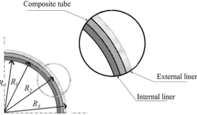
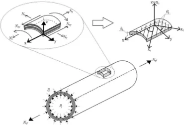
The composite tube is the main structural element of the riser joint. It is constituted by various layers ofﬁbrous composite materials. Carbon and glassﬁbers are the most used in composite risers, while the matrix is usually a polymeric resin (thermoset or thermoplastic). The material, thickness, and

ﬁber orientation of each layer should be chosen in order to provide sufﬁcient strength and stiffness to the riser joint. A scheme of the riser wall is depicted inFig. 1.

The joint terminations are metallic pieces composed of two parts: the metal-to-composite interface (MCI) and the connections. The MCI transmits the stresses from the composite tube to the metallic connectors, while the connections are responsible to join the composite joints, assembling the riser. The design of terminations (MCI/connections) is not addressed here, since the major concern of this work is the design of the composite tube.

3. Global–local analysis

Composite structures are generally analyzed by theﬁnite element method (FEM) using solid or shell elements, since these elements allow the consideration of the material, thickness, and orientation of each ply. The use of shell or solid elements yields the stresses and strains in each ply, which are used to verify the design safety using an appropriate failure criterion. However, the modeling of risers using solid or shell elements leads to a prohibitively high computational cost for practical applications. Thus, the analysis of composite risers is carried-out in two levels: global and local. This approach is generally used forﬂexible risers[39]and has also been recommended for composite risers[12,17,23].

In this approach, the global analysis of the riser is generally carried-out using beam elements, allowing the consideration of dynamic and nonlinear effects due to external loads,ﬂoater offset, currents, and waves. The global analysis yields the displacements and stress resultants (axial force, bending and torsional moments) along the riser. However, the use of beam elements does not allow the direct computation of stresses and strains at each ply of the composite tube. Therefore, the stress resultants calculated in global analysis at critical joints are used as input data for local analysis. The local analysis should be carried-out using analytical expressions orﬁnite element (shell or solid) models, since these elements allow the computation of stresses and strains at each ply, as required by the failure criteria of composite materials.

3.1. Global analysis

Since the main objectives are to study the inﬂuence of the riser parameters over the optimum

design and to assess the robustness and efﬁciency of the optimization procedure, in the current work the global analysis is performed using an analytical catenary solver, which is much faster than the FEM and provides representative results. Simpliﬁed analyses methods have also been used in other

for-mulations for optimum riser design, as catenary solvers[25,37], staticﬁnite element analysis[1,18,19], and linearized frequency-domain analysis[35].

The riser axial forces are estimated considering the riser as an inextensible cable subjected to a vertical load distributed along its length[33]. The dry weight of the riser per unit length (wdry) is given

(4)

by the sum of the weight per unit length of the terminations (wend), the internal and external liners (wil

andwel), and the composite tube (wc):

w_dry ¼

d

_endw_endþ ð1

d

_endÞðwcþw_ilþw_elÞ

w_end ¼

g

_end

p

h_ðR₀þh_endÞ2 R₀2i; wc ¼

g

_c

p

hR2₂ R2₁i

w_il ¼

g

_il

p

h_R2

1 R20

i

; w_el ¼

g

_el

p

h_R2

3 R22

i

(1)

where

d

endis the ratio between the length of terminations and the length of the joint and

g

end,

g

c,

g

il,

and

g

el, are the speciﬁc weight of the materials employed in the terminations, composite tube, internal

and external liner, respectively. The radiuses of each concentric tube (inner liner, composite tube and external liner) are depicted inFig. 1.

The weight of the internalﬂuid per unit length (wﬂ) is added to the dry weight, while the weight of

the displaced water per unit length (wbuo) is subtracted to provide the effective or apparent weight

(wef) of the riser per unit length:

w_ef ¼w_dryþw_fl w_buo

w_fl ¼

g

_fl

p

R2₀; w_buo ¼

g

_wat

p

R2₃ (2)

where

g

ﬂand

g

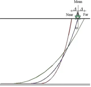
watare the speciﬁc weight of the internalﬂuid and sea water.

The riser geometry and effective axial force (Nef) are computed by the catenary solver from the

effective weight (wef), top angle with the vertical (

a

), and sea depth for the mean conﬁguration. At near

and far conﬁgurations theﬂoater offset (

D

) is applied to the mean conﬁguration, as depicted inFig. 2.

3.2. Local analysis

In the present work, the classical lamination theory (CLT) is used to perform the local analysis of critical sections of the riser. The internal liner and the composite tube are considered to be perfectly bonded and are analyzed as a single structural system. The external liner is neglected in the local analysis.

The model used in the local analysis is shown inFig. 3and consists of a cylindrical structure composed ofNlayers. Theﬁrst layer represents the internal metallic liner and the remainderNclayers

constitute the composite tube. The structure is subjected to axial forceNef(obtained from the global

analysis), internal pressurepiand external pressurepe. The thickness of thekth layer is denoted byhk.

(5)

The structure is referenced in a global coordinate system (x,y,z) with origin at the shell middle surface wherexis the longitudinal,yis the circumferential, andzis the radial direction. Theﬁber orientation of thekth layer (

q

k) deﬁnes a local coordinate system (x1,x2,x3) wherex1is parallel to theﬁbers,x2is

perpendicular to theﬁbers, andx3is perpendicular to the lamina. The in-plane (membrane) forces in

the riser wall are calculated using the theory of thin-walled tubes:

Nx ¼ Ntw 2

p

_R ¼

g

_F

b

N_efþp_i

p

_R2

0 pe

p

R22

2

p

R Ny ¼

g

FðpiR0 peR2Þ

Nxy ¼0

(3)

In this expression,Ntwis the true wall force[33],Ris the mean radius of the structural system formed by internal liner and composite tube,

b

is an ampliﬁcation factor used to account for the environment

loads as well as bending, torsion and dynamic effects, and

g

Fis the load factor used to compute the

design forces[11,12]. It is important to note thatNxy¼0, since torsion is not considered by the catenary

solver.

Using the CLT[10,16,27], the generalized stress–strain relationship to laminated composites can be

written as:

_N

M

¼

_A _B

B D

ε_m

k

(4)

whereAis the membrane (or extension) stiffness matrix,Dis the bending stiffness matrix, andBis the

bending-extension coupling stiffness matrix,ε_mis the vector of membrane strains, and

k

is the vector of

curvatures of the laminate. The resultant forces and moments are symbolized byN¼ fNxNyNxygtand

M¼ fMxMyMxygt, respectively.

In the present work, the riser is subjected only to axisymmetric loads (M¼0). Furthermore, there is no extension-bending coupling (B¼ 0) due to the axisymmetric characteristic of the riser cross-section. Thus, the stresses at thekth layer in the material coordinate system

s

k

1 ¼ f

s

k1

s

k2

s

k12gt are

computed from:

s

k

1 ¼QkTkA 1N (5)

whereQkis known as the reduced stiffness matrix[16]andTkis the transformation matrix computed from the director cosines of the local axes with respect to the global axes[9].

(6)

3.3. Failure criteria

In the present work, the von Mises failure criterion is employed to verify the strength of the metallic liner, while the strength of the composite layers are checked using the maximum stress or Tsai-Wu failure criteria. The safety factor of the internal liner (SFil) is computed as

SFil¼

_s

fy vm

s

vm ¼

ffiffiffiffiffiffiffiffiffiffiffiffiffiffiffiffiffiffiffiffiffiffiffiffiffiffiffiffiffiffiffiffiffiffiffiffiffiffiffiffiffiffiffiffiffiffiffiffiffiffiffiffiffiffiffiffiffiffiffiffiffiffiffiffiffiffiffi

s

il x

2

_s

_il

x

s

ilyþ

s

ily 2

þ3

s

il yx

2 q

(6)

wherefyis the yielding stress of the metallic material employed in the liner,

s

vmis the von Mises stress,

and

s

ilx,

s

ilyand

s

ilxyare the stresses in the liner, referenced at the global coordinate system.

Using the maximum stress criterion, the safety factor of thekth composite layer (SFk) is given by

SFk ¼MIN

SFX

k; SFYk; SFSk SFX k ¼ 8 > > > > > < > > > > > : Xt

s

k₁

; if

s

k

10

Xc

s

k₁

; if

s

k₁0

SFY k ¼ 8 > > > > > < > > > > > : Yt

s

k₂

; if

s

k₂0

Yc

s

k₂

; if

s

k₂0

SFS k ¼

S₁₂

s

k₁₂

(7)

whereXt,Xc,YtandYcare the tensile and compressive strength of the material parallel and

perpen-dicular to theﬁber orientation, whileS12is the in-plane shear strength of the material.

Alternatively, the safety factor of thekth layer of the composite tube (SFk) can be computed using

the Tsai-Wu criterion:

SFk ¼

bþpffiffiffiffiffiffiffiffiffiffiffiffiffiffiffiffiffib2þ4a

2a (8)

where

a¼F11

s

k 1

2

þF22

s

k 2

2

þ2F12

s

k1

s

k2þF66

s

k 12

2

b¼ F1

s

k1þF2

s

k2

F₁ ¼ 1

Xt 1 Xc; F2 ¼

1 Yt

1 Yc; F11 ¼

1 XtXc

F₂₂ ¼ 1

YtYc; F12 ¼ 1 2

ffiffiffiffiffiffiffiffiffiffiffiffiffiffi

F₁₁F₂₂

p

; F₆₆ ¼ 1

S2₁₂

(9)

(7)

SFc ¼MIN_kNc_¼1ðSFkÞ (10)

The matrix cracking can be an accepted failure mode in composite risers, since the liners ensureﬂuid tightness. Thus, a more complex approach based on a progressive failure analysis could be used to evaluate the riser safety factor[12]. However, in order to obtain a conservative design with a small computational cost, the simpler FPF approach was adopted in this work.

3.4. Stability

Thin-walled structures subjected to compressive stresses may collapse due to loss of stability at load levels well below the material strength. Hoop buckling is the local buckling of the tube wall (shell buckling) caused by the compressive stresses generated by external pressure. Hoop buckling is a major concern for deepwater risers and pipelines due to the high hydrostatic pressure, especially when the riser is empty and there is no internal pressure.

The critical pressure of long orthotropic cylindrical shells[12,38]can be computed from:

pcr ¼ 3

R3 D22 B2₂₂ A₂₂

!

(11)

whereA22,B22, andD22are elements of theA,B, andDmatrices, Eq.(4), in the hoop direction. It should

be noted thatB22¼0 for symmetric laminates. Finite element analyses of perfect and imperfect

cy-lindrical shells with different lengths and composite layups subjected to external pressure showed that Eq. (11) yields good results for long shells, such as composite riser joints[36]. Furthermore, the buckling pressure of short cylinders is higher than the values given by Eq.(11).

It is well known that unavoidable geometric imperfections reduce the load carrying capacity of compressed shells due to the geometric nonlinear effects. Therefore, the collapse pressure (pcol) is

obtained by the following expression:

p_col ¼kppcr (12)

wherekpis a reduction factor to account for the effects of the geometric imperfections. A knockdown

factorkp¼0.75 is recommended for design purposes[12,38].

The safety factor for hoop buckling is computed by comparing the collapse pressurepcolwith the

differential pressure (pe pi) acting on the riser wall. In order to obtain a conservative design, the riser

is considered to be empty (pi¼0) and the contribution of the internal liner to the buckling pressure

(pcr) is neglected. Thus, the safety factor for buckling is computed from:

SFbck ¼

_g

pcol

Fpe (13)

4. Optimization model

This section presents the proposed optimization model for laminated composite risers. The input data of the problem includes the loads, material properties, number of layers (Nc) of the composite

tube, inner radius (R0), thickness of internal and external liners (hil,hel), ampliﬁcation factor (

b

), force

coefﬁcient (

g

F), and required safety factors. The objective is toﬁnd the best (i.e. lowest cost) laminate

that meets the strength and stability requirements of the composite riser.

4.1. Design variables

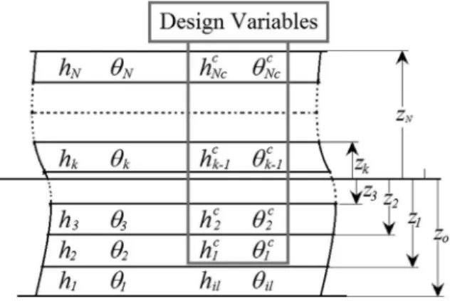
The thicknesses (hk) and theﬁber orientation angles (

q

k) of each ply of the composite tube (Fig. 4)

(8)

x¼ _h

1 h2 . hN

c=2

q

1

q

2 .

q

N

c=2t (14)

The riser weight is unaffected by the ﬁber orientations of each layer and is function of both thickness and material of each layer. The same occurs with the catenary geometry and forces, since they depend on the riser weight.

The layup is constant along the riser, since considering different properties along the riser length would increase the design space and the computational cost. Furthermore, the use of riser joints with different layups could increase the manufacture costs.

Most works dealing with optimization of laminated structures consider that design variables can only assume discrete values[13,26], but continuous variables have also been used[7]. Since the choice between continuous and discrete variables is driven mainly by manufacturing issues, both options are considered here, originating two models:continuousanddiscrete. In thecontinuous model, the design variables are limited by lower and upper bounds:

q

_min

q

_k

q

max h_minh_khmax

k ¼ 1;.; Nc

2 (15)

On the other hand, the design variables of thediscrete modelcan only assume a set of predeﬁned values (

q

_p_andhp):

q

_p _{¼ f}

_q

_min_;

_q

_min_þ

D

_q

_;

_q

_min_þ2

D

_q

_;.;

q

maxg t

hp ¼ fh_min;h_minþ

D

h;h_minþ2

D

h;.;hmaxg

t (16)

where

D

_q

_and

D

_h_{are user supplied increments.}

4.2. Objective function

Different objective functions have been used in the optimization of composite structures. In minimization problems, weight, deﬂection, and cost of composite panels[5], thickness of composite

plates[4], and the sensitivity of buckling loads due to variations in ply angles[3]have been used as objective functions. Maximization of natural frequencies and buckling loads has also been consid-ered[1].

In the present work, the cost of the riser joint is considered proportional to the volume of composite material. Thus, the objective is to minimize the cross-sectional area of the composite tube. In order to

(9)

improve the convergence of the optimization algorithm, a normalized cross-sectional area of the composite tube is used as objective functionf(x):

f x

¼ AðxÞ Amin

Amax Amin (17)

whereA(x),AminandAmaxare the current, minimum and maximum cross-sectional area of the

com-posite tube, respectively. The minimum area is obtained considering all layers of the comcom-posite tube withhk¼hminand the maximum withhk¼hmax.

4.3. Constraints

Strength and stability constraints are considered in order to ensure the structural integrity of the riser. Based on previous catenary riser analyses, two critical load cases were chosen. Load Case A corresponds to the riserfilled with internalfluid at far configuration, leading to high tension at the top riser joint. On the other hand, Load Case B corresponds to the riser without internalfluid at the near configuration, leading to high external pressure and true wall compression in the touch-down point (TDP) of the riser. In this case, a conservative design is adopted in which the small effective force at TDP and the internal pressure are neglected (Nbot_ef ¼0, pi ¼ 0) in the local

analysis.

In Load Case A, the local analysis is executed applying the effective top tensionðNtop_ef Þobtained in the global analysis and the internal pressure of theﬂuid (pi). The stresses computed from the local analysis

are used to calculate the internal liner safety factorðSFtop_il Þand the composite safety factorðSFtopc Þat the

top end. Thus, the constraints related to the liner and composite safety factors are deﬁned as:

g_iltop ¼1 SF

top il SFreq_il 0

g_ctop ¼1 SF

top c SFreq_il 0

(18)

where SFreq_il and SFreq

c are the required safety factor of the liner and the composite, respectively.

In the Load Case B, the stresses computed from the local analysis with the riser subjected only to external pressure allow the calculation of the liner and composite safety factor and the buckling safety factor at the bottom of the riserðSFbot_il ;SFbotc ;SFbckÞcorresponding to the TDP joint. The constraints

related to the liner and composite safety factors are deﬁned as:

g_ilbot ¼ 1 SF

bot il SFreq_il 0

g_cbot ¼ 1 SF

bot c SFreqc 0

(19)

The stability constraint is implemented in the normalized form:

g_bck ¼1 SFbck

SFreq_bck0 (20)

where SFreq_bckis the required Safety Factor to avoid hoop buckling as deﬁned in Section3.4.

(10)

Find x¼ nh₁ h₂ . h

Nc=2

q

1

q

2 .

q

Nc=2

ot

That minimizes f x

¼ AðxÞ Amin

Amax Amin Subjected to :

gtop_il ¼ 1 SF

top il SFreq_il 0

gtop_c ¼ 1 SF

top c SFreq

c 0

gbot_il ¼ 1 SF

bot il SFreq_il 0

gbot_c ¼ 1 SF

bot c SFreqc 0

g_bck ¼1 SFbck

SFreq_bck0

If design variables have continuous values :

q

_min

q

k

q

max

h_minhkhmax

If design va riables have discrete values :

q

_k˛_f

q

_min;

q

_minþ

D

q

;

q

_minþ2

D

q

;.;

q

maxg

h_k˛_fh_min;h_minþ

D

h;h_minþ2

D

h;.;hmaxg

(21)

Fatigue caused by environmental conditions and vortex induced vibrations (VIV) is an important issue in the design of catenary risers. However, evaluation of fatigue life requires the use of complex and costlyﬁnite element analysis in time or frequency domains. These procedures were not included in the

model to keep the computational cost low, in order to allow the use of the model in personal com-puters. As a consequence, the solution of this optimization problem should be seen as preliminary designs to be used as input for more advanced analysis procedures.

4.4. Computer implementation

The optimization model described previously was implemented in MATLAB and three different optimization methods can be used to ﬁnd a solution. The ﬁrst method uses the gradient-based

sequential quadratic programming (SQP) algorithm via thefminconroutine of the MATLAB Optimi-zation Toolbox[20]. This method can be applied to nonlinear constrained problems with continuous variables.

The second method uses the penalty function (PF) approach presented by[31]to solve discrete optimization problems using gradient-based methods. In this approach, the problem is initially solved considering that design variables are continuous. After that, the variables with non-discrete values are penalized replacing the original objective functionf(x) by the modiﬁed objective functionF(x):

FðxÞ ¼ fðxÞ þsXNd i¼1

f

i_d x ₍₂₂₎

wheresis the penalty parameter,Ndis the number of discrete variables, and

f

idðxiÞis the penalty

(11)

f

i_dðxiÞ ¼ 1₂ sin 2

p

_x

i 0:25 dijþ1þ3dij dijþ1 dij þ1

!

(23)

wheredijis thejth discrete value that theith design variable can assume. The problem should be solved

repeatedly for increasing values of the penalty parameter[31]. This strategy was combined with the gradient-based SQP algorithm. The gradients were evaluated usingﬁnite differences.

One of the main drawbacks of gradient-based optimization methods is their susceptibility to be attracted by local minima. To overcome this problem, the Multistart method[6]was adopted for both continuous and discrete problems. In this procedure,Nruninitial designs satisfying the bound

con-straints in

q

kandhkare randomly generated and used as starting points forNrunindependent

opti-mizations. In the computer implementation, the optimizations are carried-out sequentially and if the new solution has a smaller objective function value than the current best design, then the best design is updated. If a sufﬁciently high number of different starting points are used, then the best design will be close to the global optimum.

The third solution method is a genetic algorithm (GA) implemented using well-known GA libraries

[8] and integer encoding. Genetic algorithms apply concepts of genetics combined with Darwin’s

theory of evolution[14] and can be used to obtain optimum solutions of continuous and discrete problems. Since GAs are zero-order methods, they do not require the computation of the gradients of objective and constraint functions. Furthermore, the use of a set (population) of designs and the random character of GA operators (e.g. selection, crossover, and mutation) help the method to avoid being trapped by local minima andﬁnd the global minimum. On the other hand, the GA is more time consuming than the SQP method. The implemented GA for discrete problems is described below.

First, an initial population is randomly generated containingNindindividuals or candidate solutions.

Each individual is represented by an integer array (chromosome) of the design variables and has its objective function and constraints evaluated. In order to consider constraints violation, a static penalty method is used and the penalized objective function is obtained for each design, according to:

FðxÞ ¼ fðxÞ þkpX Ng

i¼1

maxðg_iðxÞ;0Þ (24)

wherekpis the penalty factor andgiis theith constraint. Then, the individuals are sorted in decreasing

order of their penalized objective function and aﬁtness score based on the rank position is assigned to each individual. Individuals with the smaller penalized objective functions have greaterﬁtness scores and more chances to survive and transmit their characteristics to next generation (iteration).

The stochastic uniform selection[8]is applied on the whole population and a group ofNsel¼CrNind

individuals (parents), where Cr is known as crossover rate, is selected to perform the crossover.

Crossover is a key genetic operator for GA convergence. This operator is sequentially applied to pairs of parents and produces two new individuals, called sons, which combine traits of both parents.

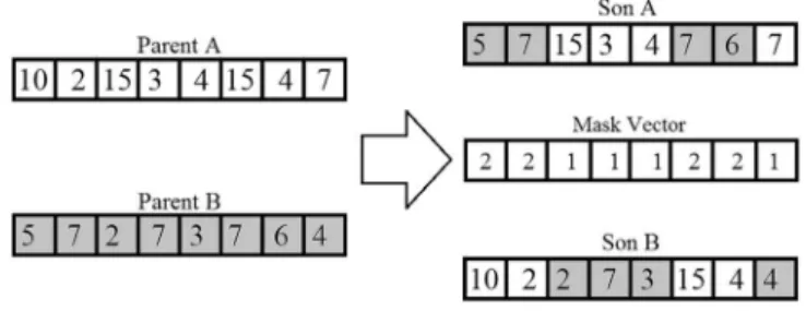
The mask crossover, depicted inFig. 5, is employed in this work. The mask is obtained by randomly generating a number (1 or 2) for each variable. If the mask value is 1, the son A inherits the design variable from parent A. Otherwise, the value comes from parent B. The opposite is applied to son B. Since two sons are created from two parents, the total number of sons is equal to the number of parents.

Even though GAs have lower probability to be trapped in local minima than gradient-based methods, premature convergence to local minima can occur. To prevent it, genetic variability has to be maintained. The mutation operator is one of the strategies used to ensure variability within the population, and it is applied in the sons generated by the crossover process. It has a low probability of occurring, symbolized byPm. For each gene of the chromosome, a random number between 0 and 1 is

generated. If such number is smaller thanPm, a random integer satisfying Eq.(16)replaces the original

gene value (Fig. 6).

Finally, a new population is formed by replacing the lesserﬁt parents with the sons. In this way, the best 1 Crindividuals of the old population are preserved (elitism selection). The process is repeated

(12)

5. Numerical examples

This section presents numerical examples in order to study the behavior of the optimization model presented in Section4. The optimum designs are achieved considering continuous and discrete design variables. The continuous problem is solved using the SQP method, while the discrete problem is solved by both PF and GA approaches described in Section4.4. The crossover rate (Cr) and mutation

probability (Pm) of the GA are set at 0.90 and 0.05, respectively. Data related to all examples are showed

inTables 1and2.

5.1. Example 1

In thisﬁrst example, the sea depth is considered as 2500 m, the top angle is 20_{, and the yield stress}

of the steel liner isfy¼448.2 MPa (API X65). The problem isﬁrstly solved adopting the Tsai-Wu failure criterion for the composite layers. The optimum designs obtained are presented inTable 3. Only one global optimum solution was found for the continuous problem. The active constraints are related to the material failure of the composite in Load Case A and the buckling constraint in Load Case B. It is important to note that this problem has multiple optimal solutions with the same cost.

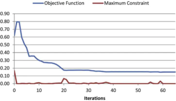
The behavior of the objective function and the maximum constraint violation in the optimization process are shown for SQP solution inFig. 7and for GA solution inFig 8. FromFig. 7it can be noted that the starting point is an unfeasible design. Initially the objective function increases while the maximum constraint violation decreases to near zero values. Then, the objective function starts to decrease.

The riser effective weight per unit length (wef) and the forces on the top of the riser are presented in Table 4for the optimum discrete solutions. The forces and weights corresponding to the continuous solutions are not presented, since they are very close to the discrete solution.

The behavior of the GA depends on the chosen parameters. The reliability (R) is the ratio of number of successful runs (Nopt) to the total number of optimizations (Nrun). The effect of population size (Nind)

and number of generations (Ngen) on the GA reliability is showed inTable 5. Clearly, the effect of the

increment on population size is more signiﬁcant than the number of generations. Maximum reliability is almost obtained withNind¼200 andNgen¼50 (R¼0.96) whereas only 76% of reliability is reached

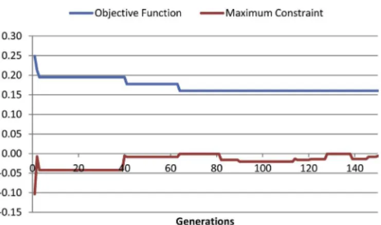
withNind¼50 andNgen¼200, both with the same number of objective function evaluations.Fig. 8

depicts GA run for a population size of 100, which shows that an optimum design can be reached with fewer generations.

Fig. 5.Crossover operator.

(13)

The reliability and computational costs for the three optimization methods are compared inTable 6. The computational cost is measured by the average number of objective function evaluations forNrun

optimizations:

N_fev ¼

PNrun

i¼1Nfevi

Nrun (25)

whereNi

fev is the number of objective function evaluations of theith optimization. The number of

function evaluations for the SQP method is different for each optimization, since it depends on the starting point. The number of function evaluations of the GA method is constant:

N_fev ¼ N_fevi ¼N_indþN_indCrNgen; i ¼1;2;.;Nrun (26)

As expected, the SQP has the smallestNfev. The GA gives the greatest computational cost, but has an

excellent reliability. Though the PF presents a small computational cost (Nfev¼1857), its reliability is

Table 1

Numerical data used in the examples.

Design parameters Internal radius [Ri] (m) 0.125

Number of layers of the composite tube [Nc] 10

Thickness of the inner (steel) liner [hil] (m) 0.006

Internal pressure [pi] (MPa) 25.0

Floater offset [Dos] 7.5% of water depth

Ampliﬁcation factor [b] 1.5

Force coefﬁcient [gF] 1.1

Thickness of the external liner [hel](m) 0.04

Speciﬁc weight–internalﬂuid [gif] (kN/m3) 7.0

Speciﬁc weight–sea water [gwat] (kN/m3) 10.05

Speciﬁc weight–external liner [gel] (kN/m3) 9.0

Fraction of the termination [dend] 0.15

Continuous variables Minimum and maximum ply thicknesses (mm) 1tk10 Minimum and maximumﬁber orientation angles 90_q_k₉₀

Discrete variables Allowable ply thicknesses (mm) {1, 2,., 9, 10}

Allowableﬁber orientation angles {0,5_,₁₀_, ., 90

_}

Constraints Required buckling safety factor½SFreq

bck 3.0

Required metallic inner liner safety factor½SFreq

il 1.5

Required composite tube safety factor½SFreq

c 3.0

Table 2

Material properties[16,27,30].

Composite E1(GPa) 137.0

E2(GPa) 9.0

G12(GPa) 7.1

y12 0.3

F1t(MPa) 1517

F1c(MPa) 1034

F2t(MPa) 34.48

F2c(MPa) 151.7

F6(MPa) 68.90

Speciﬁc weight (kN/m3₎ _15.70

Steel E(GPa) 210

y 0.3

(14)

small, showing that meta-heuristics algorithms, as GAs, are better suited to discrete optimization problems.

This example was also solved using the maximum stress criterion for the composite layers. The optimum designs are showed inTable 7. It can be noted that the composite tubes are thicker than the solution obtained for Tsai-Wu. In addition, multiple continuous solutions were found, all of them with cross-ply layups. Steel liner failure becomes active in Load Case B and buckling constraint is active only in one solution. The riser thicknesses obtained by Tsai-Wu and maximum stress have close values, but the composite safety factor in Load Case B was reduced almost by the half when the maximum stress was used as failure criterion, showing its conservative character.

It can be observed that there are not strictly active constraints in all optimum designs with discrete variables. However, the safety factors regarding to composite failure in Load Case A are very close to the minimum required values.

Table 3

Global optimum solutions for Example 1–Tsai-Wu.

Model Design variablesh(mm),q(degree) Safety factors ht(mm)

Load Case A Load Case B SFtop

il SFtopc SFbotil SFbotc SFbck

Continuous variables (SQP)

h [6.510/1.000/1.001/1.021/1.112]s 1.519 3.000 1.553 13.48 3.000 21.29 q [90.000/0.000/0.000/0.000/0.000]s

Discrete variables (PF)

h [4/1/1/2/3]s 1.594 3.238 1.524 12.77 3.172 22

q [90/90/90/0/0]s

h [5/1/1/1/3]s 1.536 3.037 1.548 13.06 3.205 22

q [90/90/0/ 50/0]s

h [5/1/1/1/3]s 1.531 3.0188 1.554 13.26 3.215 22

q [90/90/0/ 55/0]s

h [2/4/1/3/1]s 1.535 3.0166 1.563 13.21 3.243 22

q [90/90/ 55/5/5]s

Discrete variables (GA)

h [1/1/4/1/4]s 1.534 3.021 1.532 12.50 3.027 22

q [80/65/90/65/ 5]s

h [3/2/1/3/2]s 1.592 3.233 1.514 12.44 3.119 22

q [90/80/ 80/5/ 5]s

h [2/4/1/1/3]s 1.58 3.190 1.527 12.80 3.153 22

q [ 85/90/15/ 5/5]s

h [1/5/2/1/2]s 1.53 3.073 1.519 12.66 3.175 22

q [90/90/15/0/0]s

(15)

5.2. Example 2

This example uses the same data of Example 1 (Section5.1) with the Tsai-Wu criterion for the laminate, but the sea depth was increased to 3000 m. From now on,Nrun¼50 for all optimization

methods andNind¼Ngen¼150 for the GA. The obtained results are presented inTable 8. There are

Fig. 8.Optimization history (GA).

Table 4

Optimum riser designs: weight and forces.

Example Forces on the top of the riser (kN) wef(kN/m)

Horizontal Vertical Tension

1. Tsai-Wu 550.63 1105.64 1235.17 0.2738

1. Max. stress 561.01 1126.49 1258.46 0.2790

2 725.06 1455.88 1626.44 0.3005

3 805.62 1268.93 1503.06 0.2790

4 550.63 1105.64 1235.17 0.2738

Table 5

GA reliability dependence onNindandNgen(Nrun¼50).

Nind Ngen

50 100 150 200

50 0.28 0.48 0.58 0.76

100 0.70 0.86 0.96 1.00

150 0.82 0.98 1.00 1.00

200 0.96 1.00 0.98 1.00

Table 6

Comparison between optimization methods (Nrun¼50).

Parameter Models

SQP (cont.) PF (disc.) GA (NindNgen)

5050 100100 150150

R 0.6 0.08 0.28 0.86 1.00

(16)

Table 7

Global optimum solutions for Example 1–maximum stress.

Model Design variablesh(mm),q(degree) Safety factors ht

h [3.154/1.812/1.238/1.271/3.958]s 1.651 3.000 1.500 5.684 3.000 22.87 q [90.00/0.000/90.00/90.00/0.000]s

h [5.663/1.002/1.003/1.024/2.740]s 1.651 3.000 1.500 5.694 3.404 22.87 q [90.00/0.009/ 0.007/0.002/ 0.000]s

h [1/5/1/1/4]s 1.686 3.076 1.530 5.830 3.101 24

q [0/90/0/90/0]s

h [4/2/2/2/2]s 1.69 3.073 1.520 5.785 3.281 24

q [-85/0/0/80/0]s

h [5/2/1/2/2]s 1.687 3.057 1.530 5.830 3.746 24

q [90/0/90/0/0]s

h [1/5/3/1/2]s 1.686 3.057 1.530 5.830 3.903 24

q [90/90/0/0/0]s

h [1/1/5/4/1]s 1.689 3.065 1.517 5.742 3.009 24

q [5/70/90/ 5/0]s

h [4/2/2/2/2]s 1.673 3.002 1.522 5.777 3.172 24

q [80/10/ 5/90/ 20]s

h [5/3/1/2/1]s 1.673 3.017 1.537 5.864 3.688 24

q [90/5/ 85/10/ 15]s

h [1/5/1/4/1]s 1.678 3.030 1.514 5.888 3.855 24

q [85/85/15/ 5/0]s

Table 8

Global optimum solutions for Example 2.

Model Design variablesh(mm),q(degree) Safety factors ht

Load Case A Load Case B SFtop_il SFtop

c SFbotil SFbotc SFbck

h [1.008/1.000/1.464/3.639/8.585]s 1.587 3.000 1.500 13.55 3.031 31.39 q [0.000/0.000/90.00/0.000/90.00]s

h [2.924/3.643/1.004/7.124/1.000]s 1.587 3.000 1.500 13.55 4.781 31.39 q [90.00/0.000/ 0.003/90.00/ 0.005]s

h [1.055/7.891/1.013/4.593/1.145]s 1.587 3.000 1.500 13.55 5.947 31.39 q [0.000/90.00/90.00/0.000/90.00]s

h [7.869/1.068/3.476/2.172/1.112]s 1.587 3.000 1.500 13.55 7.069 31.39 q [90.00/90.00/0.000/0.000/90.00]s

h [1/4/1/1/9]s 1.624 3.084 1.505 13.51 3.186 32

q [90/0/0/0/90]s

h [1/1/10/3/1]s 1.616 3.063 1.506 13.84 5.447 32

q [-10/0/90/5/0]s

h [1/1/8/5/1]s 1.624 3.084 1.505 13.51 6.321 32

q [0/90/90/0/90]s

h [7/2/1/3/3]s 1.624 3.084 1.505 13.51 7.985 32

q [90/0/0/90/0]s

h [7/1/4/1/3]s 1.596 3.010 1.507 13.53 6.770 32

q [90/25/ 5/ 5/85]s

h [9/1/1/1/4]s 1.617 3.064 1.504 13.48 7.508 32

q [90/10/ 5/75/ 5]s

h [9/1/1/4/1]s 1.593 3.001 1.509 13.58 7.567 32

q [90/10/ 80/ 5/25]s

h [1/7/1/1/6]s 1.602 3.039 1.501 13.45 7.623 32

(17)

multiple global optimum solutions for all approaches. As expected, the risers are thicker than in previous example, due to the increase in axial force in Load Case A (seeTable 4) and external pressure in Load Case B.

Comparing solutions in Example 1 and Example 2, there is an increase in the safety factors of the internal liner in Load Case A and of the composite in Load Case B. Once again, for the continuous problem, the active constraints are related to the composite failure in Load Case A and liner failure in Load Case B. Only one design presents active buckling constraint, a continuous one. Continuous and PF solutions have cross-ply layups.

Analyzing theﬁber angles of discrete optimum solutions, it is observed that the PF approach reaches

many cross-ply layups, similar to continuous solutions, while the use of GA leads to designs with greater diversity.

Though the global optimum designs have similar values for their liner and composite safety factors (SFiland SFc), their buckling safety factors (SFbck) vary greatly for each optimization algorithm. For the

SQP, for example, the buckling safety factors range from 3.031 to 7.069. Intervals of the buckling safety factor to PF and AG are respectively [3.186, 7.985] and [6.77, 7.623]. In these cases, the solution with the highest buckling safety factor could be considered as the best.

5.3. Example 3

This example uses the same data of Example 1 (Section5.1) with Tsai-Wu criterion, but the top angle was increased to 25_{. Some global optimum designs are presented in}_{Table 9}_{. Compared to}

Example 1, the solutions obtained here present higher values for riser thickness, since the top tension increases with the catenary top angle (seeTable 4). The large top tension makes the composite failure constraint active for Load Case A. The liner constraint is active in both load cases for all continuous

Table 9

Load Case A Load Case B SFtop_il SFtop

c SFbotil SFbotc SFbck

h [3.674/1.553/1.000/1.000/3.997]s 1.500 3.001 1.500 12.28 3.000 22.45 q [90.00/ 0.101/90.00/90.00/0.053]s

h [3.101/1.0239/2.573/3.491/1.036]s 1.500 3.001 1.500 12.28 3.019 22.45 q [89.99/ 0.0.61/90.00/0.010/0.009]s

h [1.573/2.619/1.627/1.482/3.924]s 1.500 3.001 1.500 12.28 3.069 22.45 q [90.00/ 89.994/ 0.038/89.972/0.010]s

h [1.393/1.838/2.443/3.561/1.989]s 1.500 3.001 1.500 12.28 3.262 22.45 q [ 89.72/90.00/89.97/0.130/ 0.131]s

h [4/1/1/5/1]s 1.551 3.116 1.518 12.29 3.502 24

q [90/0/90/0/75]s

h [4/1/1/5/1]s 1.550 3.107 1.530 12.53 3.603 24

q [90/90/0/0/90]s

h [5/2/1/2/2]s 1.550 3.107 1.530 12.53 3.746 24

q [90/0/90/0/0]s

h [1/2/2/1/6]s 1.550 3.107 1.530 12.53 3.904 24

q [90/90/90/90/0]s

h [1/2/4/1/4]s 1.545 3.105 1.507 11.79 3.009 24

q [15/ 75/90/ 10/0]s

h [2/1/3/5/1]s 1.524 3.071 1.537 12.46 3.181 24

q [80/20/90/ 10/90]s

h [5/1/3/2/1]s 1.532 3.037 1.527 12.29 3.562 24

q [85/ 15/10/ 10/90]s

h [2/4/1/1/4]s 1.529 3.032 1.538 12.50 3.794 24

(18)

designs. Again it is noted the tendency for the PF approach to lead to cross-ply layups, which does not occur for the GA approach.

5.4. Example 4

This example uses the same data from Example 1 (Section5.1) with Tsai-Wu criterion, but the yield stress of the steel liner was increased tofy¼551.6 MPa (API X80). The obtained results are presented in

Table 10. In comparison with Example 1 the single continuous solution presents the same layup and the use of high strength steel only increased the liner safety factors, since the solution is governed by composite failure (Load Case A) and buckling (Load Case B) constraints. Multiple solutions with different layups were found by the discrete approaches (PF and GA). It is interesting to note that the use of a high strength steel (API X80) did not lead to a lighter riser, since the optimum design has the same riser thickness obtained in Example 1 (API X65).

6. Conclusion

This paper addressed the use of composite catenary risers as an alternative to deepwater applica-tions and presented a methodology for optimum design of these risers. The results showed that the proposed model and its computer implementation are very robust, since optimum solutions were found for all numerical examples. The SQP for continuous variables is the most efﬁcient, while GA is the most time consuming. However, GA solutions have greater diversity, presenting more choices to the designer.

The riser thicknesses for discrete designs are larger than the thickness obtained for continuous solutions, but the difference is generally small. In fact, most of discrete solutions have a continuous counterpart with slightly small cost. Furthermore, the majority of numerical examples have multiple global solutions, for both continuous and discrete problems, offering different options to the designer. As an example, in most of the problems the stress safety factors of different designs are very close to each other, but the buckling pressure presents large variation. In this case the designer can choose the laminate with the largest buckling pressure.

Table 10

h [6.5102/1.052/1.020 1.023/1.039]s 1.869 3.000 1.911 13.48 3.000 21.29 q [90/ 0.025/0.0148/0.006/0.004]s

h [1/4/1/3/2]s 1.9611 3.238 1.876 12.77 3.172 22

q [90/90/90/0/0]s

h [5/1/1/1/3]s 1.9149 3.088 1.904 13.12 3.190 22

q [90/90/5/ 40/5]s

h [4/1/1/1/4]s 1.8836 3.004 1.921 13.36 3.220 22

q [90/90/ 60/ 80/5]s

h [5/1/1/3/1]s 1.8789 3.003 1.919 13.38 3.229 22

q [90/60/90/0/0]s

h [5/2/1/1/2]s 1.8948 3.017 1.88 12.50 3.004 22

q [ 85/40/ 40/15/ 15]s

h [2/3/1/2/3]s 1.925 3.110 1.887 12.73 3.090 22

q [ 85/80/85/ 25/5]s

h [2/3/1/2/3]s 1.9274 3.138 1.884 12.77 3.096 22

q [ 80/90/90/20/0]s

h [6/1/1/2/1]s 1.9326 3.162 1.881 12.82 3.176 22

(19)

It was observed that the required composite thickness, and so the riser cost, increases with water depth and top angle. On the other hand, the use of high strength steel for inner liner does not reduce the laminate thickness since the composite tube is designed to be the load bearing element of the composite riser, enabling the use of thermoplastic or elastomeric liners. Finally, the use of Tsai-Wu resulted in less conservative designs than the use of maximum stress criterion.

The optimization model presented here was based on the use of a simple and efﬁcient analysis

procedure, where the dynamic effects were considered using an ampliﬁcation factor that can be chosen to obtain a conservative design. Therefore, the obtained solutions should be seen as preliminary de-signs since environment loads, bending, torsion, VIV and fatigue are not included. These preliminary designs could be used as input for a more detailed analysis.

Acknowledgments

Theﬁnancial support by CNPq (Conselho Nacional de Desenvolvimento Cientíﬁco e Tecnológico), CAPES (Coordenação de Aperfeiçoamento de Pessoal de Nível Superior), and ANP (Agência Nacional do Petróleo, Gás Natural e Biocombustíveis) is gratefully acknowledged.

References

[1] Abouhamze M, Shakeri M. Multi-objective stacking sequence optimization of laminted cylindrical panels using a genetic algorithm and neural networks. Composite Structures 2007;81:253–63.

[2] ABS. Guide for building and classing subsea riser systems. American Bureau of Shipping; 2006.

[3] Adali S, Verijenko VE, Richter A. Minimum sensitivity design of laminated shells under axial load and external pressure. Composite Structures 2001;54:139–42.

[4] Akbulut M, Sonmes FO. Optimum design of composite laminates for minimum thickness. Computers and Structures 2008; 86:1974–82.

[5] Almeida FS, Awruch AM. Design optimization of composite laminated structures using genetic algorithms andﬁnite element analysis. Composite Structures 2009;88:443–54.

[6] Arora J. In: Introduction to optimum design. 2nd ed. Elsevier; 2004.

[7] Blom AW, Stickler PB, Gurdal Z. Optimization of composite cylinder under bending by tailoring properties in circunfer-ential direction. Composites: Part B 2010;41:157–65.

[8] Chipperfield AJ, Fleming PJ, Pohlheim H, Fonseca CM. Genetic algorithm toolbox user’s guide. University of Sheffield; 1994. [9] Cook RD, Malkus DS, Plesha ME, de Witt RJ. In: Concepts and applications offinite element analysis. 4th ed. John Wiley &

Sons; 2002.

[10] Daniel IM, Ishai O. In: Engineering mechanics of composite materials. 2nd ed. Oxford University Press; 2006. [11] DNV. DNV-OS-F201–dynamic risers–offshore standard. Det Norske Veritas; 2010.

[12] DNV. DNV-RP-F202–composite risers–recommended practice. Det Norske Veritas; 2010.

[13] Erdal O, Sonmez FO. Optimum design of composite laminates for maximum buckling load capacity using simulated annealing. Composite Structures 2005;71:45–52.

[14] Goldberg DE. Genetic algorithms in search, optimization and machine leaning. Addison-Wesley; 1989.

[15] Gurdal Z, Haftka RT, Hajela P. Design and optimization of laminated composite materials. Wiley-Interscience; 1999. [16] Jones RM. In: Mechanics of composite materials. 2nd ed. Taylor & Francis; 1999.

[17] Kim WK. Composite production riser assessment. PhD dissertation. USA: Texas A&M University; 2007.

[18] Larsen CM, Hanson T. Optimization of catenary risers. Journal of Offshore Mechanics and Arctic Engineering 1999;121: 90–4.

[19] Lima BSLP, Jacob BP, Ebecken NFF. A hybrid fuzzy/genetic algorithm for the design of offshore oil production risers. In-ternational Journal for Numerical Methods in Engineering 2005;64:1459–82.

[20] MATLAB optimization toolboxuser’s guide. MathWorks, Inc.; 2010.

[21] Meniconi LCM, Reid SR, Soden PD. Preliminary design of composite riser stress joints. Composites Part A: Applied Sciences and Manufacture 2001;32:597–605.

[22] Ochoa OO, Salama MM. Offshore composites: transition barriers to an enabling technology. Composites Science and Technology 2005;65(15, 16):2588–96.

[23] Ochoa OO. Composite riser: experience and design practice,ﬁnal project report. Offshore Technology Research Center (OTRC), Texas A&M University; 2006.

[24] Odru P, Poirette Y, Stassen Y, Saint-Marcoux JF, Abergel L. Technical and economical evaluation of composite riser systems. in Offshore technology conference, OTC 14017, Houston, TX; May 6–9, 2002.

[25] Pina AA, Albrecht CH, Lima BSLP, Jacob BP. Tailoring the particle swarm optimization algorithm for the design of offshore oil production risers. Optimization and Engineering 2010;12(1, 2):215–35.

[26] Rao ARM, Shyju PP. A meta-heuristic algorithm for multi-objective optimal design of hybrid laminate composite struc-tures. Computer-Aided Civil and Infrastructure Engineering 2010;25:149–70.

[27] Reddy JN. In: Mechanics of laminated composite plates and shells: theory and analysis. 2nd ed. CRC Press; 2004. [28] Rodriguez DE, Ochoa OO. Flexural response of spoolable composite tubulars: an integrated experimental and

computa-tional assessment. Composites Science and Technology 2004;64:2075–88.

(20)

[30] Salama MM. Some challenges and innovations for deepwater developments. In: Offshore technology conference, OTC 8455, Houston, TX; May 5–8, 1997.

[31] Shin DK, Gurdal Z, Grifﬁn Jr OH. A penalty approach for nonlinear optimization with discrete design variables. Engineering Optimization 1990;16:29–42.

[32] Smith KL, Leveque ME. Ultra-deepwater production systemsﬁnal report, Houston, TX; August 2005.

[33] Sparks CP. Fundamentals of marine riser mechanics: basic principles and simpliﬁed analysis. PennWell Books; 2007. [34] Tamarelle PJC, Sparks CP. High-performance composite tubes for offshore applications. In: Offshore technology conference,

OTC 5384, Houston, TX; April 27–30, 1987.

[35] Tanaka RL, Martins CA. Parallel dynamic optimization of steel risers. Journal of Offshore Mechanics and Arctic Engineering 2011;133(1). 9 pp.

[36] Teóﬁlo FAF, Parente Jr E, Melo AMC, Holanda AS. Buckling of laminated tubes under external pressure. In: Iberian Latin American congress on computational methods in engineering. Rio de Janeiro: Armação de Búzios; 2009. p. 1–15. [37] Vieira IN, Lima BSLP, Jacob BP. Optimization of steel catenary risers for offshore oil production using artiﬁcial immune

system. In: Bentley Peter J, Lee Doheon, Jung Sungwon, editors. ICARIS 2008, lecture notes in computer science 5132 2008. p. 254–65.

[38] Weingarten VI, Seide P, Peterson JP. Buckling of thin-walled circular cylinders, NASA SP-8007, space vehicle design criteria (structures); 1968.

[39] Witz JA. A case study in the cross-section analysis ofﬂexible risers. Marine Structures 1996;9(9):885–904.