K-NEAREST NEIGHBORS QUERIES IN TIME-DEPENDENT ROAD
NETWORKS: ANALYZING SCENARIOS WHERE POINTS OF
INTEREST MOVE TO THE QUERY POINT
K-NEAREST NEIGHBORS QUERIES IN TIME-DEPENDENT ROAD
NETWORKS: ANALYZING SCENARIOS WHERE POINTS OF
INTEREST MOVE TO THE QUERY POINT
Dissertação submetida à Coordenação do Curso de Pós-Graduação em Ciência da Computação da Universidade Federal do Ceará, como requi-sito parcial para a obtenção do grau de Mestre em Ciência da Computação.
Área de concentração: Banco de Dados
Orientador: Prof. Dr. José Maria da Silva Monteiro Filho Co-Orientador: Prof. Dr. José Antônio
Fernandes de Macêdo
FORTALEZA, CEARÁ
1. Processamento de consultas espaciais. 2. Redes dependentes do tempo. 3. Consultas de vizinho mais proximo. 4. TD-kNN Queries. 5. Time-dependent networks. I. Título.
K-NEAREST NEIGHBORS QUERIES IN TIME-DEPENDENT ROAD
NETWORKS: ANALYZING SCENARIOS WHERE POINTS OF
INTEREST MOVE TO THE QUERY POINT
Dissertação submetida à Coordenação do Curso de Pós-Graduação em Ciência da Computação da Universidade Federal do Ceará, como requisito parcial para a obtenção do grau de Mestre em Ciência da Computação. Área de concentração: Banco de Dados
Aprovada em: __/__/____
BANCA EXAMINADORA
Prof. Dr. José Maria da Silva Monteiro Filho Universidade Federal do Ceará - UFC
Orientador
Prof. Dr. José Antônio Fernandes de Macêdo (Co-Orientador)
Universidade Federal do Ceará - UFC
Prof. Dr. Marco Antônio Casanova Pontifícia Universidade Católica do Rio de
Agradeço aos meus pais, Maria Lúcia e Antonio Braga, pelo grande amor e com ele poderam transformar em dedicação, dedicação para eu fazer obter educação, possibilitando assim chegar aqui.
Aos meus irmãos Rafael e Mirlane que ao longo dos anos sempre compartilhando boas experiên-cias e apoio.
Ao meu marido Fernando por todo o apoio dado durante meu mestrado e sempre ter acredito nessa conquista.
Ao Professor José Maria pelo acompanhmento na pesquisa, oportunidades dadas, orientação, além de um suporte excepcional.
Ao Professor José Antônio pelo acompanhmento na pesquisa, oportunidades dadas, orientação, além de um suporte excepcional.
Ao Prof. Marco Antonio Casanova pela disponibilidade em participar da banca avaliadora, pela a receptividade na PUC-RJ. Assim, possibilitou contribuir com seus sólidos conhecimentos para este e para futuros trabalhos.
Uma consulta de vizinhos mais próximos (oukNN, do inglêsknearest neighbours) recupera o conjunto de k pontos de interesse que são mais próximos a um ponto de consulta, onde a proximidade é computada do ponto de consulta para cada ponto de interesse. Nas redes de rodovias tradicionais (estáticas) o custo de deslocamento de um ponto a outro é dado pela distância física entre esses dois pontos. Por outro lado, nas redes dependentes do tempo o custo de deslocamento (ou seja, o tempo de viagem) entre dois pontos varia de acordo com o instante de partida. Nessas redes, as consultaskNN são denominadas TD-kNN (do inglêsTime-Dependent kNN). As redes de rodovias dependentes do tempo representam de forma mais adequada algumas situações reais, como, por exemplo, o deslocamento em grandes centros urbanos, onde o tempo para se deslocar de um ponto a outro durante os horários de pico, quando o tráfego é intenso e as ruas estão congestionadas, é muito maior do que em horários normais. Neste contexto, uma consulta típica consiste em descobrir oskrestaurantes (pontos de interesse) mais próximos de um determinado cliente (ponto de consulta) caso este inicie o seu deslocamento ao meio dia. Nesta dissertação nós estudamos o problema de processar uma variação de consulta de vizinhos mais próximos em redes viárias dependentes do tempo. Diferentemente das consultas TD-kNN, onde a proximidade é calculada do ponto de consulta para um determinado ponto de interesse, estamos interessados em situações onde a proximidade deve ser calculada de um ponto de interesse para o ponto de consulta. Neste caso, uma consulta típica consiste em descobrir osktaxistas (pontos de interesse) mais próximos (ou seja, com o menor tempo de viagem) de um determinado cliente (ponto de consulta) caso eles iniciem o seu deslocamento até o referido cliente ao meio dia. Desta forma, nos cenários investigados nesta dissertação, são os pontos de interesse que se deslocam até o ponto de consulta, e não o contrário. O método proposto para executar este tipo de consulta aplica uma buscaA∗à medida que vai, de maneira incremental, explorando a rede. O objetivo do método é reduzir o percentual da rede avaliado na busca. A construção e a corretude do método são discutidas e são apresentados resultados experimentais com dados reais e sintéticos que mostram a eficiência da solução proposta.
typically, the time a moving object takes to traverse a segment depends on departure time. In time-dependent networks, akNN query, called TD-kNN, returns thekpoints of interest with minimum travel-time from the query point. As a more concrete example, consider the following scenario. Imagine a tourist in Paris who is interested to visit the touristic attraction closest from him/her. Let us consider two points of interest in the city, the Eiffel Tower and the Cathedral of Notre Dame. He/she asks a query asking for the touristic attraction whose the path leading up to it is the fastest at that time, the answer depends on the departure time. For example, at 10h it takes 10 minutes to go to the Cathedral. It is the nearest attraction. Although, if he/she asks the same query at 22h, in the same spatial point, the nearest attraction is the Eiffel Tower. In this work, we identify a variation of nearest neighbors queries in time-dependent road networks that has wide applications and requires novel algorithms for processing. Differently from TD-kNN queries, we aim at minimizing the travel time from points of interest to the query point. With this approach, a cab company can find the nearest taxi in time to a passenger requesting transportation. More specifically, we address the following query: find the k points of interest (e.g. taxi drivers) which can move to the query point (e.g. a taxi user) in the minimum amount of time. Previous works have proposed solutions to answerkNN queries considering the time dependency of the network but not computing the proximity from the points of interest to the query point. We propose and discuss a solution to this type of query which are based on the previously proposed incremental network expansion and use theA∗search algorithm equipped with suitable heuristic functions. We also discuss the design and correctness of our algorithm and present experimental results that show the efficiency and effectiveness of our solution.
Figura 1 – Traffic on the Bezerra de Menezes avenue in Fortaleza, Brazil, at two different times of a day. Source: Google Maps (https://maps.google.com/). . . 15
Figura 2 – An example of kNN query. The fastest path from the query point to the nearest neighbor is in solid line. The fastest path from the query point to the other point of interest is in dashed line . . . 16
Figura 3 – An example of taxi call . . . 17
Figura 4 – Arrangement of taxis in the Fortaleza city. Source: (SIMPLES, 2015) . . . . 17
Figura 5 – A graph representing a road network and the costs of its edges for different times of a day. . . 21
Figura 6 – A new graph representing the inclusion of the vertex pover the edge(A,C)
and the travel time functions of the new edges created. . . 23
Figura 7 – Illustration of the Incremental Euclidean Restriction (IER) (PAPADIAS et al., 2003). . . 24
Figura 8 – Illustration of the Incremental Network Expansion (INE) fork= 10. Source: (HTOO, 2013). . . 25
Figura 9 – An access method for time-dependent road networks (CRUZ et al., 2012). . 27
Figura 10 – Architecture generally used by cabs companies. . . 28
Figura 16 – The distribution of the cost functionH(.). . . 39
Figura 17 – . . . 41
Figura 18 – Processing Time X POI Density in a 10kroad network. . . 42
Figura 19 – Effectiveness in a 1kroad network. . . 42
Figura 20 – Effectiveness in a 1kroad network. . . 43
Figura 21 – The average of visited vertices in a 1kroad network. . . 43
Figura 22 – The average of visited vertices in a 10kroad network. . . 44
Figura 23 – Page about Fortaleza city in Open Street Map Wiki. . . 44
Figura 24 – Diagram of the database used to store the road network of Fortaleza and the taxi positions . . . 45
Figura 25 – The relationship between the taxi positions and the road network . . . 45
Figura 28 – Fortaleza road network with 50,000 points. . . 46
Figura 29 – Fortaleza road network with 100,000 points. . . 46
Figura 30 – Fortaleza road network with 1k, 10k, 50kand 100kvertices (Images obtained using QGIS (QGIS Development Team, 2009)). . . 46
Figura 31 – Number of database registers X Number of nodes in the corresponding graph. 47
Figura 32 – Number of incident edges. . . 48
Figura 33 – Ration of executions that found a POI X Network size. . . 49
Tabela 4 – Interval of the day x Speed. . . 38
Tabela 5 – Parameters values of experiments using synthetic data. . . 40
1 INTRODUCTION . . . 14
1.1 MOTIVATION . . . 14
1.2 OBJECTIVES . . . 18
1.3 CONTRIBUTIONS . . . 18
1.4 CONCLUSION . . . 19
2 THEORETICAL FOUNDATION . . . 20
2.1 PRELIMINARIES . . . 20
2.2 TIME-DEPENDENT GRAPH (TDG) . . . 20
2.3 DIJKSTRA, INE ANDA∗SEARCH ALGORITHMS . . . 23
2.3.1 Dijkstra’s algorithm . . . 23
2.3.2 Incremental Network Expansion (INE) . . . 23
2.3.3 A∗search . . . 25
2.4 ACCESS METHOD FOR TDGS . . . 26
2.5 TAXI BUSINESS . . . 27
2.6 CONCLUSION . . . 30
3 NN-REVERSE-TD QUERY . . . 31
3.1 PROBLEM STATEMENT . . . 31
3.2 NAIVE SOLUTION (BASELINE) . . . 31
3.2.1 Off-line Pre-processing . . . 33
3.2.2 Query Processing . . . 33
3.3 NN-REVERSE-TD ALGORITHM . . . 34
3.3.0.1 Offline Pre-processing . . . 34
3.3.0.2 Query Processing . . . 35
4.3.3 Effect of the network size . . . 46
5 RELATED WORK . . . 50
5.1 TIME-DEPENDENT SHORTEST PATH . . . 50
5.2 kNN QUERIES IN ROAD NETWORKS . . . 51
5.3 TIME-DEPENDENTkNN QUERIES . . . 52
5.4 REVERSE NEAREST/FARTHEST NEIGHBOR . . . 53
6 CONCLUSION AND FUTURE WORK . . . 55
6.1 CONCLUSION . . . 55
6.2 FUTURE WORK . . . 56
REFERÊNCIAS . . . 57
ANEXOS . . . 63
1 INTRODUCTION
This chapter is organized as follows. The motivation for this work is presented in Section 1.1. In Section 1.2 the general and specific objectives are presented. Finally, Section 1.3 presents the contributions and Section 1.4 concludes the chapter.
1.1 MOTIVATION
The modern society faces many challenges in solving problems related with people mobility in large urban centers. Mobility is becoming an imperative issue because the road networks of big cities do not grow at the same rate as the number of vehicles. The high amount of vehicles creates congestion in the roads, which makes travel time forecasting extremely hard. Besides, travel time may radically change from rushing hours to normal hours. So, the assessment and consideration of traffic conditions is key for leveraging intelligent transportation systems. Intelligent systems based on models built through real data evaluations are critical to help the contemporary society in solving the mobility problem in big cities.
Currently, traces modern methods allow you to capture a lot of points of moving objects. With the high availability of inexpensive tracking devices, such as GPS-enabled devices, besides the traffic sensors positioned in road segments in several countries, it is possible to collect large amounts of trajectory data of vehicles. Using such data along with the underlying road network information allows creating an accurate picture of the traffic conditions in time and space. Thus, it becomes feasible to model the dependence of traveling speed on the time of the day based on historical traffic data. Given this information it is possible to analyze and provide location-based services and to solve complex spatio-temporal queries. One possible use of this information is to compute more realistic travel time forecasting from an origin to a destination, which is a major issue for the intelligent transportation domain.
With the increasing interest in intelligent transportation, more complex and advanced query types were recently proposed, such as nearest neighbors (kNN) queries (SHARIFZADEH et al., 2008; LI et al., 2005; CHEN et al., 2011; PAPADIAS et al., 2003; JENSEN et al., 2003; KOLAHDOUZAN; SHAHABI, 2004b; KOLAHDOUZAN; SHAHABI, 2005) and route planning queries (SHARIFZADEH et al., 2008; LI et al., 2005; CHEN et al., 2011). AkNN query returns the k points of interest that are closest to the query point, where proximity is computed from the query point to the points of interest. So, as a result, many navigation systems are now enhanced to support kNN research. People use these systems for decision making. For example, users may ask questions like "What is the shortest path to go from home to the University?"or "What is the nearest train station to a hospital?".
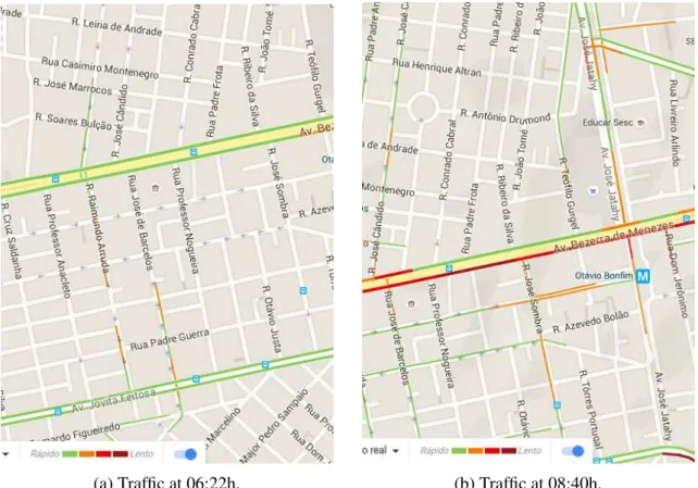
(a) Traffic at 06:22h. (b) Traffic at 08:40h.
Figura 1 – Traffic on the Bezerra de Menezes avenue in Fortaleza, Brazil, at two different times of a day. Source: Google Maps (https://maps.google.com/).
real example of how traffic is influenced by the time of day and, consequently, the time spent to move from one point to another within a large city. It illustrates two different moments of a same avenue in Fortaleza, Brazil. At 19:30h this avenue is completely congested and, thus, the time to cross it is longer than at 20:40h, when the traffic is less intense.
Some recent studies have included the temporal dependence to solve conventional spatial queries, such askNN (DEMIRYUREK et al., 2010c; DEMIRYUREK et al., 2010d; CRUZ et al., 2012) and shortest path (NANNICINI et al., 2012) queries. In time-dependent networks, a kNN query, called TD-kNN, returns thekpoints of interest with minimum travel-time from the query point. As a more concrete example, consider the following scenario. Imagine a tourist in Fortaleza who is interested to visit the touristic attraction closest from him/her. Let us consider two points of interest in the city, the Fortaleza Cathedral and the Iracema Beach. He/she asks a query asking for the touristic attraction whose the path leading up to it is the fastest at that time, the answer depends on the departure time. For example, at 10h it takes 10 minutes to go to the Cathedral (see Figure 2a). It is the nearest attraction. Although, if he/she asks the same query at 22h, in the same spatial point, the nearest attraction is the Iracema Beach (see Figure 2b).
(a) The nearest neighbor at 10h (b) The nearest neighbor at 22h
Figura 2 – An example ofkNN query. The fastest path from the query point to the nearest neighbor is in solid line. The fastest path from the query point to the other point of
interest is in dashed line
segment) and the weight (cost in time) of an edge is a function of the departure time. This way, we can model periodic congestion during rush hour and similar effects, for example.
Processing queries in time-dependent road networks is challenging due to a number of reasons. The space required to store these networks is significantly larger than the space used to store the time-independent ones, since it is necessary to keep, for each edge, the cost to traverse it for every time interval of a day. Furthermore, solutions for conventional queries in static networks can not be directly applied to solve the time-dependent problems. Particularly, it is complicated to apply the well-known speed-up technique of bi-directional search, that starts a search simultaneously from the source and the target, to solve the shortest path problem in a time-dependent network since the arrival time would have to be known in advance for such a procedure.
Figura 3 – An example of taxi call
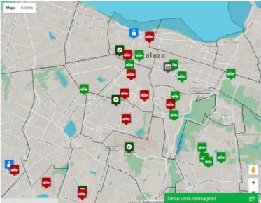
Figure 4 shows a real example of how a cab company may be scattered in a city. This figure illustrates the location of the cabs, of a same company, in Fortaleza city at 10h.
Figura 4 – Arrangement of taxis in the Fortaleza city. Source: (SIMPLES, 2015)
1.2 OBJECTIVES
Given the motivating scenario presented above, the general objective of this work is to study the problem of to find thekpoints of interest (e.g. cabs, ambulances or police cars) which can move to the query point (e.g. a taxi user or a citizen waiting for an emergency service) in the minimum amount of time, proposing efficient and optimal solutions to them. To achieve this objective, we established the following specific objectives:
• To propose a baseline solution, for comparison purposes, to the problem of minimizing the
travel time from points of interest to the query point;
• To propose an efficient algorithm to solve the problem of minimizing the travel time from points of interest to the query point;
• To evaluate the proposed solutions to the problem of minimizing the travel time from points of interest to the query point and to indicate in which types of applications each one should be used;
• To specify and develop a new generator of synthetic networks, varying both the network
size and the density of points of interest;
• To design and develop road networks based in real data about the streets and cabs positions in the Fortaleza city;
1.3 CONTRIBUTIONS
We propose and discuss a solution to this type of query, which is based on the previously proposed incremental network expansion and use theA∗search algorithm equipped with suitable heuristic functions. This solution find thekpoints of interest which can move to the query point in the minimum amount of time. We also discuss the design and correctness of our algorithm and present experimental results that show the efficiency and effectiveness of our solution. We note that, in some cases, the answer returned by a regular TD-kNN query is coincidentally the same as returned by our query, for example, when all the roads allow bi-directional vehicle flow and all conversions are allowed, what is unreasonable in real situations.
The following items summarize the main contributions of this thesis:
• We propose and discuss a baseline solution, for comparison purposes, to the problem of
minimizing the travel time from points of interest to the query point in time-dependent networks. The baseline solution is a variation of the algorithm proposed by Dijstra(DIJKSTRA, 1959);
• We propose an efficient algorithm to solve the problem of minimizing the travel time from points of interest to the query point in time-dependent networks;
• We evaluate the proposed solutions to the problem of minimizing the travel time from
points of interest to the query point in time-dependent networks using synthetic and real data;
• We specify and develop a new generator of synthetic networks, varying both the network size and the density of points of interest;
solutions and a method to access information about adjacency of vertices and history traffic in time-dependent networks.
• Chapter 3 presents the proposed solutions in details;
• Chapter 4 evaluates the proposed approaches; • Chapter 5 discuss the related works;
• Chapter 6 concludes this thesis with a summary of our findings and some suggestions for
2 THEORETICAL FOUNDATION
This chapter describes the concepts and models used to represent time-dependent networks and some of their properties. Section 2.1 shows the definitions of interest point and query point. Section 2.2 presents the graph used to model this network, called time-dependent graph, as well as some concepts necessary to the formulation of the problems investigated in this work. In Section 2.3 we discuss in details the Dijkstra,A∗search (HART et al., 1968) and the Incremental Network Expansion (INE) (PAPADIAS et al., 2003) algorithms, which are of key importance to our proposed solutions. Section 2.4 describes an efficient access method for time-dependent networks. In Section 2.5 we discuss some characteristics of the taxi business. Finally, Section 2.6 concludes this chapter.
2.1 PRELIMINARIES
We start this section discussing some terminologies used in this work. These termi-nologies include interest point and query point.
Definição 1 (Interest Object or Interest Point or Point of Interest - POI) An interest object is any object on a network and it is of interest to users. An interest point is where the interest object is located. We use the terms interest objects and interest points interchangeably. We assume a road network containing a set of interest objects, such as cabs, ambulances, etc.
Definição 2 (Query Object or Query Point) A query object is an object on the network and its influence on interest objects is determined as the query is called. A query point is where the query object is located. We use the terms query object and query point interchangeably.
2.2 TIME-DEPENDENT GRAPH (TDG)
We consider that the structure of a time-dependent road network is modeled by a graph where the vertices represent the intersections of road segments. Those are connected by edges, which the cost to traverse vary with time. More formally, the network is modeled by a time-dependent graph (TDG)G= (V,E,C), whereV is a set of vertices,E is a set of edges
and the cost (time in our domain of interest), represented byC, to traverse an edge is a function of the departure time. In other words, a TDG is a graph in which the costs of the edges varies with time. The concept of TDG is formally defined below.
Definição 3 Atime-dependent graph(TDG) G= (V,E,C)is a graph where: (i) V ={v1, ...,vn} is a set of vertices; (ii) E ={(vi,vj)|vi,vj ∈V,i6= j}is a set of edges; (iii) C={c(vi,vj)(·)| (vi,vj)∈E}, where c(vi,vj) :[0,T]→R
+ is a function which attributes a positive weight for
(vi,vj)depending on a time instant t ∈[0,T]and where T is a domain-dependent time length.
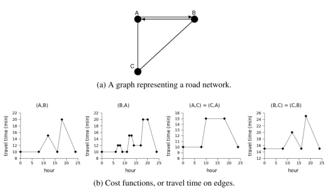
(b) Cost functions, or travel time on edges.
Figura 5 – A graph representing a road network and the costs of its edges for different times of a day.
granularity of 15 minutes during a day. For each edge(u,v), a functionc(u,v)(t)gives the cost of
traversing(u,v)at the departure timet∈[0,T]. We also assume that the travel times of the edges
in the network follow the FIFO property, i.e., an object that starts traversing an edge first has to finish traversing this edge first as well. The general time-dependent shortest path problem in which the departure is immediate, i.e. the user departs exactly at the timet, and in which waiting is disallowed everywhere along the path through the network is NP-hard (ORDA; ROM, 1990a), but it has a polynomial time solution in FIFO networks. Since the travel times satisfy the FIFO property, waiting in a intermediary vertex in a path is not beneficial.
Note that the definition given above does not require the graph to be bidirected. More specifically, the existence of an edge (u,v)does not imply in the existence of the edge (v,u).
Furthermore, there may be opposing edges(u,v)and(v,u)such thatc(u,v)(t)6=c(v,u)(t). As an
example, consider the graph shown in Figure 5 which is a representation of a time-dependent road network. The travel times of its edges for each instant of a day are shown in the graphics in Figure 5b. The pairs of opposite edges(A,C)and (C,A)and(B,C)and(C,B)have the same
cost. However,(A,B)and(B,A), although opposite, have distinct costs.
The time cost to traverse a path from a specific starting time, or departure time, is calledtravel-time. Thetravel-timeis calculated assuming that stops are not allowed because, as discussed before, we consider that the network is FIFO waiting in a vertex do not anticipate the arrival time of a vehicle. Thetravel-timeof a path is calculated considering thearrival timeat each vertex belonging to it. These concepts are formally defined below.
Given that a vehicle starts a path at a vertex of the graph and this path starts at a determined departure time, thearrival-timecalculates the time instant when the vehicle arrives at the other end of the edge. Considering the cost functions shown in 5b, when traversing the road represented by(B,A)at 10:00 am, a vehicle arrives at 10:10 am atA. Note that the operation of
the rest (mod) exists for the calculation of the arrival-time be circular. For instance, consider that one departs fromBtowardsAat t = 24:00,AT(vi,vj,24:00)is 0:10, since the vehicle arrives at
the other end of the edge at this time.
Definição 5 Given a TDG G = (V,E,C), a path p =hvp1, ...,vpkiin G and a departure time t∈ [0, T], thetravel-timeof p is the time-dependent cost to traverse this path, given by T T(p,t) = ∑k−1i=1c(v
pi,vpi+1)(ti)where t1= t and ti+1= AT(vpi, vpi+1, ti).
The above definition shows how the cost of a path, calledtravel-time, is calculated. Given the sequence of vertices that compose a path and the time instant when one starts to traverse this path, thetravel-timeis the sum of the costs to go from one vertex to the next one in the sequence. The cost to go from the first to the second vertex is calculated considering the departure timet. The cost to reach the next vertices depends on thearrival timeat the previous vertex. It is important to notice that this definition does not take into consideration stops at the nodes of the graph, that is, the way to the next vertex in the sequence begins at the same moment when the previous vertex was reached (COSTA et al., 2014). As an example, consider the path
hB,A,Ciin the graph shown in Figure 5a. At a departure timet= 10:00 am, the cost of traversing
this path is given byT T(hB,A,Ci,10:00)which is equal to 25 minutes, since the cost to go from
BtoAat 10 am is 10 minutes and the arrival time atAis 10:10 am and the cost to go fromAto Cat 10:10 am is 15 minutes.
We assume that points of interest as well as origin and destination points are located on a vertex throughout this thesis. On the original network, those points are not necessarily vertices, however, they can be transformed into new vertices of the network as shown in (CRUZ et al., 2012). That work proposes the IncludePOI algorithm which take as input a TDG G and a POI p=h(u,v),τpi, where(u,v)is the edge over which pis positioned andτpis a ratio which
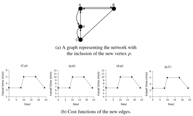
indicates how far pis from the begin of the edge (u). To illustrate how this algorithm works, let us consider that we want to include a new vertex (not necessarily a POI) represented by p=h(C,A),13iin the network shown in Figure 5a. The IncludePOI algorithm works as follows.
It first inserts the new vertex pin the set of verticesV. Figure 6a shows the network with the inclusion of p. As pis a point over(C,A),(C,A)is removed fromE and two new edges(C,p)
and (p,A)are created. The travel time functions for(C,p)and(p,A)arec(C,p)= 13c(C,A)and c(p,A)= 23c(C,A)and the travel time functionc(C,A)is removed fromC. The graphics representing the travel times of the new edges are shown in Figure 6b. Next, as(A,C)is also inE, we need to
repeat the same process executed for the edge(C,A).(A,C)is removed fromEand the edges
is due to Dijkstra (DIJKSTRA, 1959). The algorithm keep, for each verticeu, a labeldistance[u]
with the tentative distance fromsto u. A priority queueQcontains all vertices that describe the current search horizon around s. At each step, the algorithm removes the nodeufromQ with minimum distance froms. So, all outgoing edges(u,v)of u are relaxed, i.e., we check if
d(s,u) +len(u,v)<distance[v]holds. If it holds, a shorter path tovviauhas been found. In
this way,vis either inserted to the priority queue or its priority is decreased. 2.3.2 Incremental Network Expansion (INE)
The problem of processingk-nearest neighbor (k-NN) queries in road networks has been investigated since the pioneering study by (PAPADIAS et al., 2003), where the Incremental Euclidean Restriction (IER) and the Incremental Network Expansion (INE) methods were proposed.
The basic idea of the IER method is to first find the k POIs from the query pointq
(a) A graph representing the network with the inclusion of the new vertex p.
(b) Cost functions of the new edges.
Figura 6 – A new graph representing the inclusion of the vertex pover the edge(A,C)and the
on the Euclidean distance using R-trees (GUTTMAN, 1984). Then, the network distances from qto these POIs are calculated and the distance to the farthest of these POIs is used as an upper bound. Next, all the POIs with an Euclidean distance fromqless or equal to the upper bound are investigated, that is, their network distances are calculated, because they offer a chance to be part of thek-NN result. Figure 7 shows how this method works when one NN is required. IER first retrieves the Euclidean nearest neighbor pE1ofq. Then, the network distancedN(q,pE1)
of pE1is computed. This distance is then used as an upper bound, that is, all the objects closer
(to q) than pE1 in the network, should be within Euclidean distance at mostdN(q,pE1), and,
thus, they should lie in the shaded area of the left figure. Next, as shown in the right figure, the second Euclidean NN, pE2, is found. Similarly, the network distancedN(q,pE2)of pE2 is
computed. Since dN(q,pE2)<dN(q,pE1), pE2 becomes the new NN and the upper bound is
updated accordingly. As the distance to the next Euclidean NN pE3is greater thandN(q,pE2),
the algorithm stops and returns pE2as the nearest neighbor (COSTA et al., 2014).
Figura 7 – Illustration of the Incremental Euclidean Restriction (IER) (PAPADIAS et al., 2003).
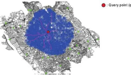
Clearly, the problem with this approach is that, generally,k-NN POIs on the Eucli-dean distance are not alwaysk-NN on the road network distance, especially when time-dependent costs are considered. Thus, several false hits must be investigated. To remedy this problem, the Incremental Network Expansion (INE) algorithm was proposed. It performs network expansion and searches neighbor POIs by visiting vertices in order of their proximity fromq, using Dijks-tra’s algorithm (DIJKSTRA, 1959), until allknearest points of interest are located. Returning to the example shown in Figure 7, as pE2is the NN fromqconsidering the network distance, the
INE algorithm first locates this POI without investigating pE1. The blue shaded area in Figure 8
indicates the search area on the road network of ak-NN query with the INE approach fork= 10 (COSTA et al., 2013). As shown in this figure, the search area is enlarged fromquntil thek POIs have been found.
Figura 8 – Illustration of the Incremental Network Expansion (INE) fork= 10. Source: (HTOO, 2013).
2.3.3 A∗search
TheA∗search is an algorithm that was originally proposed to find the shortest path from an origin to a goal node and it is similar to Dijkstra’s algorithm. The main difference to this algorithm lies in the use of a potential function that guides the search towards the goal. The A* algorithm determines the order in which vertices are expanded in a search by using a cost function, f(v). This function is a sum of two other functions: the known distance from the
starting vertex to the current vertex,d(q,v), plus a heuristic function,h(v), that estimates the
distance from this vertex to the goal.
As A∗ traverses the graph, it follows a path of the lowest expected total cost. It maintains a priority queue of nodes to be traversed and it expands first vertices that appear to be most likely to lead towards the goal. The lower f(v)for a given nodev, the higher its priority. At each step of the algorithm, the node with the lowest f(v)value is removed from the queue. Then, the f and g values of its neighbors are updated accordingly, and these neighbors are added to the queue (CRUZ et al., 2012). The algorithm stops when the destination vertex is removed from the queue or when the queue is empty.
If the potential function h does not overestimate the cost to reach the goal from all v∈V, then A* always finds shortest paths. If h(v) is a good approximation of the cost to reach the goal, A* efficiently drives the search towards the goal, and it explores considerably fewer nodes than Dijkstra’s algorithm. Ifh(v) =0∀v∈V , A* behaves exactly like Dijkstra’s algorithm, i.e., it explores the same vertices.
pass through a number of POIs belonging to certain categories in a given order (COSTA et al., 2013).
2.4 ACCESS METHOD FOR TDGS
Building strategies and algorithms for correct and efficient query processing in time-dependent networks is a challenge, since the common properties of graphs can not be satisfied in the time-dependent case (GEORGE et al., 2007a). Particularly, these networks can not be stored in the same way than a static network, the same applies to the access to the network information. Thus, it emerges the need for storage methods that facilitate the access to the network information and that support the design of efficient algorithms for computing the frequent queries on such networks.
Some characteristics of the time-dependent networks should be considered in the development of this method. First of all, these networks require more space than the static ones to store the costs, since, for each edge, we need to keep the cost to traverse it for each time interval of constant size (COSTA et al., 2014). Another important observation is that the cost of storing the edges of the network grows as the time granularity (number of intervals) increases. Finally, to store the costs of traversing an edge for all the time intervals together implies accessing unnecessary information when retrieving disk page(s) that contains this edge, since the access to the adjacency list is executed to get the cost of the edges for a given time.
Based on these observations, in order to process our queries in a more efficient way, we resort to the access method proposed by (COSTA et al., 2014). It is important to notify that we use this method without any modification or extension. It is composed by three levels, the Time-Level, the Graph-Level and the Data-Level shown in Figure 9. The data pages in the time-level contain pointers to index structures in the graph-level. As a TDG can be seen as a set of static graphs for each time interval, the idea behind the first level is to access first the graph corresponding to a given time interval, avoiding retrieving the edge costs for every possible departure time. The graph-level has an index structure for each time partition, such that it is possible to, given a vertex identifier (Nid), access its adjacency list in the graph corresponding to the departure time. The data pages of the structures in the graph-level contain pointers to a disk page in the data-level that stores the adjacency list of a vertex.
Figura 9 – An access method for time-dependent road networks (CRUZ et al., 2012).
2.5 TAXI BUSINESS
The ground taxicab service is a public transport mode widely used in big cities. Unlike mass public transit (such as buses, trolley buses, trams, subways and ferries), the cabs does not have a regular route and no pre-set schedule. Besides, taxicab is an individual transport service and has higher tariff than mass public. However, taxicab provides a higher quality service.
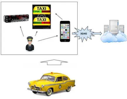
As part of the taxi companies’ efforts on improving their quality of service, in general, each taxi is equipped with a smartphone, which is mainly used to handle taxi bookings and monitor a taxi’s real time status. More specifically, it receives taxi booking tasks from the backend service (taxi call center), and sends back taxi driver’s decision (accept or reject the task) via mobile internet service (3G). Moreover, each smartphone keeps logging and updating a taxi’s real time state by collecting the information from its frontend touch screen. Figure 10 depicts an architecture generally used by cabs companies.
Based on the collected real time information, the smartphone app is able to identify different taxi states. Table 1 lists all the taxi states with their descriptions.
Taxi State Description
FREE Taxi unoccupied and ready for taking a new passenger or booking
POB Passenger on board
STC Taxi soon to clear the current job and ready for new bookings ONCALL Taxi unoccupied, but accepted a new booking
ARRIVED Taxi arrived at the booking pickup location and waiting for the passenger NOSHOW No passenger showing up at he booking pickup location
Tabela 1 – Taxi State
Figura 10 – Architecture generally used by cabs companies.
job:
1. A passenger down a cab with FREE state along a road or a taxi stand.
2. The taxi driver starts the taximeter for a new trip and reports this situation using the smartphone app, which updates the taxi state to POB.
3. During the trip, the taxi state keeps POB while the smartphone app periodically updates the taxi GPS location.
4. The taxi is approaching the destination and the driver presses the FREE button on the smartphone app to update the taxi state to FREE.
A booking job means a cab picks up new passengers, who have made a booking via mobile phone applications (apps), short message service (SMS) or telephone. The typical taxi state transitions on a booking job can be described as next:
driver starts the taximeter.
6. Tthe subsequent taxi state transitions are the same as street job’s procedure, i.e., from street job’s.
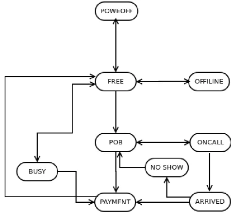
Figure 11 shows a complete taxi state transition diagram, which includes the proce-dures of both street jobs and booking jobs.
Figura 11 – Taxi call state machine.
adopts the event-driven logging mechanism, which are explicitly driven by the taxi state transition events. Therefore, the app captures much more accurate information than the traditional GPS traces, and accordingly provides more opportunities to discover and understand activities of both taxis and passengers.
We use the app log from a large local taxi operator, and select some fields: cabid, latitude, longitude, altitude, accuracy, altitudeaccuracy and timestamp. Table 2 gives the selected fields and a sample record.
cabid latitude longitude altitude accuracy altitudeaccuracy timestamp
982335450 -37316237 -385125479 -6 30 98 Mon Nov 16 2015 11:01:43 GMT-0300 (BRT) 982335450 -37316237 -385125479 -6 30 98 Mon Nov 16 2015 11:01:43 GMT-0300 (BRT) 982335450 -37316654 -38512422 -5 29 100 Mon Nov 16 2015 11:01:44 GMT-0300 (BRT)
Tabela 2 – Selected Fields of Smartphone Log with a Sample (Fonte: (SIMPLES, 2015))
2.6 CONCLUSION
of a time dependent graph where each edge contains a non-negative weights, a linear function according to the time of day. Each edge connects two different nodes of the graph.
We start this chapter stating NN-Reverse-TD Query problem. Next, in Section 3.1, we present a naive solution for this problem, which it will serve as our baseline in our experiments. In Section 3.2, we describe an effective solution for the NN-Reverse-TD query problem.
3.1 PROBLEM STATEMENT
In this section we define the problem of finding the Nearest Neighbor Reverse in Time Dependent Network Query (NN-Reverse-TD Query). In order to formalize this problem we resort to the definitions 3, 4 and 5 presented in Chapter 2.
LetP={p1, ...,pN}be the set of PoIs mapped on vertices of a TDN graphT DG=
(V,E,C). Each PoI p is univocally mapped to a vertice ofT DG. Let a travel time functiontt(s,t),
which computes the travel time from source nodesto target nodet overT DG, wheres,t ∋V. We formalize as N-Reverse-TD query problem as follows:
Definição 6 (NN-Reverse-TD Query Problem) An instance of NN-Reverse Query problem is a tuple NNRQ = (T DG, POI, qp, qt, wt) where T DG is a TDG graph, POI is a set of point of interests where POI ⊆P, qp is a query point such that qp∋V , qt ∈[0, T ] is a non-negative integer representing the query time and mtt ∈ [0, T ] is a non-negative integer defining the maximum waiting time. Given an instance of NNRQ, the problem is to find a p∋P that satisfies the following conditions:
1. tt(p,qp)≤wt
2. ∀ pi∋V |tt(p,qp)≤tt(pi,qp)and p6=pi
Condition 1 stablishes that the travel time should be less than the waiting time wt and condition 2 specifies that travel time from p to qp must be minimal taking into account all POIs.
3.2 NAIVE SOLUTION (BASELINE)
node. Here, the Dijkstra’s algorithm was applied in time-dependent networks.
Dijkstra’s algorithm computes all the shortest path between the source node to every target nodes. Although this solution does not take into consideration the travel time of the each edge, in the expansion of Dijkstra’s algorithm we performed the following criteria:
1. The target is a point of interest, a POI;
2. The non-negative weights is an heuristic functionH(.)adds to each edge an estimate of
the cost to reach any another edge.
The idea is to reach POIs the quickest. Then, after they are reached, we calculate the travel time toquery object, 2. This is our baseline. It is important to stress that our naive solution as well as Dijkstra’s algorithm determine if any two ’shortest path’ only one will be returned.
v0
v1 v2
v3 v4
v5 v6
v7
v9 v8
Figura 12 – Graph of the TDG
(a) Time-dependent edges cost.
input : A query pointq∈V, maximum travel timet∈[0,T] and day timedt
output : The nearest neighbor toqconsidering the maximum travel timet
1 begin
2 poiIds[]←G.getPoiIds();
3 T Tmin←t;
4 POI←-1;
5 VV ←/0;
6 fori = 0 poiIds.size()do
7 Path←Di jkstra(q,poiIds[i],dt);
8 ifPath.getCost()≤tthen
9 ifPath.getCost()≤T Tminthen
10 POI←poiIds[i];
11 T Tmin←Path.getCost();
12 VV←Path.getVerticesVisited();
13 end
14 end
15 end
16 ifPOI>-1then
17 NN(POI,T T min,VV);
18 end
19 end
3.2.2 Query Processing
Algorithm 1 (NN-Reverse-TD-Dijkstra) presents the algorithm to solve the NN-TD Query problem. Using polymorphism,(CARDELLI; WEGNER, 1985), to put the problem in a more abstract structure, we have the input method a query pointq∈V, maximum travel timet ∈
[0,T] and time of daydt.
As the two solutions differs in implementation, the baseline algorithm is similar to the approach Backtracking Search. First, returns allv∈V that representing a point of interest, POI, in graph (line 2). Then, for each point of interest returned, a shortest path check is performed from the point of interest to the query point (line 6 and 7). As previously discussed, this shortest path is an adaptation of Dijkstra’s algorithm, the weight of each edge is replaced by a heuristic functionH(.)that the input value is a time of day and the function returns is time required to
through the edge.
When there is a shortest path from point of interest to query point the next step is to carry out the following checks:
If the total time that was returned in the baseline query is less or equals the input valuet, this ismaximum travel timefor moving frompoint of interesttoquery point(line 8); Second
If the total time that was returned in the baseline query is less or equals a value already attributed (line 3) with the lowest value for moving frompoint of interesttoquery point (line 9);
3.3 NN-REVERSE-TD ALGORITHM
In this section we present the proposed algorithm, show how to perform the pre-processing step. This algorithm is based on the Incremental Network Expansion (INE) algorithm, initially proposed by (??). The INE is an algorithm based on Dijkstra’s algorithm, where initiating a query point, visited all the reachable vertices ofqin order of their proximity, until nearest point of interest are located. However different from previous solutions, our approach does the expansion using a reverse graph,GR, which allows finding and pruning candidates POIs.
The heuristic function of the Naive solution does not take into consideration reverse graph. Its goal is to reach POIs the closer with a shorter time. Then, after these POIs are reached, the better POI is calculated. This solution is not very efficient in the sense that it spends time searching for POIs that are close toq, but that may take a long time to return solution. Clearly, a heuristic that besides considering an estimate to reach POIs can better guide the search for POIs where one can be the service provider, it using the reverse graph heuristic.
Based on this, we propose reverse nearest neighbor solution. The reverse graph was motivated of the heuristicIf you can’t find a solution, try assuming that you have a solution and seeing what you can derive from that ("working backward")from George Pólya’s 1945 book, How to Solve It (POLYA, 1945). This heuristic allows the search to be expanded capture the heuristic functionH(.)not from vertex to destination vertex, but the destination vertex to the
source.
Now we need to formalize the notion of reverse time dependent graph as follows:
Definição 7 (Time-Dependent Graph Reverse (TDG-Reverse)) A reverse graph of G is a graph with the same set of vertices, but the edges are reversed, i.e., if G contains an edge (u,v)then the reverse of G contains an edge(v,u). A Time-Dependent Graph Reverse
(TDG-Reverse) is a graph defined as GR.
Figure 14a shows an example of a time-dependent graphG. Figure 14b illustrates the reverse graphGRofG.
3.3.0.1 Offline Pre-processing
solution we carry out the process to reverse graph,GR, where all directed edges are reversed. 3.3.0.2 Query Processing
As the two solutions differs in implementation, but can have the same input value: query point q∈V, maximum travel timet ∈[0,T] and query time qt. However, the builder objects for handling the query method, the parameter graph is an reverse graph. Algorithm 2 formalizes our solution to the RNN-TD problem.
First, the algorithm loads the reverse graph ofG,GR, from the disk, line 2. Then, the algorithm begins the expansion and inserts qin a priority queueQ(line 9) that stores the set of candidates for expansion in the next step. An entry in queueQis a tuple(vi,AT vi,T T vi),
whereAT vi=AT(q,vi,dt)andT T vi=T T(q,vi,dt). The priority of elements inQis given by
the increasing order ofT T vivalues with the purpose of checking first the vertices that offer a
greater chance to reach thePOIinV.
Next, the vertices are dequeued from Q (line 11). When a vertex u is dequeued fromQit is marked as visited (line 12) in theVisitedlist corresponding to the identifier vertex visited until the current vertex. For example, theVisited[1]list represents that the vertice with identifier (id) equals 1 already been visited. The path from this vertex toqis defined in another list,Parentslist.
For every elementupull of theQcheck if the vertex was added toVisitedlist (line 12), i.e., ifVisitedcontain vertex of theu. Another checking is realized, if maximum travel time t was reached, if this returntrue, an exception thrown path not found for maximum travel time and time of day, line 13 and line 14. And if current vertex is an POI, line 16.
For everyvneighbor ofufor an updatedAT v, we check if it is in theVisitedlist. If this condition is satisfied (which is verified on line 20) "jumps over"one iteration in the loop (line 21), doing this we avoid re-expand vertices unnecessarily. Otherwise, continue checking. T T is updated, added travel time value to reach the current neighbor, line 23. Again to verify that the maximum service time has been exceeded, it has been exceeded, "jumps over"one iteration, line 24. TheParentslist is updated withv, line 27. Already, as the network is expanded,AT viis
The algorithm stops when the vertex isPOIand maximum travel time for service,t, it is not busted, as shown on lines 9 and 10.
Algoritmo 2:NN-Reverso-TD
input : A query pointq∈V, maximum travel timet∈[0,T] and day timedt
output : The nearest neighbor with the minimum route fromPOItoqconsidering the maximum travel timet
1 begin
2 GR←G.reverseGraph();
3 ATq←t+dt;
4 T Tmax←0;
5 Parent←/0;
6 ifq is POIthen
7 ReturnNN(q,0,[q]);
8 end
9 En-queue (q,ATq,T Tmax) inQ;
10 whileQ6=/0do
11 (q,ATq,T Tmax)←De-queueQ;
12 Markqas visited;
13 ifT T current>tthen
14 Return -1;
15 end
16 ifq is POIthen
17 ReturnNN(POI,T T min,Parent)
18 end
19 foru∈ad jacency(q)do
20 ifu is visitedthen
21 continue;
22 end
23 T T current←q.getTravelTime()+u.getTravelTime();
24 ifT T current>tthen
25 continue;
26 end
27 Parent.add(q,u);
28 AT current←q.getArrivalTime()-u.getTravelTime();
29 En-queue (u,AT current,T T current) inQ;
30 end
31 end
As far as we know there is no published research addressing the same query investi-gated in this thesis, which it is: find thekpoints of interest which can move to the query point in the minimum amount of time. Nonetheless, in order to have an idea of how effective our solution is, we compare it to a naive solution used as a baseline. The proposed baseline is a variation of the algorithm proposed by Dijstra(DIJKSTRA, 1959), as discussed previously. With the aim of validate the proposed approach, we have used two different scenarios. In the first scenario, a synthetic data set has been employed. In the second scenario, a real data set was utilized. Besides, both the proposed approach and the baseline were implemented in Java programming language and using the Graphast framework (Group Advanced Research in Database, 2015).
All experiments were conducted on a Intel Core 2 Quad CPU Q6600 server, with 8GB RAM and 2.40GHz, using Ubuntu 11.10 of 64 bits as operating system (see Table 3). We performed the experiments without caching.
Configuration Information
Architecture x86_64(32-bit, 64-bit)
CPU(s) 4
CPU family 6
Processor Intel(R) Core(TM)2 Quad CPU Q6600 @ 2.40GHz
MemTotal 8174664 kB (8GB)
Linux version 3.13.0-65-generic
Distributor ID Ubuntu
Release 14.04 (trusty)
Tabela 3 – Server machine used in the experiments.
We have defined a synthetic cost function, denoted byH(.), where for each edge,
we chose a random speed between 3 km/h and 60 km/h for each interval of the day, so that the time cost given by the ratio between the edge length and this speed satisfies the FIFO property (See Table 4). The cost functionH(.), for a given edgee, has a temporal resolution of 96 points
in time, e. g., a value at every 15 minutes of a day. So, for a certain edgee, the cost in time to traverse emay vary every 15 minutes. FunctionH(.)was inspired by the Haversinemethod
(ABRAMOWITZ; STEGUN, 1964).
Interval of the Day Range to generate speed 1 a.m to 6 a.m 30km/h - 50km/h 6 a.m to 7 a.m 20km/h - 30km/h 7 a.m to 9 a.m 3km/h - 14km/h 9 a.m to 11 a.m 20km/h - 30km/h 11 p.m to 14 p.m 3km/h - 14km/h 14 p.m to 16 p.m 50km/h - 60km/h 16 p.m to 17 p.m 20km/h - 30km/h 17 p.m to 20 p.m 3km/h - 14km/h 20 p.m to 22 p.m 21km/h - 30km/h 22 p.m to 00 p.m 50km/h - 60km/h Tabela 4 – Interval of the day x Speed.
traditionally, there is a low flow of moving objects and the lower speed values are arranged in hours where, generally, there is a high flow of moving objects. Figure 16 shows a graphical representation of the behavior of the cost functionH(.). Figure 16 illustrates the distribution of
the cost functionH(.).
Figura 15 – A graphical representation of the behavior of the cost functionH(.).
4.2 SCENARIO 1: USING A SYNTHETIC DATA SET
Figura 16 – The distribution of the cost functionH(.).
Figure 3 shows the algorithm used in this work to generate time-dependent road networks. This algorithm receives as input parameters: the number of points in the the x-axis (longitude), the number of points in the the y-axis (latitude) and the percentage of vertices that are points of interest. In lines 2 and 3 is calculated the distance between two vertices. Line 7 defines the geographic coordinate in the the x-axis. Line 9 defines the geographic coordinate in the y-axis. Hence, a vertex is created using these two geographical coordinates and added in the graph (lines 11 to 15). After the node insertion, its edges are created, firstly in the vertical direction (y-axis), line 18, and next in the horizontal direction (x-axis), line 19. It is noteworthy that the edges have created two paths and their costs are set according to the Table 4 described previously. It is important to note that this algorithm has a quadratic asymptotic complexity, that is,O(n2).
We evaluated how the proposed approach and the baseline work according to two variables that are shown in Table 5, the network size (i.e., number of vertices) and the density of POIs (i.e., the percentage of POIs in relation to the number of vertices). For each experiment, we vary a parameter and set the other parameter to default values (in bold) and for each triplet of different parameters, we generated 10 distinct time-dependent road networks and executed 10 queries randomly selected for each network, for a total of 100 queries. We calculated upper and lower 95% confidence limits for the relative gain, assuming the data to be normally distributed. As only the network size and the density of POIs affect the cost of the pre-processing of all solutions, we investigate how these costs are influenced by these variables.
Algoritmo 3:Algorithm to generate time-dependent road networks
input : Numberxof latitude points, numberyof latitude points andppercentage of vertices that are POIs
output : The GraphGwithx×yvertices
1 begin
2 interadorX←180÷x;
3 interadorY←180÷y;
4 randomPOI[]←RandomPOI(x,y,p);
5 poi←0;
// iterate to create nodes
6 fori = 0 to xdo
7 longitude←interadorX·i+ (-90);
8 forj = 0 to ydo
9 latitude←interadorY ·j+ (-90);
10 node←Node(latitude,longitude);
11 ifpoi∈randomPOI[]then
12 node.isPoi←true;
13 end
14 G.addNode(node)poi←poi+ 1;
15 end
16 end
// iterate to create edges
17 fori = 0 to (x×y- 1)do
// create parallels edge to the axis abscises
18 ifi < (x×y- x)then
19 edge←Edge(i,i+y);
20 edge.RandomCost();
21 G.addEdge(edge);
22 edge←Edge(i+y,i);
23 edge.RandomCost();
24 G.addEdge(edge);
25 end
// create parallels edge to the axis of the ordinates
26 if(imodx)6=(x-1)then
27 edge←Edge(i,i+1);
28 edge.RandomCost();
29 G.addEdge(edge);
30 edge←Edge(i+1,i);
31 edge.RandomCost();
32 G.addEdge(edge);
33 end
34 end
35 end
Density of POIs 1%, 5%, 10% Network Size 1k, 10k, 100k, 1000k
Tabela 5 – Parameters values of experiments using synthetic data.
4.2.1 Effect of the density of POIs
We set the density of POIs to be 1%, 5% and 10% of the number of points of interest (uniformly distributed). For each density, we generated 10 distinct time-dependent networks with 2000 vertices and executed 10 randomly selected queries withk=1 on each one.
since the number of possible solution grows when the number of POIs increases and the baseline computes all possible solutions.
Figura 17
The effectiveness metric has been used to compare how many times the propose approach has found the optimal solution, that is, the same solution found by the baseline.
Figure 21 illustrates the effectiveness of the proposed approach in time-dependent road networks with 1knodes. Note that, for a POI density of 5% the proposed approach found the optimal solution in 95% of cases. Figure 22 illustrates the effectiveness of the proposed approach in time-dependent road networks with 10knodes. Note that, for a POI density of 5% the proposed approach found the optimal solution in 90% of cases. It is important to note that the proposed approach’s effectiveness decreases as the POI density increases, regardless of the network size.
Figura 18 – Processing Time X POI Density in a 10kroad network.
Figura 19 – Effectiveness in a 1kroad network.
4.2.2 Effect of the network size
In this experiment, we generate 10 time-dependent networks with 1k, 10k, 100kand 1000kvertices. Each one with 10% of points of interest. We executed 10 randomly selected queries withk=1 on each network.
4.3 SCENARIO 2: USING A REAL DATA SET
Figura 20 – Effectiveness in a 1kroad network.
Figura 21 – The average of visited vertices in a 1kroad network.
Figura 22 – The average of visited vertices in a 10kroad network.
Figura 23 – Page about Fortaleza city in Open Street Map Wiki.
4.3.1 Data Sets Pre-processing
In order to build time-dependent road networks, we had to process and extract information from these two data sets. For this, we have used the following strategy:
database. This data set is available as aOSMfile. Then, we used a script called “osm2pgsql” in order to export the information about the road network of Fortaleza to the “ROAD” table.
3. Then, we exported theTaxi Simplesdata set to the “TAXI-CAB” table in thePOSTGIS database. This data set is available as a Comma-separated values(CSV) file, See Ap-pendix A. In this file, the taxi positions follows the GEOLOCATION API specification (GEOLOCATION. . . , 2015) and have an average error of 13.60 meters. This file contains about 1,500,000 records (positions) for 430 cabs. So, there are many registers (points) to the same cab. For this reason, we selected for each cab the register with the highest timestamp. Thus, the “TAXI-CAB” table has only 430 registers, one for each cab. In this step, only the columns “id” and “point_geo” were filled.
4. Finally, we performed the map matching between the taxi positions and the road network, that is necessary to place the cab over a correct street segment. This task was carried out running a geographical query inPOSTGIS, which performs a data interpolation. Figures 25a and 25b show the relationship between the taxi positions and the road network before and after the mapping match process. In this step, the column “gid” in the “TAXI-CAB” table is filled.
(a) Before the map matching process (b) After the map matching process
Figura 25 – The relationship between the taxi positions and the road network
4.3.2 Effect of the density of POIs
4.3.3 Effect of the network size
In this experiment, we generate 100 time-dependent networks with 1k, 10k, 50kand 100kvertices. Each one with 1% of points of interest. We executed 10 randomly selected queries withk=1 on each network. In order to select a snippet of the Fortaleza road network, we have used the following strategy: we choose the square region with the largest number of cabs. The query point was selected randomly, using a strategy proposed by (KNUTH, 1969). The chosen snippets of the Fortaleza road network (with 1k, 10k, 50kand 100kvertices) are illustrated in Figures??.
Figura 26 – Fortaleza road network with 1,000 points.
Figura 27 – Fortaleza road network with 10,000 points.
Figura 28 – Fortaleza road network with 50,000 points.
Figura 29 – Fortaleza road network with 100,000 points.
Figura 30 – Fortaleza road network with 1k, 10k, 50kand 100kvertices (Images obtained using QGIS (QGIS Development Team, 2009)).
It is important to note that two streets may have points in common (corners, for example). In thePostgisdatabase, for a point that belongs to two streets there are two records. However, in the corresponding time-dependent graph, for a point that belongs to two streets there is just one node. For this reason, the number of nodes in a time-dependent graph and the number of corresponding records in thePostgisdatabase are different. Figure 31 illustrates this difference.
Figura 31 – Number of database registers X Number of nodes in the corresponding graph.
network provided byOpen Street Mapis disconnected, the average number of incident edges is very low (close to 1), as illustrated in Figure 32. Figure 33 shows the ratio of executions that found a POI. For example, in the experiment using road networks with size of 1kjust 40% of the executions found a POI.
Figura 33 – Ration of executions that found a POI X Network size.
(a) Network size X Processing time. (b) Network size X Number of expanded vertices.
5 RELATED WORK
In this chapter we review works that relate to our approach and discuss in detail how our solution advances the state of the art. Section 5.1 presents the approaches to find the shortest path in time-dependent networks. In Section 5.2 are discussed the solutions to executekNN queries in road networks. Section 5.3 shows some initiatives to runkNN queries in time-dependent networks. Finally, Section 5.4 discuss two types of proximity queries called Reverse Nearest Neighbor (RNN) and Reverse Farthest Neighbor (RFN) queries.
5.1 TIME-DEPENDENT SHORTEST PATH
This problem has an intrinsically relation with the time-dependent kNN problem, since the nearest POIs from the query depend on the cost (travel time) of the shortest (fastest) path to each POI object. The usual solution to shortest path problem in static graphs is Dijkstra’s algorithm (DIJKSTRA, 1959). In (WAGNER; WILLHALM, 2007), the authors present a survey with many others ideas that have been proposed to find point-to-point shortest paths.
Unfortunately, these ideas would fail when time-dependent networks are considered. Much less work has been proposed to the time-dependent case. The first algorithm that considers a time-dependent variant of shortest paths is addressed in (COOKE; HALSEY, 1966). This algorithm is a modified form of Bellman’s (BELLMAN, 1957) iteration scheme for finding the shortest route between any two vertices in a network.
In 1997 and 1998, Chabini (CHABINI, 1997)(CHABINI, 1998) proposed two types of time-dependent shortest path (TDSP) algorithms in discrete dynamic networks. George and Shekhar proposed (GEORGE et al., 2007b) a time-aggregated graph where they aggregate the travel-times of each edge over the time instants into a time series. Their model has less storage requirements than the time-expanded networks. All these studies assume that the edge weight functions are defined over a finite discrete time window. They proposed two algorithms for shortest path computations. For each time window, the first algorithm computes the shortest path for a given start-time, through the static network. The second algorithm computes the shortest paths which result in the least travel time over the entire time period. Orda et al. (ORDA; ROM, 1990b) proposed a Bellman-Ford based solution where edge weights are piece-wise linear functions.
algorithm, starting from the query objectqall network nodes reachable fromqin every direction are visited in order of their proximity toquntil allknearest data objects are located.
In (KOLAHDOUZAN; SHAHABI, 2004a) the authors presented an approach based on pre-computing the network’s voronoi polygons (NVP) (ERWIG; HAGEN, 2000), indexed by a spatial access method. Using NVPs one can immediately find the first nearest neighbor of a query object and reduce the on-line cost in akNN search. These approaches cannot be directly applied to solve TD-kNN queries. Berchtold et al. (BERCHTOLD et al., 1998) too usedVoronoi diagram, suggest precalculating approximating and indexing the solution space for the nearest neighbor problem inmdimensional spaces. Precalculating the solution space means determining theVoronoi diagramof the data points, cells.
In (HU et al., 2006) the authors developed a network reduction technique where the network topology is simplified by a set of interconnected tree-based structures (SPIE’s). By doing that the number of edges is reduced while all network distances are preserved. They proposed thend (nearest descendant) index on the SPIE such that akNN query on those structures follows a predetermined tree path, avoiding unnecessary network expansion. In (LEE et al., 2009) the authors exploited the search space pruning technique. With the observation that during a search some subspaces of the network with no objects can be skipped, they organized a road network as a hierarchy of interconnected regional sub-networks (Rnets). They speed-up the search performance by incorporating shortcuts that avoid detailed traversal and object lookup within Rnets, allowing bypass those Rnets that do not contain objects of interest.
Kollios et al. (KOLLIOS et al., 1999) propose an elegant solution for answering kNN queries for moving objects in one dimensional space. Their algorithm uses a duality transformation, where the future trajectory of a moving pointx(t) =x0+vxt is transformed into
a point(x0,vx)in a so-called dual space.
Raptopoulou et al. (RAPTOPOULOU et al., 2003) and Tao et al. (TAO et al., 2004) consider the nearest neighbor problem for a query point moving on a line segment, for static or moving interest points. Raptopoulou et al. (RAPTOPOULOU et al., 2003) consider simplified and less effective heuristics for directing and pruning the search in theTPR-tree. Tao et al. (TAO et al., 2004) also consider the general concept of so-called time-parameterized queries.