Thiago Santos Gouvêa
Dissertation presented to obtain the Ph.D degree in Biology/Neuroscience
Instituto de Tecnologia Química e Biológica António Xavier | Universidade Nova de Lisboa
Oeiras,
May, 2016
Striatal dynamics represent
subjective time
A psychophysical study of the neural
Thiago Santos Gouvêa
Dissertation presented to obtain the Ph.D degree in Biology/Neuroscience
Instituto de Tecnologia Química e Biológica António Xavier | Universidade Nova de Lisboa
Oeiras, May, 2016
Research work coordinated by:
Striatal dynamics represent
subjective time
A psychophysical study of the neural
Striatal dynamics
represent subjective time
a psychophysical study of the neural representation of
time by striatal populations
Thiago Santos Gouvêa
A Dissertation presented to the Instituto de Tecnologia Química e Biológica
of the Universidade Nova de Lisboa in Candidacy for the Degree
of Doctor of Philosophy
Joseph J. Paton
que sejas ainda mais vivo
no som do meu estribilho,
tempo,
tempo,
tempo,
tempo
Acknowledgments
This monograph marks the culmination of an unforgettable period.
I am thankful to each of the members of the jury who, by assessing critically the outcome of my work, have honored me with their time and effort. I am thankful in particular to Dean Buonomano and Elliot Ludvig who offer me their fresh perspectives.
I am thankful to my thesis committee, Megan Carey and Christian Machens, who were very generous and helpful whenever besought.
I am thankful to Joe Paton, an outstandingly caring supervisor, and to the Paton Lab, the nest and the family where I seasoned.
I am also thankful to Zach Mainen and the Mainen Lab, for providing the food for thought an eager young PhD student required.
I am thankful to the INDP-2009 class, the partners with whom I took the first steps in this enterprise, and to the larger CNP community for turning a certain indie/synth-pop hit into such a deep mark on me.
I am also thankful to multicultural Lisbon and the Republic of Portugal for having accepted, incorporated, and sponsored me during these formative years.
While often seeking to understand my social environment at the level of collec-tive structures, I ought to express my gratitude to some individuals of outstanding importance[in rough chronological order]: Dr. Dušica Radoš, whose generosity and timely friendship made for a smooth landing; Ali Özgür Argunşah, the Ottoman spirit lifter; Leila Shirai, whose spacious inner universe was a relief to the daily claustrophobia; Joe Paton, who from early on secured his place on this list too; Eric DeWitt, the most generous intellect I’ve ever encountered; Pietro Vertechi, whose sharp intellect is to be handled carefully; and Nadja Oellrich, who brought a new light to this last stretch, bore with me while I wrote this monograph and, most importantly, was there to say the phrase that made all the difference: “When I felt like that, I did notgo sleep.”
Título
Dinâmica estriatal representa o tempo subjetivo — Um estudo psicofísico da representação do tempo por populações neuronais no estriado
Resumo
O tempo é uma das dimensões fundamentais do ambiente. A abilidade de estimar a passagem do tempo é essencial tanto para a aprendizagem como para a performance de comportamento adaptativo em situações naturais. Apesar da importância desta função cognitiva, a forma como esta é implementada no cérebro ainda não é bem compreendida. Estudos mostram que a dinâmica de populações neuronais em diversas áreas cere-brais contém informação sobre a passagem do tempo. Entretanto, não se sabe na maioria dos casos se estes padrões neurais dinâmicos são de fato utilizados na formação dos julgamentos temporais, ou se meramente covariam com a passagem do tempo.
O estriado é uma estrutura dos gânglios da base implicada em várias funções sen-síveis à passagem do tempo tais como aprendizagem associativa, tomada de decisão, e formação de estimativas temporais. Com o objetivo de estudar a representação do tempo por populações neuronais do estriado, nós treinamos ratos em uma tarefa psicofísica de discriminação da duração de intervalos. Enquanto os animais desempenhavam a tarefa, nós monitoramos o comportamento com uma câmera de alta velocidade, assim como a atividade de neurônios individuais no estriado.
Os animais desenvolveram sequências comportamentais altamente consistentes du-rante o intervalo sendo julgado. A variabilidade dessas sequências se mostrou preditiva dos julgamentos comportamentais desde muito antes do momento do julgamento, dando suporte à ideia de que os animais podem estar utilizando padrões comportamentais aprendidos para estimar a duração de intervalos de tempo.
Abstract
Time is a fundamental dimension of the environment. The ability to estimate the passage of time is essential for both learning and performance of adaptive behavior in natural situations. Yet, how this ability is implemented in the brain is poorly under-stood.
Prior studies have shown that population dynamics in a number of brain areas carry information about the passage of time. However, it is not known whether such time-varying activity patterns inform subjects’ judgments of duration or merely covary with elapsing time.
The striatum is an input structure of the basal ganglia implicated in several time-dependent functions such as reinforcement learning, decision making, and interval tim-ing. In order to study the representation of time by striatal neuronal populations, we trained rats in an duration categorization task while continuously monitoring their behavior with a high speed camera, as well as striatal spiking activity.
Animals developed highly reproducible behavioral sequences during the interval be-ing timed. Those sequences were often predictive of perceptual report since early in the trial, providing support to the idea that animals may use learned behavioral patterns to estimate the duration of time intervals.
We also found that the dynamics of neural activity in populations of striatal neurons encode the passage of time, and that the speed with which time-encoding neural activity progressed reflected on the behavioral report of duration judgment. These results could not be explained by ongoing behavior, suggesting that striatal dynamics form an internal “neural population clock” that supports the fundamental ability of animals to judge the passage of time.
Author Contributions
Experiments contained in this monograph were designed by Thiago Gouvêa, Tiago Monteiro and Joseph Paton.
Data were acquired by Thiago Gouvêa, Tiago Monteiro, Joseph Paton, and Filipe Rodrigues.
Data were analyzed by Thiago Gouvêa, Tiago Monteiro, Asma Motiwala, Christian Machens, and Joseph Paton, with contributions of Sofia Soares, Serkan Sülün, João Frazão, and Gonçalo Lopes.
Chapters 2 and 3 largely recapitulate the articles reprinted in appendix A (Gouvêa, Monteiro, Soares, Atallah, & Paton, 2014; Gouvêa et al., 2015a, respectively). These articles were written by Thiago Gouvêa, Tiago Monteiro, Asma Motiwala, and Joseph Paton, with contributions of all authors.
Financial Support
Contents
Acknowledgments . . . ix
Título e Resumo . . . x
Abstract . . . xi
Author Contributions and Financial Support . . . xii
List of Tables . . . xvi
List of Figures . . . xviii
Acronyms xxi 1 Introduction 3 1.1 Biological autonomous machines . . . 3
1.1.1 Sensors and effectors . . . 3
1.1.2 Intelligent behavior is adaptive . . . 6
1.1.3 Temporal structure holds valuable information . . . 7
1.2 Interval timing behavior . . . 7
1.2.1 Interval production . . . 7
1.2.2 Interval reproduction . . . 8
1.2.3 Interval discrimination . . . 8
1.3 Mathematical models of timing behavior . . . 11
1.3.1 Scalar Expectancy Theory . . . 11
1.3.2 Pacemaker-Accumulator models . . . 12
1.3.3 Behavioral-state based models . . . 15
1.3.4 Interval timing as a combination of time-series . . . 16
1.3.5 Coincidence detection over oscillatory processes . . . 16
1.3.6 Time as intrinsic property of network dynamics . . . 17
1.4.1 The basal ganglia . . . 18
1.4.2 Cortices . . . 19
1.4.3 Hippocampus . . . 20
1.5 Our addition . . . 21
2 Structured behavior predicts duration judgments 23 2.1 Introduction . . . 23
2.2 Results . . . 25
2.2.1 Animals learned to categorize time intervals . . . 25
2.2.2 Animals developed temporally structured behavior . . . 27
2.2.3 Ongoing behavior bears information about unfolding perceptual decisions . . . 28
2.2.4 Behavioral trajectory improves choice prediction beyond trial his-tory . . . 31
2.3 Discussion . . . 32
2.4 Materials & Methods . . . 35
2.4.1 Duration categorization task . . . 35
2.4.2 Behavioral set up . . . 36
2.4.3 Video acquisition and tracking . . . 36
2.4.4 Estimating choice probability from ongoing behavior . . . 37
2.4.5 Generalized linear models . . . 38
3 Striatal dynamics represent subjective time 43 3.1 Introduction . . . 44
3.2 Results . . . 44
3.2.1 Striatal neurons show diverse temporal firing patterns . . . 45
3.2.2 Striatal subpopulations show distinct dynamics for different tem-poral judgments . . . 47
3.2.3 Perceptual sensitivity is predicted by neural separability . . . 48
3.2.4 Striatal neural separability is not explained by ongoing behavior 49 3.2.5 Striatum encodes subjective time . . . 51
3.2.6 Intact striatum is necessary for task performance . . . 54
3.3 Discussion . . . 55
3.4.4 Pharmacology . . . 59
3.4.5 Preference index . . . 60
3.4.6 Low dimensional representations of population state . . . 60
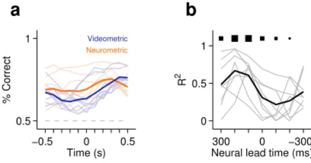
3.4.7 Neurometric curves . . . 60
3.4.8 Videometric curves . . . 61
3.4.9 Time course of classification performance from neural and video data . . . 62
3.4.10 Psychometric curves split by population state at interval offset . 62 3.4.11 Population decoder . . . 63
4 Is the striatal representation of time action specific? 65 4.1 Introduction . . . 65
4.2 A strategy for breaking the one-to-one mapping between categorical judg-ment and action . . . 66
4.3 Variants of the interval categorization task . . . 67
4.3.1 Rule-switching . . . 68
4.3.2 Fixed allocentric rule . . . 72
4.4 Predictions about striatal activity in the task variants given the two standing hypotheses . . . 73
4.4.1 Representation of time per se . . . 74
4.4.2 Time-varying action representation . . . 75
4.5 Methods . . . 76
5 Discussion 79 5.1 Explaining behavior . . . 79
5.1.1 Explaining behavior does not require determining the ’architec-ture of the mind’ . . . 80
5.1.2 Neurophysiology fills the mechanistic gap of behavioral science . 81 5.1.3 On neural representations . . . 83
5.2 A representation of time in the striatum . . . 86
5.2.1 A strengthened hypothesis . . . 87
5.2.2 Origins of striatal dynamics . . . 88
5.3 Two roles for a representation of time in producing behavior . . . 89
5.3.1 Associative learning . . . 89
5.3.2 Time as a feature characterizing the environment . . . 91
A Articles published in peer-reviewed journals 95
A.1 Ongoing behavior predicts perceptual report of interval duration . . . . 95
A.2 Striatal dynamics explain duration judgments . . . 107
B PhD in brief 123
B.1 Annual activities report . . . 123
List of Tables
2.1 Ongoing behavior improves choice prediction beyond allowed by trial history alone . . . 33 2.2 Specification of logistic regression models used to predict choice from
subject identity, interval duration, behavioral trajectory displayed around
List of Figures
1.1 A volley kick . . . 4
2.1 Task schematic and reinforcement contingency. . . 25
2.2 Psychometric functions (mean and standard deviation across sessions and logistic fit). . . 25
2.3 Behavior displayed during stimulus interval is highly reproducible . . . . 26
2.4 Head trajectories are reproducible and idiosyncratic . . . 26
2.5 Pairwise correlations between head trajectories . . . 27
2.6 Distinct behaviors accompany different categorizations of same stimulus. 28
2.7 Head trajectory is predictive of choice . . . 29
2.8 Head trajectory reveals categorization bias. . . 41
3.1 Categorization performance during recording sessions . . . 45
3.2 Example neurons’ raster and peri-stimulus time histogram (PSTH) . . . 45
3.3 PSTH of all neurons in the dataset . . . 46
3.4 Histogram of preference indices . . . 46
3.5 Averaged PSTH of striatal subpopulations . . . 47
3.6 Population state at interval offset allows stimulus categorization — ex-ample session . . . 48
3.7 Slopes of psychometric and neurometric curves correlate . . . 49
3.8 Slopes of neurometric and videometric curves compared to the psycho-metric function . . . 50
3.11 Effect of distance traveled in neural space on decision bias is evident within single subjects . . . 53 3.12 Average speed of smoothly changing population state varies with
percep-tual report . . . 54 3.13 Time decoded from striatal activity at different time points within
stim-ulus period . . . 55
3.14 Time decoded from striatal activity during entire stimulus period . . . . 55
3.15 Duration judgments are impaired following muscimol inactivation of the striatum . . . 56
3.16 (A) Movable microwire bundle array (Innovative Neurophysiology) used
for all neural recordings. (B) Histogram of firing rates for all selected cells (bin size 1 spike/s). (C) Schematic representation of the striatal record-ing sites. Coronal slices at intermediate anterior-posterior (AP) positions are show for reference (left to right, rats Bertrand, Edgar and Fernando). Colored rectangles show the approximate dorsal-ventral (DV) position of the wire bundles across recording sessions and horizontal black lines represent session-by-session recording sites, for 10, 9 and 18 recording sessions, respectively. . . 57 3.17 (A) Histology slices and schematic representation of the location of saline
and muscimol injections. Coronal slices at intermediate AP positions are shown for reference at +0.84mm(left, rat Albert), +1.68mm(center, rat
Yuri) and +0.60mm(right, rat Zack) from Bregma. Vertical grey bars
represent the location of the cannula placements. Yellow asterisks show
the approximate DV position from where the injectors extended 1.5mm
bellow the cannulae. . . 58
4.1 Contingency of an interval categorization task that breaks the one-to-one
mapping between categorical judgment and action . . . 66
4.2 Illustration of behavioral box used both in the original task and in the
rule-switching version . . . 67
4.3 Example session of rat performing the standard interval categorization task . . . 67
4.4 Example session of a rat performing under theleft-shortcontingency . . 69
4.5 Performance over consecutive sessions with alternating contingencies . . 70
4.7 Performance deteriorates in the rule-switching task under multiple diffi-culty levels . . . 71 4.8 Illustration of behavioral box used in the task with a fixed allocentric rule 72
4.9 Example session of a rat performing in the second task variant . . . 73
4.10 Scheme of a network that performs two distinct interval categorization
tasks with the same dynamics . . . 74
4.11 Stimulus form and output of the network from figure 4.10 . . . 74
4.12 Scheme of a network that performs two distinct interval categorization
tasks with fixed activity-output mapping . . . 76
Acronyms
2AFC two alternatives forced-choice. 9, 10
AI Artificial Intelligence. 83–85
AIC Akaike information criterion. 32
ANN Artificial Neural Network. 84
AP anterior-posterior. xix, 57–59
auROC area under the ROC curve. 46
BeT Behavioral Theory of Timing. 15, 21
BIC Bayesian information criterion. 32, 33, 38, 63
CSC Complete Serial Compound. 90
DV dorsal-ventral. xix, 57–59
EAB Experimental Analysis of Behavior. 80–83, 89
FI Fixed Interval. 7, 8, 19
ISI inter-stimulus interval. 90
ITI inter-trial interval. 90
LDA linear discriminant analysis. 30, 37, 41, 48, 60, 61
LeT Learning to Time. 15, 16, 21
MTS Multiple Time Scale. 16
PCA principal component analysis. 38, 59
PFC prefrontal cortex. 17, 19
PI Peak-Interval. 8
PSE point of subjective equivalence. 9, 10
PSTH peri-stimulus time histogram. xviii, 45–47, 59
RNN Recurrent Neural Networks. 17–20
ROC receiver operating characteristic. 29, 37, 46, 60
SET Scalar Expectancy Theory. 11, 12
STM Spectral Timing Model. 16
Chapter 1
Introduction
1.1
Biological autonomous machines
Intelligent behavior, as displayed by a variety of biological species, emerges from the organization of biological matter. What is special about that form of organization? An answer to this question should describe how do cells, the fundamental units composing biological agents, compose devices able to convert different forms of energy emanating from the environment into usable signals, and how those signals combine to generate appropriate behavioral responses.
1.1.1
Sensors and effectors
A fair amount is known about how animal cells can function as sensors (e.g., pho-toreceptor cells in the retina, hair cells in the cochlea) or motor effectors (e.g., muscle fibers). Perhaps less satisfactory though still extensive is our understanding about how do physiological signals originated in the sensory periphery organize to give rise to representational systems in the brain. Knowledge currently available in any standard neuroscience textbook (e.g., Kandel, Schwartz, & Jessell, 2000) allows descriptions such as what follows:
Stunt I
the ball approaches, crossed from the corner arc, photons flying off a light source — either the sun or artificial floodlights — hit the ball and bounce back toward the player’s eyes. Beams of photons, focused on his retina by his eyes’ lenses, are absorbed by opsin proteins sitting on the membrane of photoreceptor cells that compose the light-sensitive epithelium in the back of his eyes. The absorption of photons by pigment molecules nested inside opsin proteins induces conformational changes that lead to the activation of enzymes that modify the cytoplasmic levels of second-messenger molecules, beginning a signaling cascade. Elements of the signaling cascade alter the conductance of the photoreceptor cells’ membrane, generating electric sig-nals that propagate to the axon termisig-nals where they modulate neurotrans-mitter release at synaptic contacts with other cells composing a feedforward network that ultimately conveys the signal to the brain in a topologically
organized manner (as if throughlabeled lines).
At this stage, electromagnetic energy from the environment has been detected by the biological machinery composing his eyes, and the signal has been conveyed to his central nervous system. On its path through different processing stages in the brain, the signal reaches the primary visual cortex in an organized manner — that is to say that different features of the visual scene induce predictable activity patterns in his cortex, thus constituting a
neuralrepresentationof the visual world.
The visual scene happens to be a soccer ball flying over the goal area where an opponent defender deflects it toward our striker. He fixates his gaze on the approaching ball while the goal shows in the periphery of his field of view — as reflected by the neural representation in his visual cortex. Electric signals propagate from there: information flows across the brain, ultimately influencing endogenous neural dynamics in some other brain system from where motor commands are issued. The signal now travels down the axons on his spinal chord via multiple parallel paths targeting different muscle groups. After reaching motor neurons in the ventral horn of the spinal chord, the signal leaves the central nervous system to reach the muscles where acetylcholine release modulates cytosolic levels of calcium inside muscle fibers thus changing the conformation of structural proteins, contracting and relaxing muscles and repositioning bones relative to each other. From the perspective of the camera, the player is adjusting his posture and unleashing the volley in the precise moment the ball comes to reach, his instep hitting the center of the ball in a firm and precise kick. His brain has successfully routed the signals captured by his retina to his musculoskeletal system so as to score that goal.
Stunt II
On another green patch not distant from there, a hungry bird sits on a tree branch. Landing on it was an effortlessly acrobatic move. He has been sitting there poking at the tree holes for many seconds already. It is probably the first time he comes to this particular tree, but he has generally had good luck with trees of such dense foliage in the past. There is a large number of dried fruits, which is not an encouraging sign in itself, but he still expects insects to be relatively abundant here. In fact, given how long he has been exploring this tree, he should expect to have caught some bugs by now. He trusts his senses: up to that point, no prey was there to be detected. At least a full minute has passed. Is it time to acknowledge a minor defeat, spread the wings, and change his bet? Or would that be an impatient and deleterious move?
branches. However, in order to make this decision he can’t rely solely on stimuli that are presently available to his senses. Instead, he needs to take into account estimates of variables such as the probability of capturing preys per unit time spent on a given tree.
The neural representations and computations supporting this temporal decision could not be found in the reference textbook.
1.1.2
Intelligent behavior is adaptive
Finely sensing the environment and performing dexterous motion acts are indeed re-markable achievements of some biological forms. These abilities, however, do not suffice to explain the appearance of intelligence conveyed by their behavior. Instead, it is the appropriateness of behavior to different situations that compels the observer to infer in-telligence — had the striker invested his dexterity into scoring an own go, fans wouldn’t deem him as much respect. In fact, intentionally emitting unfit behaviors is at the heart of certain types of humor, supposedly for violating expectations about intelligence. Sim-ilarly, the bird must deploy its flying apparatus at the appropriate occasions. Beyond producing actions that are biomechanically fit, agents need to be able to identify what behaviors are appropriate, and when to emit them.
1.1.3
Temporal structure holds valuable information
In order to decide what behaviors to emit on a given context, a subject ought to I) characterize the context, and II) estimate the consequences of the different behaviors in its repertoire. Time plays a double role in this process. On the one hand, it is one of the features defining context; on the other hand, it forms a dimension along which events organize in ways that allow the inference of causal links between behavioral responses and their consequences. This topic is expanded in chapter 5 (see section 5.3 on page 89).
1.2
Interval timing behavior
Behavior is sensitive to temporal regularities in the environment. Temporal features of the environment across different time scales are of behavioral importance. The rel-evance of timing can be seen, for example, on the dynamics of sensory events (e.g., speech recognition requires fine discrimination of subsecond fluctuations in sound), the dynamics of motor behavior (as in complex movements composed of a well timed se-quence of simpler actions), and in the way behaviors are distributed over larger time scales (e.g., foraging behavior).
Behaviors relying on estimation of time in the range of seconds are collectively known asinterval timing, and a number of behavioral paradigms have been employed to study it. While interval timing paradigms have been summarized elsewhere (Grondin, 2010; Merchant & de Lafuente, 2014), a non-exhaustive list containing some popular ones is presented next:
1.2.1
Interval production
Interval production tasks are those in which the behavioral correlate of the subjective estimate of interval duration consists of the timing of a self paced, observable response, relative to the occurrence of a reference event (e.g., the last reward). These tasks are referred to asprospective timing tasks.
Under this contingency, animals show temporal discrimination — i.e., they tend to emit the behavioral response preferentially during a specific time window that ends with delivery of the reinforcer, even in the absence of any external contextual cues signaling the occasion. Specifically, animals tend to display a low rate of responding during the beginning of the FI, and change abruptly to a high response rate at around two-thirds of
the interval — it is the so calledbreak-and-runpattern (Cumming & Schoenfeld, 1958;
Schneider, 1969). The breakpoint at which response rate increases is taken to indicate the animal’s estimate of proximity to the end of the FI.
In a variant known as the Peak-Interval (PI) procedure, the reinforcer is omitted in a small fraction of trials, so that a second breakpoint occurs in which responding returns to a low rate (Meck & Buhushi, 2010).
These tasks are attractive due to the simplicity of the contingencies employed. How-ever, animals performing them do not have a strong incentive to be precise — by re-sponding at times distant from the reinforced occasion, subjects incur no cost other than that of executing the response itself, which is supposedly low compared to the cost of missing an available reward. As a consequence, the link between time estimation ability and observable behavior is weakened.
1.2.2
Interval reproduction
Interval reproduction tasks combine the prospective component of production tasks
with aretrospectivecomponent: the timing of the behavioral response to be produced
by the subject must match the duration of an interval presented by the experimenter (e.g., Treisman, 1963; Michon, 1967; Wing & Kristofferson, 1973; Pastor, Artieda, Jahanshahi, & Obeso, 1992; Jazayeri & Shadlen, 2010, 2015).
This type of task has the advantage over production tasks that intervals of different duration can be elicited flexibly across trials. Perhaps due to the cognitive flexibility demanded, these tasks most commonly employ primates as subjects. One downside of these tasks is the difficulty in teasing apart behavioral variability between the retro-spective and proretro-spective components — i.e., variability in estimating/remembering the reference interval, as opposed to variability in producing the desired interval.
discriminate between contexts when the probability of emitting a given behavioral re-sponse is different for different contexts, as shaped by its context-specific reinforcement
history. In this case, contextual stimuli are said toset the occasionfor that behavioral
response, and behavior is said to be under stimulus control (Skinner, 1965; Catania, 1999).
In interval discrimination tasks, the contextual trait setting the occasion for different
behaviors istime— i.e., the duration of a stimulus interval that has been presented to
the subject prior to the behavioral response. Usually, these tasks are set to reinforce two distinct behavioral responses differentially and non-probabilistically (e.g., Stubbs, 1968; Platt & Davis, 1983; Leon & Shadlen, 2003; Balcı et al., 2008; Gouvêa et al., 2014), and are therefore described as binary-choice, or two alternatives forced-choice (2AFC) tasks. That is the case for all tasks presented in this section.
Interval discrimination tasks are purely retrospective timing tasks in the sense that, unlike in prospective timing tasks, the timing of the emitted behavior is irrelevant — with the trivial exception that some deadline for responding is often imposed. Instead, a given behavioral response will or will not be reinforced contingent solely on the duration of the interval that preceded it.
Temporal bisection
In temporal bisection tasks (Stubbs, 1976; Church & Deluty, 1977; Platt & Davis, 1983; Maricq & Church, 1983), two distinct stimulus intervals — one short and one long — set the occasions in which either of the two behavioral responses is reinforced (i.e., choosing to emit one of the responses is reinforced following presentation of the short stimulus, while the alternative choice is reinforced following presentation of the long stimulus). Importantly, subjects are not allowed to respond before stimulus termination. The behavioral correlate of interval estimation is the choice probability conditional on stim-ulus, and generally subjects will choose the reinforced option in a nearly deterministic manner.
The unconstrained contingencies for intermediate stimuli do not incentivize subjects to discriminate time to the best of their ability, and therefore are not well suited for study of the precision of temporal perceptual abilities. Instead, the interest elicited by temporal bisection tasks comes from observing where do subjects place their PSE spontaneously, or how is that affected by neurobiological manipulations (e.g., Maricq & Church, 1983). A phenomenon of particular interest is the regularity of the behavior that emerges spontaneously under such unconstrained contingencies — the fact that the PSE is reproducibly well approximated by the geometric mean of the reinforced stimuli is often taken as evidence that subjective time evolves in a relative scale, in agreement with the scalar-timing hypothesis (Gibbon, 1977).
Switching task
The switching task is a simplified variant of the bisection task in which only extreme, reinforced stimuli are presented, and animals are allowed to respond during the stimulus period instead of being forced to wait for stimulus completion (Balcı et al., 2008). In this case, the behavioral correlate of interval estimation is the time at which the subject switches away from the short response given presentation of a long stimulus. One advantage of the switching task over the bisection and categorization tasks is that it allows a read out of the PSE as a continuous variable on single trials.
Interval categorization
Because in this paradigm every stimulus presentation sets the occasion for discrimi-nation, animals are incentivized to utilize sensory information to the best of their ability, and failure in emitting the reinforced response is taken to indicate that the subject is operating in the vicinity of its perceptual limits.
Within the interval timing literature, interval categorization tasks have been employed with different model organisms such as pigeons (Stubbs, 1968), human-(Creelman, 1962), and non-human primates (Leon & Shadlen, 2003). In the current monograph, this paradigm is employed to study the neural representation of temporal judgments in the rodent striatum. A description of the task can be found in section 2.4.1 of this volume, as well as in Gouvêa et al. (2014). Additionally, two new variants of this task are introduced in chapter 4.
1.3
Mathematical models of timing behavior
The array of behavioral paradigms listed above generates a large amount of data on interval timing behavior. A number of mathematical models exist that attempt to quantitatively capture it, some of which are listed below:
1.3.1
Scalar Expectancy Theory
As noted by Gibbon (1977), a very conspicuous regularity found across a large number of studies is that the variability of time estimates, as measured by the standard deviation, scales linearly with the mean duration of the estimated interval across a large range of interval durations. In other words, the coefficient of variation ( = standard deviation /
mean ) is constant across a range of durations. This phenomenon is known as thescalar
property of interval timing, and constitutes the cornerstone of his Scalar Expectancy Theory (SET).
In that same work, Gibbon proposed that interval timing behavior comes about by acomparisonmechanism based on theratiobetween the inverse of the estimated time until reinforcement ("an instantaneous rate-of-reinforcement estimate", Gibbon, 1977, p. 281), and the baseline rate of reinforcement estimated over an entire session.
Of crucial importance in this proposition is the role played by the manner by which the time until reinforcement is estimated. While refraining from proposing any mecha-nistic or otherwise structural hypothesis about how time estimates are produced (SET is "a theory properly described as a discrimination theory of temporal control", Gibbon,
under different reference intervalsT — elicitation (xidentically distributed irrespective
ofT), absolute timing (xdistribution is centered onT and has a fixed shape), Poisson
timing (xis Poisson distributed with mean and variance T), and scalar timing (x is
normally distributed with meanT, and standard deviationγT whereγis the constant
coefficient of variation). As can be noted already from their descriptions, only the latter generative model is consistent with the scalar property.
Once scalar timing has been established as the only reasonable form of generating estimates of time until reinforcement, the "expectancy ratio comparator" decision mech-anism is then shown to fit well different behavioral paradigms. Behavior under temporal production contingencies are postulated to be generated by undergoing a break-and-run transition whenever the ratio between instantaneous and baseline reinforcement rates
(a.k.a. expectancies) cross a threshold that is arbitrary but fixed. Interval
categoriza-tion, on the other hand, is implemented by comparing the ratio between the expectancies estimated assuming the stimulus belongs to either of the two categories.
While scalar timing coupled with expectancy based decision making mechanims can describe a wide range of behavioral results, an attempt to link SET to an algorithmic implementation of interval timing behavior was only made later, when Gibbon proposed what he calls an information processing model of interval timing (first introduced in Gibbon & Church, 1984). This model is introduced below.
1.3.2
Pacemaker-Accumulator models
Pacemaker-accumulator models are perhaps the most widely used models to explain behavioral data on a number of paradigms in the interval timing field. Their origins, however, point to a different class of temporally structured biological phenomena.
As noted by Crozier and Stier (1925) for a number of rhythmic neuromuscular phenomena in arthropods, frequency increases monotonically with temperature — from the velocity of progression in ants to the frequency of chirping in crickets, abdominal respiratory movements in dragonfly larvae, and even flashing in fireflies. Taking the known relation between rate of chemical reactions and temperature to a surprising
limit, the authors apply the Arrhenius equation1 to fit the rhythmic neuromuscular
arthropod behaviors.
They found a surprising level of similarity in the single free parameter of the model,
catalyst (Rice, 1923 apud Crozier & Stier, 1925). On this regard, Crozier and Stier (1925, p. 429) put forth the following observation:
The surprising degree of quantitative concordance evident in this list led to the assumption that not only do such rhythmic activities reflect the deter-mination of the frequency of neuromuscular movements through the agency
of chemical transformations, but that thegoverningchemical process must
be of identical type in the several instances — at least in the sense that there is involved a common catalyst. The conclusion is the more permissible because the activities compared may be taken to involve "central nervous discharge" as controlling element, and are thus truly homologous.
The idea that the rate of discharge of processes taking place in the central nervous system controls the speed of temporally structured behavior extends from that day to the present. Whether temperature can be a significant determining factor in modulating interval timing, however, was yet to be tested. Hoagland took that step after the following reasoning (Hoagland, 1933, p. 268):
If our judgments of time depend upon an underlying chemical "master re-action," in, let us say, cells of the brain, modification of the internal body temperature might be expected to alter judgments of time intervals in a way consistent with the Arrhenius equation and might yield a significant temperature characteristic. Such a finding might even imply a specifically catalyzed, irreversible chemical mechanism controlling the consciousness of duration.
Using as subjects his feverish, influenza-infected wife and a student who "agreed to
submit himself to diathermy treatment"2 (Hoagland, 1933, p. 270), Hoagland found
that the relation between body temperature and behavior in an interval production task are well fit by the Arrhenius equation, albeit with higher cross-subject variability in temperature characteristic.
Taking Hoagland’s suggestion that subjective time might arise from a rhythm gen-erating "chemical clock" that is susceptible to global variables such as temperature, Treisman (1963) proposed an algorithmic model "devised in an attempt to explain and relate the psychophysical findings" (p. 18) of a series of interval timing experiments presented in the same article. In his own words (Treisman, 1963, p.19):
Hoagland (1933) compared his "chemical clock" to pacemaker neurons. These produce impulses at rates which may vary and transmit them along axons whose speeds of conduction are relatively fixed. Analogous assump-tions are made here, but no hypotheses about the neural identity of the components of the model are intended
Treisman’s model is composed of a pulse generator (pacemaker), a counter, a storage (memory) mechanism, and a comparator (decision mechanism). Additionally, an arousal center controls the pace of pulses. The pulse generator has a basic interpulse interval
with mean t0 and standard deviationσt. Pulses are emitted with a mean interpulse
intervalt′ defined as
t′=t0q (1.1)
, whereqis the arousal level. During an interval to be estimated, the counter keeps track of the number of pulses emitted. The pulse count can be transferred to the storage, or it can be compared to a stored value to produce a decision (e.g., increase the rate of responding in an interval production task). Additionally, several noise terms are introduced at different stages of the process.
The impact of the different noise terms on variability in behavioral output is the focus of the article in which Gibbon and Church (1984) introduce their information processing model of interval timing. Briefly, the authors show that, in order for the output of the pacemaker-accumulator model to display the scalar property, variability needs to be postulated at the level of two variables that get multiplied — within trial-interpulse intervals and cross-trial pulse rate (t0 and q in equation 1.1, respectively). In the absence of slow, cross-trial noise, variance increases with the square of the mean of the estimated interval, implying that the coefficient of variation is gets smaller for longer intervals — in other words, estimates of longer intervals should be relatively more precise than that of short ones, in conflict with empirical knowledge (Gibbon, 1977).
internal clock were proposed by both Hoagland and Treisman — respectively temper-ature and arousal, although to what extent the latter can be independently verified is arguable.
1.3.3
Behavioral-state based models
Under environments with strong temporal regularities, animal behavior is known to become temporally structured (e.g., Skinner, 1948; Hodos, Ross, & Brady, 1962; An-derson & Shettleworth, 1977; Haight & Killeen, 1991; Machado & Keen, 2003; Balcı et al., 2008; Ölveczky, 2011). Stemming from this observation, some authors have posited that animals might estimate the passage of time directly from transitioning through a series of behavioral states — the data presented in chapter 2 of this monograph speaks to this idea.
Behavioral Theory of Timing
Observing that under interval timing tasks animals tend to display reproducible se-quences of interim behaviors, Killeen and Fetterman (1988) noted that these behaviors could themselves serve as discriminative stimuli. The authors then propose a simple model, known as Behavioral Theory of Timing (BeT), in which each interim behavior is associated with a different state. The transition between states is postulated to be triggered by the emission of a pulse from a Poisson pulse emitter. The rate of the pulse emitter is controlled by the rate of reinforcement, the fluctuation of which introduces the multiplicative variance that guarantees the scalar property — making BeT formally very similar to the pacemaker-accumulator models of Treisman (1963) and Gibbon and Church (1984).
Learning to Time
The learned variable in LeT is, effectively, a linear readout vector, and the equa-tions governing readout learning are reminiscent of methods applied to artificial neural networks — namely, minimization by gradient descent of a convex error function such as the sum of squared errors.
1.3.4
Interval timing as a combination of time-series
The idea of estimating the duration of an interval by combining (e.g., linearly summing) a number of different time-varying processes is shared between LeT and several other
models, some of which preceded it. This idea is akin to the mathematical notion ofbasis
functions: a new function (e.g., the degree of belief that a given time point matches true current time, as a function of a range of time points) can be expressed as a sum of pre-existing functions. Alternatively, the different time series can be interpreted as forming a feature space well suited to represent/approximate arbitrary temporal patterns.
These models differ on how the time-varying processes (or basis functions) are gen-erated. In the Multiple Time Scale (MTS) model proposed by Staddon and Higa (1999) the basis functions are monotonically decreasing functions that, after being triggered by an input stimulus, decay at different rates. Similarly, the basis time-series in the Spectral Timing Model (STM) of Grossberg and Schmajuk (1989) are produced by pro-viding a range of time scales, but their form and nature differ: they are not functions, but the time evolution of a set of dynamic variables governed by coupled differential equations that result in a set of progressively widening unimodal patterns. Time se-ries of similar shape are proposed by Ludvig, Sutton, and Kehoe (2008), though in this work the time series are defined by functions describing the occupancy of linearly spaced temporal receptive fields by an exponentially decaying trace. In the model presented by Shankar and Howard (2012), the time series are generated by leaky integrators with different leak rates that effectively perform a Laplace transform of the stimulus history; importantly, the transformation can be (approximately) inverted by a linear read out unit.
1.3.5
Coincidence detection over oscillatory processes
milliseconds. Any system that needs to generate reliable dynamics on a time scale much longer than that of its components, as is the case in the brain, is faced with a difficult problem. Miall (1989) noted that a solution could lie in the combinatorics of oscillatory processes: if a number of sine wave oscillators with slightly different periods are triggered in phase synchrony, the time it will take until the initial phases synchronize again is much longer than the period of the average oscillator3. Miall proposes that real neurons in the brain could implement a clock with time scales much longer than that of single neurons if neurons could function as oscillators. Bearing on the literature on the neurobiology of timing, Matell and Meck (2004) proposed that the oscillatory processes could be implemented by neurons in the cortex, while the oscillation detectors could lie in the striatum.
1.3.6
Time as intrinsic property of network dynamics
On a largely parallel historical thread, artificial neural networks have been explored as useful computational architectures loosely inspired in biological brains. For a long time the field was dominated by feed-forward architectures (Palnitkar & Cannady, 2004),
perhaps due to the success of theperceptron (Rosenblatt, 1958) as both a cognitive
the-ory of discrimination and a classification tool with applications in artificial intelligence. In these types of network, neurons are organized in layers, and connections are estab-lished exclusively unidirectionally between neurons in adjacent layers. This results in a process in which time is not a relevant dimension, as the computation of interest (e.g., the categorization of a static input pattern) is often performed on a single feed-forward sweep through the network.
An alternative architecture of interest is that of Recurrent Neural Networks (RNN). Unlike feedforward networks, in RNN any neuron can be connected to any other. As a result, activity reverberates giving rise to interesting dynamics that are in closer resemblance with neurobiological patterns. RNNs displaying attractor dynamics have
been proposed to implement thepersistent activitypattern thought to be used by neural
circuits in the prefrontal cortex (PFC) to implement working memory (Wang, 2001). While useful to store the memory of a static input for an extended period of time after termination of stimulus presentation, persistent activity patterns lack the dynamics necessary to encode information about the passage of time.
Maass, Natschläger, and Markram (2002) proposed that a RNN could also be used to encode the memory of a stimulus in a dynamic way so that both stimulus identity and
timing could be inferred. As in attractor networks, memory of stimuli persists in RNNs displaying dynamic trajectories for a period longer than the time constant governing the dynamics of individual neurons. In line with this observation, it has been noted that the dynamics of RNNs could also be used to solve the interval timing problem (Buonomano & Merzenich, 1995; Buonomano & Maass, 2009; Buonomano, 2014; Goel & Buonomano, 2014). On this regard, the activity of single neurons composing a RNN can be seen as separate time series that can be combined to represent/approximate arbitrary temporal patterns, as in the models introduced in section 1.3.4.
Recent work showing RNNs can be trained to support temporal warping (Goudar & Buonomano, 2015) suggests a phenomenon analogous to multiplicative variance, re-sponsible for the scalar property in pacemaker-accumulator models, might emerge from RNN dynamics.
1.4
Encoding time with neurons: a brief review
A representation of time can be implemented by artificial neural networks such as RNNs. But how is the passage of time represented in the activity of biological brains? Insights into the neurobiology of interval timing is provided by a number of studies ranging from lesion and pharmacology to direct observation of neural activity under temporally regular contingencies. Potentially time-encoding neural activity has been observed across a number of brain areas — although evidence of their use in informing behavior is often missing. A number of these studies addressing the question of how does the animal nervous system keep track of time are presented next.
1.4.1
The basal ganglia
The dopaminergic system Patients of Parkinson Disease underestimate time
on the speed of subjective time estimation (e.g., Maricq & Church, 1983; Balcı et al., 2008).
Selectively lesioning dopaminergic cells in ventral midbrain abolished completely the temporal structure in rate of responding in an interval production task (Meck, 2006). The effect could be reproduced by lesioning only the cell terminals in striatum, suggesting the effects of dopaminergic manipulations on interval timing are mediated by computations taking place in the striatum.
Striatum Striatal activation has been reported in humans performing interval timing
task (Hinton & Meck, 2004; Harrington, Zimbelman, Hinton, & Rao, 2009), thought the content of striatal activity cannot be inferred from these studies.
Spiking activity recorded in the striatum of monkeys performing tasks containing a delay period of fixed duration revealed groups of neurons becoming active at different points in time realtive to delay onset, thus allowing experimenters to decode time from neural activity (Jin, Fujii, & Graybiel, 2009; Adler et al., 2012), In both these studies, however, activity was recorded during performance of tasks for which time estimation was irrelevant given the reinforcement contingencies. Therefore, whether the observed neural dynamics constitute a representation of time used to guide behavior or they merely covary with the passage of time cannot be assessed.
A comparable pattern of activity was found in the rodent striatum (Mello et al., 2015) during an interval production task. This study presents the advantage of having being recorded under contingencies for which time matters — animals were trained to lever press under FI reinforcement schedules, the duration of the interval varying over blocks of tens of trials. Interestingly, the authors found that the time window tiled by the firing of striatal neurons re-scaled to match the duration of the FI, and that, during block transitions, the number of trials needed for behavior to adjust was matched by the time course of neural adaptation, suggesting this neural code for time might be used to inform behavior.
1.4.2
Cortices
Prefrontal cortex During performance of working memory tasks, the PFC is
& Jung, 2009), and time encoding neural activity have been observed both in primates (Machens, Romo, & Brody, 2010) and rodents (Kim, Ghim, Lee, & Jung, 2013; Xu, Zhang, Dan, & Poo, 2014).
Parietal cortex The parietal cortex has been implicated in functions such as
cat-egory representation (Freedman & Assad, 2006), working memory (Harvey, Coen, & Tank, 2012), and accumulation of sensory evidence (Shadlen & Newsome, 1996, 2001; Hanks et al., 2015).
In the working memory task, the parietal cortex has been shown to display sequential activity patterns that encode both stimulus identity and timing (Harvey et al., 2012), precisely as in the RNNs mentioned above. Furthermore, its involvement in interval tim-ing has been probed in a number of different paradigms. On an interval discrimination task, parietal activity reflected the category the monkeys were most likely to chose at any moment in time — irrespective of whether the choice was correct or incorrect (Leon & Shadlen, 2003). This can be interpreted as meaning that parietal activity makes the same errors as the animal, suggesting it might be guiding choice. On an anticipation task (Janssen & Shadlen, 2005), parietal activity was shown to reflect readiness to re-spond, perhaps in agreement with the interval discrimination results. Lastly, during an interval reproduction task, parietal activity showed a ramp with constant ramp during presentation of the sample interval; it then returned to baseline, and ramped again, now at a rate inversely proportional to the duration of the sample interval, in such a way that activity would be always at a similar level at the time of the reproduction response (Jazayeri & Shadlen, 2015).
1.4.3
Hippocampus
1.5
Our addition
The literature reviewed above reveals a wealth of knowledge about regularities in in-terval timing behavior, as well as in neural patterns in different brain areas that lend themselves as candidate implementations of timing abilities.
By combining highly sensitive behavioral paradigms and neurobiological recording methods, the present work aims at constituting a relevant contribution toward a satis-factory mechanistic understanding of interval timing behavior.
In chapter 2 we introduce the behavioral paradigm employed — an interval discrim-ination task in line with the psychophysical tradition (Parker & Newsome, 1998). By monitoring behavior during task performance with high-speed video, we directly test — perhaps for the first time in a psychophysical task — the prediction made by BeT and LeT theories that subjective time estimation should correlate with the dynamics of behavioral sequences. The work presented in this chapter has been published (Gouvêa et al., 2014). A copy of the published article can be found as an appendix in section A.1 on page 95.
The basal ganglia has been implicated in interval timing by a number of clinical, pharmacological, lesion, and physiological studies. However, evidence directly linking striatal activity and subjective time estimation is missing. In chapter 3 we establish a link between striatal activity at the single cell and population levels, and perceptual decisions on a psychophysical task. Additionally, we employ video recordings to explore the relation between the striatal representation of time and behavioral sequences. The work presented in this chapter has been published (Gouvêa et al., 2015a), and a copy of the published article can be found as an appendix in section A.2 on page 107.
Chapter 2
Structured behavior
predicts duration judgments
Under temporally structured reinforcement schedules, animals tend to develop tempo-rally structured behavior, and interval timing has been suggested to be accomplished by learning sequences of behavioral states. If this is true, trial to trial fluctuations in be-havioral sequences should be predictive of fluctuations in time estimation. We trained rodents in an duration categorization task while continuously monitoring their behavior with a high speed camera. Animals developed highly reproducible behavioral sequences during the interval being timed. Moreover, those sequences were often predictive of per-ceptual report since early in the trial, providing support to the idea that animals may use learned behavioral patterns to estimate the duration of time intervals.
2.1
Introduction
on the scale of multiple seconds, therefore understanding how organisms handle time durations on this scale is extremely important to understand behavior itself.
Traditional sensory modalities such as vision, audition or tactile sensation are pro-cessed by known sensory organs and brain areas. The implementation of time perception within the nervous system, on the other hand, is still a matter of debate and ongoing research (viz. Wittmann, 2013).
Neurally inspired models for interval timing include those that involve coincidence detection among oscillations of varying frequencies (Miall, 1989; Matell & Meck, 2000, 2004), integration of the noisy firing of neural populations (Simen, Balcı, de Souza, Cohen, & Holmes, 2011) and variable firing dynamics within a population of neu-rons (Grossberg & Schmajuk, 1989; Buonomano & Merzenich, 1995; Meck, Penney, & Pouthas, 2008; Shinomoto et al., 2011) as encoding schemes for time related infor-mation. Additionally, several abstract models of how animals track the passage of time have been proposed, many of which fall in one of two categories: accumulator models tell time by counting pulses emitted by a pacemaker and comparing it to a remembered value (Treisman, 1963; Gibbon & Church, 1984), while state based models represent time as a trajectory progressing through a sequence of states (Killeen & Fetterman, 1988; Machado, 1997; Ludvig et al., 2008). A subset of sequential state timing models posit that states reflect behavior (Killeen & Fetterman, 1988; Machado, 1997), stem-ming from the widely replicated observation that structured behavioral chains emerge under temporally structured reinforcement contingencies (e.g. Skinner, 1948; Hodos et al., 1962; Anderson & Shettleworth, 1977; Haight & Killeen, 1991; Machado & Keen, 2003; Balcı et al., 2008; Ölveczky, 2011).
Short
Initiate
Long
Time
New trial available
Initiation port entry
Stimulus interval
Choice available
Choice port entry
Inter trial-onset interval Water reward (error tone)
0.6 1.5 2.4 0
1
Interval duration (s)
P (reward | int erva l, choice) Right Left
Figure 2.1. Task schematic and reinforcement contingency.
2.2
Results
2.2.1
Animals learned to categorize time intervals
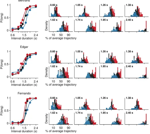
We trained three rats to categorize time intervals as either long or short by making left/right choices (figure 2.1; see section 2.4.1 on page 35 for full description). In brief, animals initiated trials by inserting their snout in a centrally located initia-tion nose port, thus triggering the presentainitia-tion of a stimulus. Stimuli consisted of two brief sound tones separated in time by an interval randomly selected from the set I = {0.6,1.05,1.26,1.38,1.62,1.74,1.95,2.4} seconds. Judgments about interval du-ration were reported at two laterally located nose ports: choosing the left side was reinforced with a drop of water after intervals longer than 1.5 seconds, and the right side otherwise. Incorrect choices were punished with an error tone and a time out.
An-0.6 1.5 2.4
0 0.5 1
Interval duration (s)
P(long)
Average
0.6 1.5 2.4
Interval duration (s) Edgar
0.6 1.5 2.4
Interval duration (s) Fernando
0.6 1.5 2.4
Interval duration (s) Gabriel
0.0 s 0.6 s 1.5 s 2.4 s 3.0 s
Figure 2.3. Behavior displayed during stimulus interval is highly reproducible. A series of video frames taken from a representative session of rat Fernando at specific time points within trials were averaged across all presentations of the longest interval.
Times when frames were taken are indicated in seconds relative to interval onset. n= 62
trials.
imals were free to move during stimulus presentation, as long as they withheld choice until interval offset.
Each interval presentation followed by a choice constitutes one trial, and rats per-formed on average 453 trials per daily session (range = 346 to 558, standard deviation = 49.4). As revealed by their psychometric functions (figure 2.2), animals correctly cate-gorized the easiest (i.e., shortest and longest) stimulus intervals at a rate of 95.8±0.03%, while performance declined as intervals came closer to the 1.5 seconds categorical bound-ary reaching 69.4±5.58% for the most difficult stimuli; over all eight stimuli, 84.7±3.57%
of trials were categorized correctly (mean±standard deviation).
−0.5 0 0.6 1.5 2.4
−8.5 0 8.5
Time from interval onset (s)
Head
posit
ion
(cm)
Edgar
Fernando Gabriel
5
cm
−0.5 0 0.6 1.5 2.4
Time from interval onset (s)
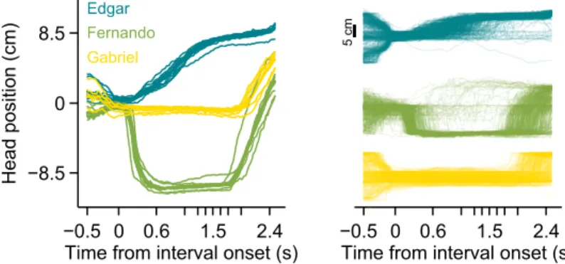
Figure 2.4. Head trajectories are reproducible and idiosyncratic. (left) Head trajectories around presentations of longest interval. Thin lines are single session means.
Edgar FernandoGabriel
Trial number
Trial number
1 624 1248
1 624
1248 1 Trajectory correlation
0
−1
Different subjects
Same subjects, different sessions
−1 0 1
Same sessions
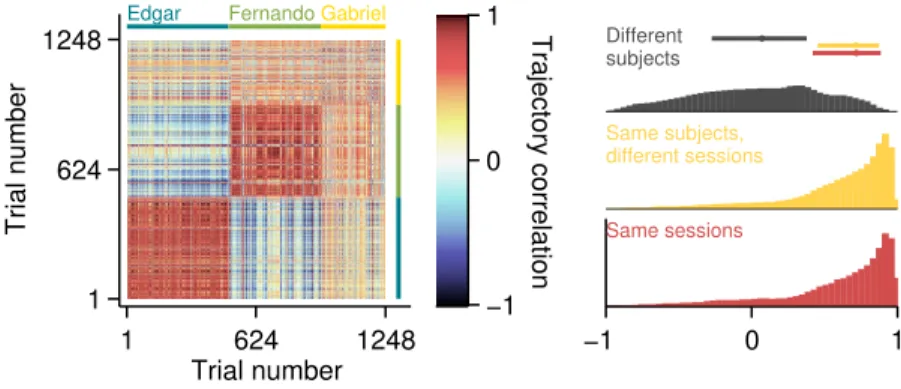
Figure 2.5. Pairwise correlations between head trajectories. (left) Matrix of pairwise correlations between trajectories shown in figure 2.4 on the previous page. Trials are ordered by subject (color bars framing top and right margins), then session,
then trial number. (right) Normalized histograms of correlation coefficients between
single trial trajectories from different subjects (dark gray), or from the same subject and in the same (yellow) or different (red) sessions. Dots and bars above histograms are medians and interquartile ranges. n={491,445,312}trials in {10,8,6}sessions from the three rats.
2.2.2
Animals developed temporally structured behavior
of each animal’s head in time (see section 2.4.3 on page 36 for details). In agreement with the example video in figure 2.3 on page 26, head trajectories revealed body motion patterns that were very consistent across trials, as well as across sessions (figure 2.4 on page 26). Interestingly, each subject developed its own distinct trajectory.
To assess the within and between subject variability in head trajectory, we computed a correlation matrix comparing all pairwise combinations of trials wherein the longest interval duration was delivered (Figure 2.5, left). Correlations between trajectories produced by a given subject were highly and consistently positive, whether or not they occurred in the same session (Figure 2.5, right; distributions of correlation coefficients
are indistinguishable, Kolmogorov-Smirnov test,p= 0.84). Trajectories from different
subjects, on the other hand, were uncorrelated on average, and the distribution of
coefficients differed significantly from both within subject distributions (K-S tests,p=
9.7×10⁻⁴ in both cases).
Given the observation that trajectories are idiosyncratic and consistent from session to session, we pooled data across sessions within subjects for the following analyses.
2.2.3
Ongoing behavior bears information about unfolding
perceptual decisions
Next, we asked whether trial-to-trial variability in body trajectories carried information about the perceptual decisions being forged; were this the case, different categorizations of the same stimuli should be accompanied by distinct behavioral trajectories. For a representative session of rat Edgar, we selected all presentations of the stimulus for which choice variance (σ2choice) was highest (I= 1.38 seconds;n= 56 trials;σchoice2 = 13.3571). The different color channels in the video were used to parse trials by choice: long choice
0.00 s 0.46 s 0.96 s 1.38 s 1.84 s
−0.5 0 0.6 1.5 2.4 −8.5
0 8.5
Edgar
−0.5 0 0.6 1.5 2.4 Fernando
−0.5 0 0.6 1.5 2.4 Gabriel
Figure 2.7. Head trajectory is predictive of choice. Average head trajectories lead-ing to long (blue) and short (green) categorizations of same near boundary durations. Gray shaded area indicates stimulus interval period. For each subject, the stimulus of highest choice variance across sessions was selected. Red bars indicate moments when head position is significantly predictive of choice (95% bootstrap confidence intervals
on area under the receiver operating characteristic (ROC) curve). n={678,475,300}
trials.
trials were put in the red, and short choice trials in the green channel. The resulting video reveals a separation in body position since the first few hundreds of milliseconds (Figure 2.6 on the preceding page).
The differences in behavioral trajectories leading to different categorizations of the same stimuli imply that it should be possible to predict choice from behavioral tra-jectories. To quantify this effect, we employed a metric commonly used in sensory
neuroscience known aschoice probability (Britten et al., 1996; Nienborg, R. Cohen, &
Cumming, 2012). Choice probability is defined as the degree to which fluctuations of a variable during repeated presentations of a stimulus are predictive of perceptual judg-ments about that stimulus. This metric is commonly applied to the firing of neurons in sensory brain areas in order to estimate their involvement in the formation of per-cepts (Parker & Newsome, 1998). We extend its use to assess whether body trajectories carried information about unfolding perceptual judgments of time intervals.
(Green, Swets, et al., 1966). This curve was calculated using head position distributions for data from short versus long choice trials (see section 2.4.4 on page 37 for details). In agreement with the example video, this analysis revealed that overt behavioral se-quences often allow perceptual judgment to be predicted above chance. The profile of choice probability over time differed for each individual subject (figure 2.7 on the previous page). Edgar displayed a monotonically increasing profile that was significant from before stimulus onset and throughout stimulus presentation. Fernando displayed a more complex profile that was significant early in the stimulus, lost significance, and
then regained small but generally significant separability from ≈0.7 seconds onward.
Gabriel did not display overt head trajectories during the interval period, staying at the initiation port throughout presentation of the stimulus interval instead (see figure 2.4 on page 26). However, Gabriel’s choice probabilities were significantly greater than chance prior to trial initiation. The absence of appreciable change in Gabriel’s head position during the interval period made it impossible to extract any information from this variable. However, close inspection of individual videos suggested that this rat may have produced smaller scale movements around the initiation port in the axis normal to the image plane. We were not able to quantify such movements using the current setup, and thus likely underestimated the degree to which this animal’s movement may have related to choice.
The analysis of head position presented in figure 2.7 on the previous page represents a behavioral analogue of instantaneous neuronal choice probability, calculated during the presentation of near boundary stimuli. The following analysis differs in that it assesses the predictive power of a 1-second long segment of the head trajectory with regard to choice across different difficulty levels.
Briefly, the trajectory described by head position on trialkduring a time window
extending from 0.5 seconds before trial initiation to 0.5 seconds after was represented
as a vectorhk. Since the shortest possible stimulus duration is 0.6 seconds, this period
is identical across all trials in the sense that no information about stimulus duration has been presented. Intuitively, if behavioral trajectories are systematically related to
perceptual decisions, head position vectors hobserved on long and short choice trials
should form separable clouds.
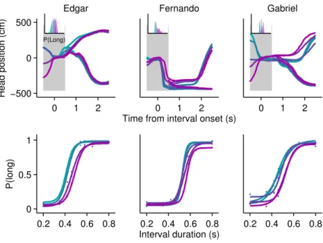
All psychometric curves asymptoted near 0 and 1, but biases were strikingly different and ordered. As noted, this analysis took as input behavior occurring before stimulus identity could possibly be known by the subject. Importantly, the ordered psychometric functions do not suggest that the animal has already made its decision prior to stimulus presentation. Were this the case, performance should be at chance level. Rather, the animal’s head trajectory exerted a bias on choice, as the difference in psychometric functions was mainly captured by the bias parameter. The same pattern would be expected if we could bin trials with respect to internal decision variables such as clock speed or decision criterion.
2.2.4
Behavioral trajectory improves choice prediction
be-yond trial history
The average head trajectories during the period preceding trial initiation were strikingly related to choice probability (Figure 2.8 on page 41, top panels). This suggests that the predictive power of trajectories reflected events preceding the current trial, such as choices made and rewards received on recent trials (e.g., Sugrue, Corrado, & Newsome, 2004; Lau & Glimcher, 2005). To test whether behavioral trajectories significantly improved our ability to predict choice beyond the information provided by trial history, we fit four logistic regression models to the choice data that differed in the combination of predictor variables included. We allowed different combinations of subject, current trial stimulus, recent trial history of choices, stimuli and rewards, and head trajectory to be weighed in predicting choice (see section 2.4.5 on page 38 and Table 2.2 on page 39 for details).
Model #1 captured the effect of stimuli, expected to be strong if animals learned the duration discrimination rule inherent in the task. Dummy variables standing for individual subjects were used to capture cross subject differences in psychometric func-tions. As expected, model #1 predicted choice at a high success rate (Table 2.1 on page 33), and was strongly significant as compared to a constant model (log likelihood ratio test,χ2= 6.01
·103, df= 5, pwithin rounding error of 0).