M
ASTER IN
F
INANCE
M
ASTER
’
S
F
INAL
A
SSIGNMENT
D
ISSERTATION
P
AIRS
T
RADING PERFORMANCE AND IMPLICATIONS APPLIED TO THE
P
ORTUGUESE MARKET
F
RANCISCO
C
ASTELO
B
RANCO
M
ASTER IN
F
INANCE
M
ASTER
’
S
F
INAL
A
SSIGNMENT
D
ISSERTATION
P
AIRS
T
RADING PERFORMANCE AND IMPLICATIONS APPLIED TO THE
P
ORTUGUESE MARKET
F
RANCISCO
C
ASTELO
B
RANCO
O
RIENTATION
:
R
AQUEL
M.
G
ASPAR
Pairs Trading Performance and Implications Applied to the
Portuguese Market
Francisco Castelo Branco†
Technical University of Lisbon
September 2012
Abstract
Pairs trading is a statistical arbitrage strategy that gains popularity on Wall Street in the mid-1980's. Such concept is actually very simple to understand: select two assets that had a closely past behavior and when that path is disturbed, take a long/short position in the hope that in the future, history repeats itself. Thus, the primary aim of this final master thesis is to explore and analyses the effectiveness of implementing such strategy in the Portuguese stock market during the period comprised between 2002 and 2012. Since Pairs Trading strategy only uses past stock information and the Efficient Market Hypothesis in its weak-form, states that stock prices already contain all historical data available on the market and therefore, there is no way of using that information in order to produce excess risk adjusted returns, the second objective of the thesis is to confirm that Pairs Trading do in fact explore market inefficiencies to generate statistical excess returns over the market, and present new evidence about the informational efficiency of the Portuguese stock market. This research verifies which value of the thresholds and what method maximises the strategy profitability. It also verifies the importance of that threshold and necessity of an accurate selection of the pairs on the strategy performance.
JEL
: C22; C32; G11; G12; G14;
Keywords
: pairs trading, statistical arbitrage, quantitative strategy, market
efficiency, cointegration, Portuguese stock market.
Pairs Trading Performance and Implications Applied to the
Portuguese Market
Francisco
Castelo Branco
1 Technical University of LisbonSeptember 27, 2012
1Technical University of Lisbon-School of Economics and Management (ISEG), Student of Masters in
Contents
1 Introduction 4
2 Literature Review 7
3 Data 13
4 Methodology 15
4.1 Pairs Formation . . . 15
4.1.1 Square Distance Approach . . . 15
4.1.2 Cointegration Approach . . . 17
4.2 Returns Computation . . . 18
4.3 Transaction Costs . . . 20
4.3.1 Explicit Costs . . . 20
4.3.2 Implicit Costs . . . 20
4.4 Assessing Pairs Trading Performance . . . 21
4.5 Efficiency Tests . . . 22
5 Results 23 5.1 Square Distance Approach . . . 23
5.2 Pairs Trading under differentd . . . 26
5.3 Assessing Pairs Trading Performance . . . 27
5.4 Efficiency Tests . . . 27
5.5 Cointegration Method . . . 29
5.6 Updated Data - The first 3 Quarters of 2012 . . . 31
6 Conclusions and Implications 33
References 35
List of Figures
4.1 Pairs at the Selection Period . . . 16
4.2 Pairs at the Trading Period . . . 17
5.1 Volatility . . . 23
5.2 Pairs Trading Portfolio versus Market Performance . . . 24
5.3 Pairs Trading Portfolio Annual Returns . . . 25
5.4 Pairs Trading and the Issue of Luck Analysis . . . 28
5.5 PSI-20 and the Issue of Luck Analysis . . . 28
5.6 Pairs Trading Portfolio Annual Returns . . . 30
List of Tables
3.1 List of Financial Stocks used in this Research . . . 13
7.1 Stock’s Pairs Over the Time . . . 38
7.2 Pairs Trading Returns per year . . . 39
7.3 Pairs Trading and Market Returns . . . 39
7.4 Apha and Beta for Pairs Trading . . . 40
7.5 Pairs Trading Summary Statistics . . . 40
7.6 d Value Sensitivity Analysis . . . 41
7.7 Summary Statistics for Pairs Trading under differentd . . . 41
7.8 Random Trigger Test . . . 42
7.9 Random Trigger OLS Analysis . . . 42
7.10 Random Pair Test . . . 43
7.11 Random Pair OLS Analysis . . . 43
7.12 Run Test . . . 44
7.13 Autocorrelation Test . . . 45
7.14 Cointegration method Analysis . . . 46
1.
Introduction
In the financial markets there have been, for a very long time, numerous investment strategies that tried to make profit out of the market inefficiencies and anomalies. A cluster of such strategies, known as quantitative analysis or statistical arbitrage, tries to take advantage of short term detour from the “fair” asset price to generate statistical excess returns through sophisticated techniques and effective algorithms. Pairs Trading is a strategy enclosed in this type of statistical arbitrage and widely practice by hedge funds. The two major attractive characteristics of the strategy are its neutrality to the market, in sense that it generates a zero beta over it, and its effectiveness on exploiting the market inefficiencies to generate excess returns.
The efficient market hypothesis (EMH),in its weak form, postulates that the past available infor-mation of an asset is entirely incorporated on the asset value. This means that by only taking into account historical data, there is not any potential on predicting the future behavior of an asset price. The consequence of such hypothesis is that there is not any logical trading rule, based only on past information, that could generate a significant positive excess return over the market. Considering all of that, it is interesting to assess if in practice it is possible to generate systematically positive excess returns by conducting one statistical arbitrage strategy as it is Pairs Trading.
Pairs Trading is framed with quantitative strategies presenting as the main glamour its low risk due to the expected non correlation to the market behavior, and its high positive performance owing to the consistent returns. When money is at stake in the financial markets, “Human beings do not like to trade against human nature, which wants to buy stocks after they go up not down1”. By contrast, in Pairs Trading and in the majority of statistical arbitrage strategies, the idea is to sell assets that are overvalued and buy the ones that are undervalued, when analysed and compared with its “fair” value. Obvious the “fair” value is not an easy thing to determine and due that reason, Pairs Trading does not base the strategy on assessing the “fair” value of an asset, but else, on the relative pricing. The idea of relative pricing is sustained upon the notion that assets with similar characteristics should present, more or less, the same value. Thus being, when the value of two similar assets present different prices, it is possible to assume that, one or both, are overvalued or undervalued relative to its “fair” value.
Pairs Trading might be a concept of widespread understanding, yet very complex to implement. The process is based on identifying, with high accuracy, assets that had similar historical behavior and trade them when the correlation deviates, shorting the higher value asset and buying the lower value asset. By exploring such spreads they create a valid possibility of making profits when, eventually, the assets revert to moving together. The two most important phases in order to achieve success in this strategy are the one of identifying the pairs and the one of implementing an efficient trading algorithm. There are some typical aspects and questions regarding Pairs Trading implementation that are enlightened in this Thesis. For instance, which assets should be designated to be pairs? What distance deviation between the pairs is good enough in order to initiate the trade? When is that the trade is closed? And what if it never closes? In order to go dipper than the usual questions, it is important to conclude with proper proof that Pairs Trading is not an issue of luck, rather an efficient strategy.
From academic literature it is possible to define four distinctive methods for implementing Pairs Trading.(i) Gatev et al. (2006), introduces the minimum distance method based on the distance relation of two normalised assets; (ii) Nath (2006) and Elliott and Malcolm (2005) outline a stochastic approach to a spread by modeling its behavior of mean reversion; (iii) Combined Forecast approach which is given by Huck (2009,2010) and does not assume any equilibrium model and; (iv) Finally, Vidyamurthy (2004) outlines the cointegration approach, that tries to parametrise the strategy.
This Thesis covers both the Minimum Distance and the Cointegration methods. Although the methods are used in some literature, there exist specifications that are not always obvious. For that reason, the undertaken methods follow the original works whenever it is possible but also take certain assumptions without undermining the essence of the methods. Such essence is the same in both methods: the selection of the pairs is done using only historical data; and the trigger of the trade as well as the positions to take are always based upon a spread process behavior.
The purpose of this Thesis is to analyse Pairs Trading under the concepts of Minimum Distance and Cointegration methods and derive the dynamic implications of it on the balance of price series, this is, the evaluation of the mean reversion on the pairs strategy. Thus, after implementing both strategies, the aim of the Thesis is to assess the profitability and implications of Pairs Trading applied to the Portuguese index market (PSI-20).
market. First, Pairs Trading is relatively known in the trading sphere but it did not have the same attention nor the same rigorous analysis when compared with momentum or contrarian investment strategies. Second, since it is a market neutral and self-financing strategy, it is interesting to observe if it is possible to obtain better results than the market and verify which of these results are due to the behavior of the market and what part is due only to implementation of the strategy. Finally, since Weak-Form efficiency is based on the premise that past stock prices can not be used to generate alpha i.e. informational efficiency states that no one can get an alpha2 different from zero using any past information, this thesis also provides evidence on the informational efficiency on Portuguese stock market.
2.
Literature Review
Any strategy is considered neutral to market returns when their strategy returns are not correlated with market returns. A market neutral strategy follows its own path regardless the market movements. If a strategy is uncorrelated with the market, in the CAPM1context, it means thatβ is equal to zero. It is intuitive that market neutral strategies are able to eliminate the systematic risk2. Pairs Trading, as said before, gained popularity among the hedge funds due to the ability of profiting through the anomalies in the financial markets but also due to its independence from the market actions.
Jacobs et al. (1993) affirms that in order to eliminate the exposure to the market risk, a portfolio should use a long-short strategy to become a zero beta portfolio and achieve returns only by its alpha. Such strategy may be called a market neutral strategy. This statement is also sustained by Fung and Hsieh (1996) where it is defended that a strategy that generates returns independently from the market returns may be called as neutral. Long-short market neutral strategies, as Alexander and Dimitriu (2002) states, displays no correlation with the market, lower volatility and, at most of the time, presented better Sharpe Ratios than the market index.
In order to construct a market neutral strategy it is imperative to have a zeroβ portfolio. Vidya-murthy, G.(2004) demonstrates that it is possible to do that by holding both a long and a short position on different stocks. Consider thatrA as the portfolioAreturns, rB as the portfolioB returns andr
as the ratio3:
rA=βA∗R(M) +θA (2.1)
rB =βB∗R(M) +θB (2.2)
So as to initiate the trading strategy, it is establish ther units ofAas being the portfolio to short and one unit ofB as the one to buy,
rAB =−r∗rA+rB (2.3)
rAB =−r∗(βA∗R(M) +θA) +βB∗R(M) +θB (2.4)
1Capital Asset Pricing Model, firstly proposed by William T. Sharpe (1964), Jack Treynor (1961, 1962), John Lintner
(1965) and Jan Mossin (1966).
2Market Risk 3β
rearranging the terms,
rAB = (−r∗βa+βb)∗R(M) + (−r∗θA+θB) (2.5)
knowing thatr representsβB/βA the combined portfolioβ is equal to:
βAB=−r∗+βA+βB= 0 (2.6)
as we wanted to prove.
Statistical arbitrage4strategies are created in order to explore the inefficiencies of the market and therefore eliminate the exposure to the market. Minimizing such exposure will traduce on eliminating the β and conferring to the strategy returns non correlation to the market returns. Jarrow et al. (2003) mentioned that statistical arbitrage strategies, by definition, follow four conditions: (i) self-financing or zero initial costs; (ii) positive expected profits; (iii) probability of loss converging to zero and; (iv) time average variance also converging to zero. All the prior conditions automatically imply that such strategies will produce riskless incremental profit and positive Sharpe Ratio. In fact, the notion of statistical arbitrage does not support the idea that market is in an economic equilibrium. As is supported in Jarrow (1988) this economic equilibrium is an essential premise for an efficient market. The efficient market hypothesis5 has been discussed for decades and was developed by Eugene Fama (1965,1970), Cootner (1964), Samuelson (1965), Roberts (1967) among many others in the early 1960s. EMH considers that financial markets are informational efficient and therefore it is not possible to consistently achieve excess returns on the market given the information available, at the time the investment is made. Moreover Jensen (1978) stated that market efficiency with respect to an information set,ϑ, implies that it is impossible to make economic profits6 by trading on the basis of
ϑ.
Efficient Market Hypothesis, as explained in Fama (1970), claims that a stock price should both reflect the true value of a stock and also all the available information. Those statements imply that there is not any opportunity of arbitrage in a rational economy.
Stocks expectations can be defined by:
E(Pi,t|Φt−1) = [1 +E(ri,t)|Φt−1]Pi,t−1 (2.7)
4More details on the terminologies can be found on Khandani and Lo (2007). 5Now on referred as EMH and referring to its weak form.
where,E is the expected value,Pi,t is stock’s price in the periodt,ri,t represents the return of the
stocki during periodt, and Φt−1 is the set of information presented on the market at timet-1. The
left-hand side of the equation exhibits the expected price of stocki given the information available at the timet-1. On the right-hand side, the expression denotes the expected return of stocks having an equal risk to stocki.
Now consider thatxi,t accounts for the difference between the price of a stocki at timet and the
expectation that an investor had at timet-1 of that stock for the next period:
xi,t=Pi,t−E(Pi,t|Φt−1) (2.8)
considering that in an efficient market: E(xi,t|Φt−1) = 0, it is possible to infer that the information is
always incorporated in stock prices and therefore the potential expectation of a stock return, according with EMH, may be represented as: Pt=Et−1Pt+εt. Underlying the efficiency market hypothesis, it
is opportune to mention that expected stock returns are entirely consistent with randomness in assets returns (Samuelson (1965)).
Informational efficiency holds on the market capacity of replicate, almost instantaneous, the fi-nancial reliable information on the asset prices. The Random Walk Hypothesis (RWH) is about independent and identically distributed (i.i.d.) of the increases, in which the price formation should be:
Pt=µ+Pt−1+εtεt∼idd(0, σ
2), (2.9)
whereµis the expected variation of the price. According to Lucas (1978), the major difference between RWH and EMH is the risk-return trade-off. Although it is not entirely true to affirm that RWM tests can conclude about the market efficiency, those can provide valid information about weak-form efficiency questions.
Nevertheless, there exists a lot of empirical studies that seems to contradict the EMH. Jegadeesh and Titman (1993), using one trading strategy that only uses historical well and poor performing assets, obtained an excess return of 12% per year. A similar conclusion was found by Lakonishok, Shleifer, and Vishny (1994) when using historical value versus historical glamour. Coval, Hirshleifer and Shumway (2005) found evidence that the investor’s persistent abnormal returns were not due to inside information, rejecting therefore the EMH. Another study that founds violations of the EMH is the research of Cahn, Jegadeesh, and Lakonishok (1996) where it is confirmed that a strategy based only on past returns and earning announcements provide future excess returns.
EMH is, after all, only a hypothesis not a proven fact, nor it is its rejection. So many years had passed since the introduction of this hypothesis and there is still no consensus amongst researchers. About the present research, EMH is tested on the principle that: given a market and a set of infor-mation about both the market and the assets that belong in it, EMH affirms that those assets prices are at its fair price given that information; obvious the significance of such premise is that there is no way of using that information in order to produce excess risk adjusted returns, meaning that it is not possible to beat the market performance.
Among the quantitative or statistical arbitrage, Pairs Trading is a very popular strategy being used by hedge funds and investment banks but still not widely notorious as momentum and contrarian trading strategies. Such concept is actually very simple to understand: (i) Find two stocks with both historical similar characteristics and correlated paths; (ii) when the path of those stocks is disturbed and the spread between them is higher than ”d”7 a trading signal is created; (iii) sell the stock with the higher value and buy the other one; (iv) if history repeats itself, and both prices converge, the open positions are closed and profit will be made8.
It all begun in the 70’s at Princeton-Newport Partners, an investment company founded by the mathematical financier Edward Thorp (Ed Thorp), who was a fervent advocate of markets inefficien-cies. Overwhelmed with proofs of such, he decided to verify how inefficient the market was and how it would be possible to exploit profits from that. The answer came from the statistical arbitrage toolbox and the idea was to rank the stocks performance and thus construct a market neutral portfolio by taking long and short positions on the most down and most up stocks, respectively. Ultimately due to the good performance of Princeton-Newport Partners, the idea was left behind. Disconnectedly from
7The value of ”d” is not a value stipulated by rule but arbitrary decision of the investor.
8When the prices converge, according to logic, the shorted stock will reduce the value and the other will increase the
the work that was developed by Ed Thorp, in the early 80’s at Morgan Stanley9, Gerry Bamberger developed another statistical arbitrage scheme similar but at the same time less variable than the Ed Thorp’s. Although the initial phase translated into significant profits, it was never implemented as a major strategy on Morgan Stanley. Displeased with the non-recognition of his work, Gerry Bamberger left Morgan Stanley and Nunzio Tartaglia, come up with a team in order to improve and explore the strategy and new possibilities of profit trough quantitative arbitrage strategies. Such team was composed by mathematicians, physicists and computer scientists. The result of their study was the Pairs trading. Since the first time that it was applied, such strategy has become very popular in the investment banks and hedge funds sphere.
Pairs Trading is a strategy where the ”human subjectivity had no influence whatsoever in the process of making the decision of buy and sell a stock” (Perlin, M. (2009)). The first empirical work referring this strategy is attributed to Gatev, Goetzman and Rouwenhorst (1999) where it was documented an analysis of Pairs Trading strategy and how it affects the theory about market efficiency. Few years after Gatev et al. (2006) upgrading the original work, with more recent data, it was found proof of considerable profits uncorrelated to the S&P 500.
Gatev et al. (2006) is the most cited paper regarding Pairs Trading. The identification of the pairs is elaborated by using the distance method10. Such method was also used by Do and Faff (2009), Perlin (2009), Bolg¨un, Kurun and G¨uven (2009) and Do and Faff (2011) when testing the performance of Pairs Trading. Perlin (2009), when examining Pairs Trading on the Brazilian market concluded that the strategy had a good performance, returns not correlated with the market and the strategy,in fact, took advantage of the market inefficiencies. Bolg¨un, Kurun and G¨uven (2009) affirmed that the strategy produced powerful returns especially during volatile periods. Finally Do and Faff (2009), when extending Gatev et al. (2006) work stated that although profit was declining such fact could be avoided if pairs were calculated more often. More recently Do and Faff (2011) introduced accurate transaction costs and concluded that although the disappearing of high profits, Pairs Trading still presents positive returns and low risk.
However, there are others models to identify the pairs through more rigorous tests and forecasts. The cointegration approach drawn in Vidyamurthy (2004) is an attempt of parametrise Pairs Trading, by exploring the possibility of two time series, with integration of the same orderd, could be linearly matched in order of generating a single time series integrated of order d-b, with the condition that
b>0.
The notion of cointegration emerged with Engle and Granger (1991) by explaining that unlike correlation, cointegration is a measure of long-term dependencies. Facing the perspective of having to work with non stationary time series it is more thoughtful trying to construct portfolios that can be related to stationary time series. Such approach is highly recurrent among all asset classes and accomplished by cointegration techniques.
Engle and Granger (1991) states that two time series, xt and yt, are cointegrated if, and only if,
each is I(1) and a linear combinationxt−α−βyt, whereβ16= 0 is I(0).
3.
Data
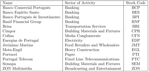
The data consists on the 14 most liquid stocks of the Portuguese stock market, PSI-20. Such list can be viewed in Table 3.1.
Table 3.1: List of Financial Stocks used in this Research
Name Sector of Activity Stock Code
Banco Comercial Portuguˆes Banking BCP
Banco Esp´ırito Santo Banking BES
Banco Portuguˆes de Investimento Banking BPI
Banif Financial Group Banking BNF
Brisa Transportation Services BRI
Cimpor Building Materials and Fixtures CPR
Cofina Media Conglomerate CFN
Energias de Portugal Electricity EDP Jer´onimo Martins Food Retailers and Wholesalers JMT
Mota-Engil Heavy Construction EGL
Portucel Paper PTI
Portugal Telecom Fixed Line Telecommunications PTC Semapa Building Materials and Fixtures SEM ZON Multim´edia Broadcasting and Entertainment ZON
Liquid stock means that in the period of analysis it had at least 90% of valid close prices. This criteria is crucial since the lack of liquidity of the stocks is an enormous risk when implementing Pairs Trading strategy. This risk is characterized by higher costs as bid-ask spread and the difficulty of having short positions opened for more than 3 days.
The data, from 2002 until 2012, was obtained through Datastream and adjusted for splits and dividends on a daily frequency. Note that, when choosing the stocks to consider, they were filtered in order to only choose those that were listed during the all period.
Portuguese stock market is less liquid then the American and also composed by less stocks, which could constitute a problem. Since the study lies on the Portuguese market, PSI-20, and as Alexander et al. (2002) shows, efficient long short hedge strategies can be achieved with relatively few stocks, therefore this potential problem is ignored.
if they obey to the establish criteria.
4.
Methodology
4.1
Pairs Formation
From academic literature is possible to identify 4 methods of pairs selection. The first one is the Square Distance approach implemented on the works of Gatev et al.(1998,2006) and Do and Faff (2003) among others. As it is explained with more detail on the next section, this approach merely searches a statistical relationship within pairs. The second major approach is know as Cointegration approach which incorporates the mean reversion on Pairs Trading structure, simply the most significant statis-tical relationship in order to succeed. Such approach is introduced on the researches of Vidyamurthy (2004) and Alexander and Dimitriu (2002) inter alia. Those two approaches mentioned above are the two methods that are included and tested in this research. Finally the last two approaches mentioned on the literature are the Stochastic and the Combined Forecast approaches. The first one is included in Elliot et al. (2005) and Do et al. (2006). Such approach models the mean reversion behavior of the spread and is widely defended due to the ability of capturing it on a continuous time model and with parameters easy to estimate. Nevertheless this approach have a fundamental limitation on restricting the long run relationship of two pairs to one of return parity (Do et al. (2006)). The last approach is encouraged by Huck (2009,2010) given that provides more trading chances. Such approach differs from the others since it does not make any reference to an equilibrium method.
4.1.1
Square Distance Approach
It is essential that the price series pass through a normalisation procedure,Pn= Pi−E(Pi)
σi , so that
they are brought to the same standard unit in order to permit a quantitatively fair choice of the pairs. This procedure is very important in order to avoid the impossibility of setting a distance trigger1 on the pair. After this procedure, using the minimum distance rule, presented on Equation(4.1), each stock respective pair that minimises the square difference between the normalised prices is searched.
M in(
t
X
1
Pin− t
X
1
Pjn)2, i= 1,2, ..., n∧j= 1,2, ..., n∧i6=j (4.1)
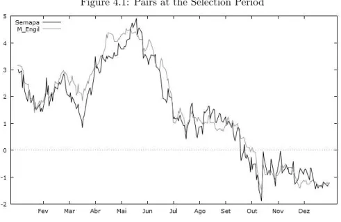
As Gatev et al. (2006) points, pairs traders normally search for two stocks whose prices followed the same patterns. This suggests that square distance approach is the most similar to how traders find their pairs. That said, the minimum distance approach will be used to match stocks with their pairs as shown in Figure 4.1.
Figure 4.1: Pairs at the Selection Period
Afterwards is important to set the distance,d, that will trigger the trade. dvalue, as referred before, is arbitrary to the investor will. Nevertheless its important to take into account some considerations: (i) if the value ofd is very high probably no trade will take place (ii) if the value ofdis very low, there will be a significant number of transactions increasing the transaction costs. Hereupon the value ofd
will be 2 standard deviation2, meaning that every time the absolute distance3 is higher than 2 a trade will take place4. Although this value of 2 standard deviations is used as standard, it is also interesting to test other values to unleash the trade. Having in mind all the considerations, this research verifies such ideas by exploring the results of exercising the strategy with differentd.
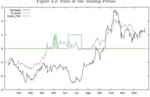
Note that also in order to be a self-financing and market neutral strategy, there will always be a ratio, Pb/Pa, to confer the same weight to both bought and sold assets. The Figure 4.2 shows the
behavior of one pair during trading period and the respective trades that are opened.
2This value is the most common on the literature and therefore, before analysing which value maximises the strategy,
this 2 standard deviation value is used as default.
3By absolute distance it is meant the spread.
Figure 4.2: Pairs at the Trading Period
4.1.2
Cointegration Approach
The main challenge in this type of strategies is to identify the stocks that tend to move together over time and therefore make potential pairs. It is known on advance that if an asset price series is stationary it will respond with success to a mean reverting strategy. But we also know that asset price series are not stationary. Nevertheless we can build a stationary series with two cointegrated asset time series. Cointegration theory is definitely an innovation in theoretical econometrics. Unlike correlation, it does not refer to the co-movements in returns but to co-movements in raw asset prices. Letyt andxtbe two nonstationary time series. If in a certain moment ofy, the series yt−γxtis
stationary we can say that y and x are cointegrated. The idea behind cointegration is that y and x
have a long-run equilibrium that when disturbed from the long-run mean it is expected that, one or both time series, adjust and return to the equilibrium.
Given a time series that is not stationary and only stationary after differingn times can be called ”integrated of ordern”, denoted I(n). Consider a random walk,yt=α+yt−1+εt, is a I(1) whereα
denotes the drift and the error processεtis i.i.d. stationary process. Said that,x andy are cointegrated
By definition axtseries is I(1) if the first difference is stationary, I(0). Consideringx1t, x2t, ..., xkt
a time series I(1); if there areβ1, β2, ..., βk 6= 0 such that β1x1t, β2x2t, ..., βkxkt results in one series
I(0), thanx1t, x2t, ..., xkt are said to be cointegrated5.
Assuming a long-short position in two time series that are not cointegrated it is possible that the value of the pair is stationary, meaning that they are cointegrated. If the time series is stationary, one strategy based on mean reverting is profitable, at least until the stationary status is not interrupted.
Applying the cointegration idea on the Pairs Trading analysis in order to detect potential pairs: (I) Using the Augmented Dikey Fuller test, we verify if all asset time series are I(1); (II) After confirming the nonstationary status of the time series is used a Engle-Grager or a Johansen test on all possible combinations to verify which pairs are cointegrated; (III) Having the pairs it is formulated a linear combination between the two time series to obtain theβ of the regression.
In order to start the strategy it is also necessary do calculate the spread between the time series,
Pxt−βPyt=Zt (4.2)
where β is the cointegration coefficient and Zt is the value of the spread over time. The spread is
mean reverting giving that both time series are cointegrated. Having already the spread it is done a normalisation procedure by its historical mean and standard deviation. Once again it is indispensable to settle the rule to trigger the trade: sell (buy) the spread every time it deviates above (below) two standard deviation of the mean and close the trade when the spread reverts to less than 1 standard deviation of the mean.
4.2
Returns Computation
In order to conclude if the strategy created value and be able to take conclusions about Pairs Trading it is necessary to calculate the total return of the strategy. The following equation represents the raw return of the strategy,Rraw.
Rraw= T
X
t=1
n
X
i=1
ln( Pi,t
Pi,t−1
)Pi,tLS (4.3)
where,
T = Number of observations in the period;
n= Number o stocks considered in the period and;
PLS = Dummy variable that takes the value of 1 for a long position and -1 for a short position.
Such equation means that each time the strategy opens a position, the raw return return is Ri,t =
ln(Pi,t/Pi,t−1),i∈1, ..., n, controlled by the dummyP
LS that confers the position on the market.
Although the results of the whole strategy are considered as being before transaction costs, it seems
convenient to include them on the formula:
RT c=ln(1−c 1 +c)(
T X t=1 n X i=1
T ci,t) (4.4)
where,
c= transaction cost per trade and;
Tc= Dummy variable that takes the value of 1 if a transaction is made and 0 otherwise. joining both equations,
R=ln(Pi,t/Pi,t−1) +ln(
1−c
1 +c)⇔ (4.5)
⇔R=ln( Pi,t(1−c)
Pi,t−1(1 +c)
)⇔ (4.6)
⇔R=Ri,t+RT c (4.7)
But as it was explained before, Pairs Trading strategy always performs a transaction with a long and a short
position in two different assets, the stock and its pair. Said that, next equation incorporates this long-short
position on the returns computation:
RLST = T
X
t=1
"Xn
i=1
ln( Pi,t
Pi,t−1
)Pi,tLS+ n
X
j=1
ln( Pj,t
Pj,t−1
)Pj,tLS
#
∗(d)+ln(1−c 1 +c)(
T X t=1 n X i,j=1
T ci,j,t),
i6=j;
ifPLS
i,t = 1⇒Pj,tLS=−1;
ifPLS
i,t =−1⇒Pj,tLS = 1.
(4.8)
where,d=
1 if Absolute(Pint−1−P
n jt−1)
2>2σ
0 otherwise
Note that it refers to the case where it is used the
Mini-mum Distance Method. If it is performed the Cointegration Method,d=
1 if Absolute(Pit−1−βPjt−1)>2
4.3
Transaction Costs
When working with strategies that involve trading stocks it is important to have in mind the impact coming
from the transaction costs. Such term can be viewed as a necessary loss while pursuing the potential gains.
Nevertheless it is a topic that concerns each type of investor at a different level. Once Pairs Trading is based on
trading stocks (both long and short positions), this concern might have impact on the strategy result depending
on who is trading.
Although transaction costs are thecost of carrying out a transaction by means of an exchange on the open market their value highly differ whether it is a small investor or it is an investment bank. For instance for a single small investor the transactions costs will have a great impact on the results since the trading scale will
not compensate the costs. But on the other hand, the impact of transaction costs for a hedge fund will not be
so critical as for the small investor. Hedge funds place huge amounts of trading orders and as consequence the
transaction costs have a lower impact on the final result of their trades. Finally, it is important to highlight
that for the investment banks the impact of the explicit transaction costs might be null. This consideration is
sustained by the fact that banks are indeed the market makers and therefore banks will not pay commissions
or fees for something that is done by themselves. In this present thesis, due to the difficulty of accounting
for correct transaction costs, the research pursues a theoretical point of view, assuming 0 transaction costs,
although it may not waive away much of the reality given the fact explained above.
There are explicit costs and implicit costs associated with this kind of strategies.
4.3.1
Explicit Costs
On this section there are two types of transaction costs: commissions and short selling costs. Commissions
are the fee paid to an agent or a trading company for the services of facilitating transactions between buyers
and sellers. Short selling costs comes from the procedure of selling an asset not owned by the investor with
the intention of have profit later when the asset is bought back at a lower price. The investor does not own
the asset, therefore he has to borrow it and that has a cost.
4.3.2
Implicit Costs
The implicit costs are the bid-ask spread. This cost is undoubtedly the most difficult to measure and has
a great presence on this specific strategy. There are three considerations to make about this theme in order
to explain exactly what is this cost about. Primary the bid-ask spread is he quantity by which the ask price
is exceeding the bid price. Such definition is in actual fact the difference between the highest and lowest price
to have in mind that if a stock is quoted on the market at 50 euros and at that time is placed a buy order to
the market, if the stocks tick size is 1 euros, the stock was in reality bought at 51 euros. Here it is described
a cost of 1 euros that when working with stocks quotes it is not considered and therefore it has impact on the
strategy results. Finally, consider that the stock and its pair, at a precise moment, diverge from the path by
two standard deviations and that trigger the trade. The one that is bought is the one that was losing value
and the one that is shorted is the one gaining value. The result of this finding is that it is more likely that a
stock is bought at the quoted bid price when it should be at an ask price and the other is shorted at the quoted
ask price when it should have been shorted at a bid. This inconsistencies also generate a bid-ask spread that
affects the strategy performance.
4.4
Assessing Pairs Trading Performance
The idea behind this section is to verify if Pairs Trading has any science or it is all due to an issue of luck.
Such analysis is performed in two different ways: (i) attribute random pairs and (ii) simulate random entries
to simulate the values thatd takes over the time.
In the first test, attributing randomly the pairs, it is possible to test the importance of realising, for instance,
the square distance method and then verify whether the trading performance is in fact due to the strategy or
is just an issue of luck. In the second test, there are simulated randomly entries and retrieved the median to
trigger the trade. Both analysis have a critical importance to verify the part of Pairs Trading strategy return
that is not due to mean reversion.
Testing the strategies mean reversion, the market neutrality and verifying the annual returns are the
major conclusions of this section. At the random pairs strategy there are used the actual stock prices vectors
and therefore the trade triggers when its normalised prices separates for more than two standard deviation
unit. Here the test relies on the importance of calculating the suitable pairs in order to explore the market
inefficiencies. At the random trigger strategy, the pairs are the most suitable, calculated by the minimum square
distance method, but the trade do not bases upon the deviation of the long-term relation of the normalised
pairs. Here the test lies on the importance of waiting for the divergence of the pairs behavior in order to
explore the mean reversion possible profit.
In brief the goal of such tests is to verify if Pairs Trading performance is due to luck or the strategy is able
4.5
Efficiency Tests
According to the efficient market hypothesis (EMH), in its weak-form, it is impossible to forecast future
prices or returns based on historical information. Thus, there should not be possible to find a situation where
exists a linear dependence of future returns in relation to past performances.
In order to provide evidence on the informational efficiency of the Portuguese stock market, this Thesis
have two different approaches: The Run test and the Autocorrelation test.
Also known as Wald Wolfowitz test6, the Runs Test is a nonparametric test addressed to the analysis of
the randomness hypothesis. A Run + (−) is a sequence of positive (negative) returns. The null hypothesis is
that the two elements + and−are independently drawn from the same distribution.
Such test is realised through the comparison of the obtained number of runs in the series of returns with
the expected number of runs,E(R). Under the null hypothesis, the number of runs in the sequence is a random
variable with a conditional distribution determined by the observation ofn+ positive values and n-negative values. The Run Test can be defined as: H0: the sequence was generated randomly; H1: the sequence was not
generated randomly and; with a test statistic:
Z= (R−E(R))/pvar(r), (4.9)
approximately a normal distribution, computed as:µ= 2n+n−
N + 1 andσ
2= (µ−1)(µ−2)
N−1 .
The main question that this test answers is if this series was generated from a random process, this is, if
the series follow the random walk model.
The Autocorrelation test, sometimes called aslagged correlationorserial correlation, examines the relation-ship between random variables within past periods and current periods, based on different ranges of lags. Such
test may be used to test the dependency or not of a time series but also to identify a suitable model if that series
is not generated randomly. The statistic testQ, known asBox Pierce is given byQk =n(n+ 2)Pnk=1 c ρ2
k
n−k,
where: H0: The data is independently distributed, meaning that, if there is any observed correlations in the data it would only result from randomness;H1: The data is not independently distributed and;cρkis the series
autocorrelation at lagk withh lags to test, such that:
c
ρk=
Pn−i
k=1(rk−µb)(rk+i−µb)
Pn
k=1(rk−bµ)
(4.10)
Note that the metricQk follows an asymptotic distribution when the process returns are i.i.d.. That being,
5.
Results
5.1
Square Distance Approach
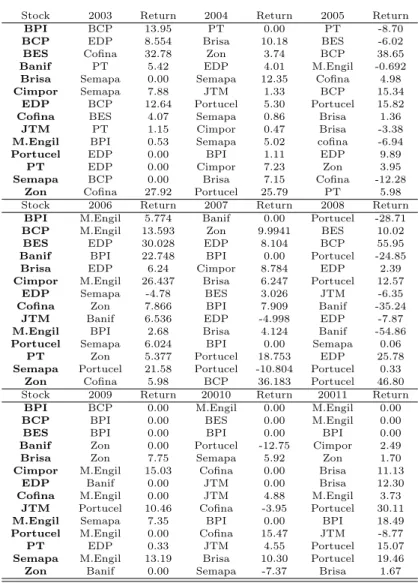
Table 7.1, presented on the next page, reveals the stocks and its pairs over the observation period. The
stock that over time was the most profitable wasBES1 earning more than 330%, representing about 37% per year. On the opposite side stands the stockMota Engil with losses on the order of -47%, meaning -5.24% per year. Another aspect that is possible to observe is that the stockBES had the same pair four times during the period whileBCP2, Cimpor, Cofina, Portucel andZon never held the same pair for more than one year.
The strategy performed encouragingly when compared to the market performance. Figure 5.1 and 5.2
replicate the volatility during the period and the accumulated returns, respectively.
Figure 5.1: Volatility
(i)Pairs Trading annual Volatility=8.40% (ii)Portuguese index Market annual Volatility=15.84%
From Figure 5.1 it is possible to observe that, as expected from a strategy like Pairs Trading, the volatility
is very low, lower than the market and also with a time average variance converging to zero. It is also possible
Figure 5.2: Pairs Trading Portfolio versus Market Performance
(i)Pairs Trading annual Return=10.91% (ii)Portuguese index Market annual Return=-0.88%
to enhance that the lowest observed volatility was on the year of 2009, year after the world crisis. Through
Figure 5.2 it is possible to verify that for about 75% of the study temporal horizon, Pairs Trading strategy
outperformed the benchmark3finishing the analyses period with a profit of 98.2%. Once again, Pairs Trading
distinguish form the Portuguese market during and after 2008, when it continued to achieve returns as if there
had been no crisis whatsoever unlike the Portuguese index Market that accumulated huge losses. In brief, the
both annual return and the annual volatility were, respectively, 10.91% and 8.4% for Pairs Trading strategy
and for the benchmark -0.88% and 15.84%.
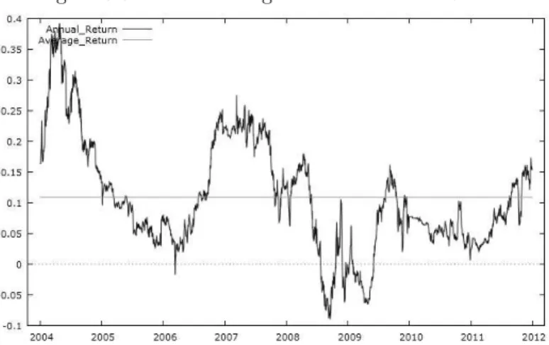
For a best view of the performance, Figure5.6 exhibits the annual returns of the strategy over the analysis
period. The contribute of presenting 5.6 is to have a clear view of the annual strategy outcome. As it it
possible to observe, only approximately 8% of the all possible annual investments, within the observation
period, presented a negative performance. This means that, for an investment with a maturity of one year,
92% of the days would generate positive returns.
The strategy returns distributed by year and month is represented on Table 7.2. It is possible to verify
that the best year was 2006 with a total of 22.29% and the best month October with profits of 24.41%. One
of the reasons why it was the best year of the whole period is probably due to the fact that it was the year
where occurred most transactions, meaning that the mean reversion had more effect. By contrast the worst
Figure 5.3: Pairs Trading Portfolio Annual Returns
The figure presents the one year return of the investment. For instance, the return presented on the May first of 2006 refers to an one year investment that took place on the May first of 2005.
period was 2008 and June, with losses of -0.57% and -6.2%, respectively. One of the reasons why in 2008 Pairs
Trading did not have profits may be given to the world crisis that affected all stock markets to fell down,
disturbing the path of the pairs and resulting on flaws of the mean reversion.
The Table 7.3 summarises the returns before transaction costs from Pairs Trading strategy using the
square distance approach and the performance of the Portuguese benchmark. As it is possible to conclude,
Pairs Trading outperformed the market achieving an annual return of approximately 11%. Such performance
results from constant high positive returns within the years of observation, outperforming more than 100%
above the market. As it is possible to conclude from the Table 5.3, the results obtained from Pairs Trading
strategy were not driven by a higher risk. Once again, when comparing to the benchmark, Pairs Trading
Sharpe Ratio was considerable higher than that of Portuguese market, Psi-20, obtaining a value of 1,43 versus
0,09 , respectively. While the annual return is an relevant metric when verifying the strategy performance
because it displays the total amount of profit we may expect from a future investment it does not refers to the
possible risk4on assessing such profit. That said the best way on assessing the trading performance will be the
Sharpe Ratio. Such metric is the excess return of a strategy by one unit of risk. Since both strategies5 have
the same time horizon there is no need of annualizing the Sharpe Ratio. The consequence of Pairs Trading
Sharpe Ratio being bigger than the market’s (meaning that this strategy gives more return for unity of risk)
is the contradiction of the efficient market hypothesis.
Table 7.4 shows the statistic inherent to Pairs Trading strategy. Beta, as well known as systematic risk, is,
with the exception of the first year, always quite close to zero and not statistically significant at 1%. On the
other hand, the alpha, often considered to represent the excess return of the strategy regarding the return of
the market, although not always statistically significant when looking year by year, it is considerable robust
when analysing the whole period.
The results obtained support the idea that Pairs Trading is a market neutral strategy or in another words
that the returns do not follow market behavior. The risk-adjusted measure, alpha, is higher than zero
repre-senting an annual value of about 11% which indicates that the investment annual return exceeded that from
investments with a similar risk. Once again, the EMH is violated since that for being an efficient market, the
expect value o alpha shall be zero. Table 7.5 exhibit the Pairs Trading summary statistic and reports that its
returns do not follow a normal distribution as it is expected since time series are characterised by excess of
Kurtosis. The presented high Kurtosis (10,7535) reflects that the distribution of the returns is leptokurtic. If
the returns were normally distributed the value of Kurtosis should be 3. Also note that the strategy is positive
skewed, meaning that it has more positive returns than negative ones. In order to be normally distributed it
should present a value of Skewness equal to zero.
5.2
Pairs Trading under different
d
As explained before the standard strategy is based on a value ofd equal to two standard deviation. In order to verify which is the best value ford it was conducted a sensitive analysis. Table 7.6 summarises the results obtained from the different strategies. Although it appears that the lower the value ofd the best the strategy outperforms such might not be entirely true. As an investor or an investment fund the result of a
strategy should not be only led by the final return but by the risk-adjusted return and in this case the best
value ofd still prevails two standard deviations.
Another important note that might have impact on the performance of the strategy regrading the value of
dis the number of transactions that will affect the final performance. The lower the value ofdthe higher will be the transaction costs. By analysing the table it is possible to conclude that in terms of total return the value
ofd that maximises the strategy performance is ”0.5”. Such value also performed the highest and lowest daily return. By contrastd equal to ”0.5” had the most amount of days with negative returns. Nevertheless, since the metric in the present research that is considered to be the most adequate to evaluate performances is the
Sharpe Ratio, ad of two standard deviations is the value that exploits the most the strategy potential since it maximises the excess return per unit of risk. Once again, there are provided, on Table 7.76, the summary
statistic of each strategy.
5.3
Assessing Pairs Trading Performance
When analysing this kind of strategies that explore market inefficiencies in order to achieve excess returns,
it is prudent to verify if it did in fact explored market inefficiencies or it was just a question of luck.
Table 7.8 provides information confirming that Pairs Trading strategy is not an issue of luck. From the
Random Trigger test, the annual returns were about -0.02% and achieved a Sharpe Ratio of -0.15. Such results
indicate that, although it performed better than the benchmark, it did not present both excessive and positive
returns. One reason that possibly explains that outcome is the inability of capturing temporal variations in
returns.
In order to reject once more the idea that Pairs Trading strategy performance might be an issue of luck,
Table 7.9 may present further proof. As evidenced this Random Trigger strategy followed the market, rejecting
both the null hypothesis ofβequal to zero with significance of 1% and the view that by taking a long-short
position it would lead to a market neutral strategy. It is also evident that this Random Trigger strategy does
not violate the EMH: anα equal to zero implies that the investment returns were consistent with the risk
undertook and therefore the market was efficient.
The other test for assessing if Pairs Trading strategy was an issue of luck, as reported before, is the Random
Pairs strategy.
When the pairs are chosen randomly, the strategy result is an disaster, recording losses of -8,17% per year
and a Sharpe Ratio of -0,19.
Table 7.11 presents the results of this specific strategy regarding the market behavior. The value of aβ
equal to 0,025 with a p-value of 0,33 do not drives to the rejection of the null hypothesis7. The measure of
the risk adjusted return, α, is equal to -0,0003 and, once again, with a p-Value of 0.30 the null hypothesis
can not be rejected. This is possible to verify that it does not follow the market behavior and also it does
present a negative excess return. In brief, by attributing randomly the pairs, the strategy underperformed
when comparing both to the Pairs Trading strategy and the market, implying that although it proved to be
a market neutral strategy their mean reversion did not performed, conducting to continuous losses specially
since the end of 2008. Figures 5.4 and 5.5 demonstrates the performance of these issue of luck strategies, one
comparing with the Pairs Trading strategy and the other with the market.
5.4
Efficiency Tests
Pairs Trading bases their possibility of making positive excess returns on the inefficiencies of the market.
Although it is not a core content of this research, testing the Portuguese Market efficiency, with random walk
Figure 5.4: Pairs Trading and the Issue of Luck Analysis
The figure presents the comparison between Pairs Trading strategy and the two types of strategies that try to verify if the mean reversion of Pairs Trading is just an issue of luck.
Figure 5.5: PSI-20 and the Issue of Luck Analysis
hypothesis tests, can provide more explanations about how did the strategy performed so well.
The importance of conducting the Efficient Market Hypothesis emerged due to the substantial empirical
implications of the Random Walk tests. One of main focus of the RWH studies relates to the distribution
shape of prices variations. The hypothesis affirms that the daily returns are random variables Independent
and identically distributed (I.I.D) rejecting therefore Fama (1965), that concludes that the best distribution
of the daily returns is the non-normal. Nevertheless many economists have been reluctant on accepting those
results, mainly due to the variety of statistical techniques available on processing normal variables.
Observing the Autocorrelation Test, the results are conclusive. Testing the autocorrelation for 30 lagged
time periods it is found evidence of dependency over the historical time series, indicating therefore that the
market was not efficient by rejecting the random walk hypothesis.
Each of the 14 stocks included for analysis, on average, on all the 30 time lags, the absence of autocorrelation
is rejected on about 47,143% 65,000% 76,429% of the lags with, respectively, 1%, 5% and 10% of significance.
The Run Test, did not present such strong evidence of rejecting the efficiency of the market when testing
with respect to the mean return. In all the 14 stocks, only 3, 5 and 7 stocks rejected the independence and
randomness of the returns with a respective level of significance of 1$, 5% and 10%. Hereby, it is not clear to
affirm that on a overall basis, the null hypothesis may be rejected.
In brief, the Autocorrelation test presents evidence that the market did not followed a random walk, hence,
it was not weak form efficient. On the Run test, although not possible to affirm the same, it is clear that
is presented some inefficiencies. Both tests indicates that a strategy based on past information could have
outperformed the market and that Pairs Trading performance is consistent with these findings.
5.5
Cointegration Method
Such as the results of the Minimum Distance method (MDm), the Cointegration method outperformed the
market performance. The strategy produced an annual return of 13% from 2004 until 2011 that represents a
total return of 106%.
Although it presents an higher annual return than the strategy done by the MDm, the risk-adjusted return
metric, Sharpe Ratio, is lower, presenting an annual value of 1,31 versus 1,43. It is not only the Sharpe
Ratio that is worst but also the percentage of annual investments that result on a positive performances, as
it is possible to observe in Figure 5.6. Through the Cointegration method, the percentage of negative annual
investment returns increases from 9,75%, in the MDm,8 to 25,18%.
In brief, Pairs Trading conduced by the Cointegration method also produced positive excess returns. In
general, this method had a behaviour similar to the MDm although it presented a major difference. In this
8Note that for the Cointegration Method the time horizon is different since that for selecting the pairs it is used 2
case, the strategy presented aβ=0,135 with a t-Statistic of 6.991 that rejects the null hypothesis with 1% of
significance. Hence, the strategy was not market neutral.
Figure 5.6: Pairs Trading Portfolio Annual Returns
The figure presents the one year return of the investment. For instance, the return presented on the May first of 2006 refers to an one year investment that took place on the May first of 2005.
7.14 details some of the information that can be used to analyse the performance of the Pairs Trading
under the Cointegration method. First of all, the volatility of this method indicates that it would be preferable
to choose the Minimum Distance method because here the volatility exceeded the 10% ending up with more
3% that the other method. Second, and as a result of the high volatility, the Sharpe Ratio, as said before, was
worst in the Cointegration method, although better than the market.
The information on the maximum and minimum return, is a little ambiguous. The concern on introducing
this type of information is to observe how the methods behaved e terms of return, this is, to see how one
days return could affect the total return of the strategy. While Minimum Distance method is more conserved
in that point, the Cointegration method had a maximum return of 18% that in any other case could be the
minimum return. Said that, although presenting the highest daily return, the Cointegration method should
not be preferred over the other just based on this information.
Finally, the % of days with positive and null returns indicates us two things: First that the Cointegration
method had more than 50% of the returns positive, contributing for the high total return. The second note
that it is possible to find here is that, Minimum Distance method, having the most % of days with null returns,
did not trade as intensive as the Cointegration method, meaning that the strategy behaved more likely as Pairs
Trading is suppose to and by that it is meant that, probably, this method lost the stationary of its pairs along
5.6
Updated Data - The first 3 Quarters of 2012
In order to update the analysis of the present thesis, the data from the year 2012 were withdrawn until the
14 of September.
The evolution of the Portuguese economy in 2012 is marked by the continued application of economic
assistance and international financial help conducted in 2011. This request has become unavoidable due to the
progressive deterioration of access to international funding markets.The framework of the Portuguese economy
began a situation in which uncertainty has been dominant. This has penalised the corporate investment cycle
operating in Portugal and attracting new investment projects.
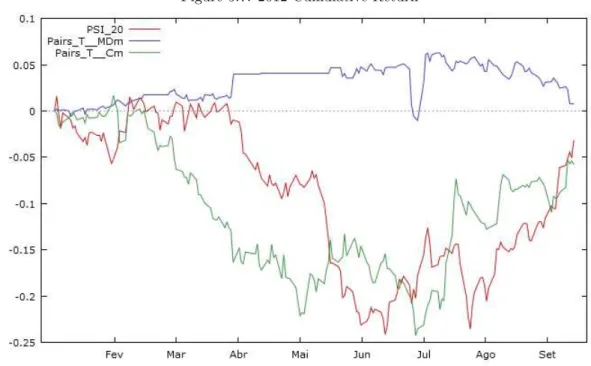
As it is possible to observe from 5.7 the behavior from the market produced a return of -3,18% in this first
9 months. This achievement was only possible by the sharp increase after August where PSI-20 raised 15%.
Observing the Pairs Trading performance on both methods, the results are not only different but also not
appealing. By the Minimum Distance method, the strategy had a stable behavior but never exceeded the
6,30% of accumulated return. The final 9 months return was of 0,81%. The Cointegration method did not
lead to a positive return. With a behaviour very similar to the market, the strategy resulted on losses of 5,77%
after the 9 months and presenting only 40% of positive daily returns. This value contrasts with the MDm,
where this value is exceeds the 65%.
Figure 5.7: 2012 Cumulative Return
Regarding 7.15 the conclusion is that in this three Quarters of 2012 the strategy was not able to beat the
market in terms of Sharpe Ratio. As it is possible to observer, the values are all very close and negative. In
terms of volatility, the Minimum Distance method produced the best outcome, presenting a volatility of 9%,
approximately half of what Cointgration method and the Market registered. Note that, May was the worst
month performance of the market (-15,19%), the second best with the Cointegration method (7,52%) and
6.
Conclusions and Implications
The present research proposes the implementation of a strategy based on quantitative analysis or statistical
arbitrage, widely know among the hedge funds and the investment banks, known as Pairs Trading. Such
proposal is applied to the Portuguese Index Market (PSI-20) and is conducted by two different approaches,
the Minimum Distance method (MDm) and the Coitegration method, in order to verify which explores better
the characteristics of the mean reversion of the pairs.
The main goal of implementing the strategy is to compare both the performance of of Pairs Trading against
the PSI-20 return and add more information about the efficiency of the Market. Although those two points are
the major objectives, there are also presented in this research additional information about the characteristics
of the strategy. For this purpose there are realised an analysis considering different values for the trigger
parameterd and also two different variants for assessing the Pairs Trading performance.
The first notorious conclusion is that for both methods the strategy outperformed the Market achieving an
annual return of 10,91% and 13,26%, with the MDm and Cointegration method respectively, versus the -0,88%
achieved by the Market. Overall, for the respective analysis period, the MDm ended the year of 2011 with
a total return of about 98% which is very close to the 106% obtained with the Cointegration method. This
outstanding performances are more notorious when compared to the total return of -15% accomplished by the
Market.
The MDm performance proved to be non related to the Markets, presenting a zeroβby rejecting the null
hypothesis which means that Pairs Trading may be called a Market Neutral strategy. In this analysis stage it
is also relevant to refer that the strategy achieved an alpha, this is, an excess return of the strategy regarding
the return of the market, of about 11% a year, which indicates that the investment annual return exceeded
that from investments with a similar risk. Here it is possible to conclude that the EMH is violated since that in
order to be considered an weak-form efficient market, the expect value of alpha, in this type o strategy, should
be zero. The Sharpe Ratio, excess return of a strategy by one unit of risk, was considerable higher than that
of Portuguese Market, Psi-20, obtaining a value of 1,43 (MDm) versus 0,09, respectively.
On the other hand, the Cointegration method, presented aβstatistically significant, equal to 0,135. This
results imply that by elaborating the Pairs Trading strategy, in the Portuguese Market, with such approach,
ultimately, the strategy can not be defined as a Market Neutral Strategy. Although this major difference from
the result obtained with the MDm, the alpha presented a value of 12,5%, supporting once again the idea that
the market present inefficiencies on its weak-form. In terms of risk-adjusted return, the Cointegration method
From the analysis of the value of the trigger rule, the results were consistent with the literature concluding
as the most profitable ad equal to 2 standard deviations. When assessing the performance of Pairs Trading strategy, it is possible to conclude that the results that were obtained were not due to an issue of luck but else
to the proficiency of the strategy.
When analysing the first 9 months of 2012 it is possible to conclude that the Minimum Distance method
is, in fact, the best approach to conduct Pairs Trading strategy. The fact that 65% of the daily returns
were positive and in the Cointegration method there was only 40%, indicates that in times of crisis the mean
reversion was not profitable because the stationary does not persist.
Another conclusion that is possible to retrieve is that in trouble times the financial markets tend to become
more efficient. In this case,and based on the MDm, both 23% of the days had not recorded any transaction
and also 9 out of the 14 stocks did not traded in the all period. This last statement indicates that there was
not any inefficiency that could be seized by Pairs Trading.
The overall results confirms both that: it is possible to achieve excess returns by using past information; that
there is still space for profiting by using trading strategies that are able to explore the market inefficiencies;
periods of crisis and low volatility tend to low the strategy’s performance; the adoption of the Minimum
Distance method turns the strategy less riskier and not that less profitable and finally; that all the variables
that were used in order to perform the strategy are, without a fact, crucial to the strategy.
It is also crucial to address one limitation of this work, that in some cases, may lead to different conclusions.
Such limitation is that the performance results are all before transaction costs. For further investigation, it
would be interesting if the Pairs Trading strategy could include accurate transactions costs. It would also be of
great interest to study the other two most cited Pairs Trading methods1 and the respectively performance and
implications to the Portuguese Index market (PSI-20). Additional, instead of defining a trigger rule, thresholds
d, it could be done by, for example, the Markov switching model or the Kalman filter. Such analysis could lead to a new path on the optimization of Pairs Trading implementation.
Bibliography
Alexander, C. and A. Dimitriu (2002). The cointegration alpha: Enhanced index tracking and long-short equity
market neutral strategies. Discussion Paper 2002-08, ISMA Centre Discussion Papers in Finance Series..
Chan, Louis K.C., J. N. and J. Lakonishok (1996). Momentum strategies. The Journal of Finance 51(5).
Cootner, P. H. (1964). The random character of stock market prices, the mit press, cambridge, massachusettes.
Coval, Joshua D., H. D. A. and T. Shumway (2005). Can individual investors beat the market? Working Paper No. 04-025.
Do, B. and R. Faff (2009). Does simple pairs trading still work? Working Paper.
Do, B. and R. Faff (2011). Are pairs trading profits robust to trading costs? Working Paper.
Elliott, Robert J., V. D. H. J. and W. P. Malcolm (2005). Pairs trading.Quantitative Finance 5(3), 271–276.
Enders, W. (1988, August). Arima and cointegration tests of ppp under fixed and flexible exchange rate
regimes. The Review of Economics and Statistics 70(3), 504–08.
Engle, R. F. and C. W. J. Granger (1987, March). Co-integration and error correction: Representation,
estimation, and testing. Econometrica 55(2), 251–76.
Fama, E. (1991, December). Efficient capital markets: Ii. Journal of Finance 46(5), 1575–617.
Fung, W. and D. Hsieh (1997). Empirical characteristics of dynamic trading strategies: the case of hedge
funds.Review of Financial Studies 10(2), 275–302.
Galenko, A., E. P. I. P. (2011). Trading in the presence of cointegration. Journal of Alternative Investments.
Gatev, E., W. N. Goetzmann, and K. G. Rouwenhorst (2006). Pairs trading: Performance of a relative-value
arbitrage rule. Review of Financial Studies 19(3), 797–827.
Jacobs, B. I. and K. N. Levy (1993). Long/short equity investing. The Journal of Portfolio Management.
Jarrow, R. (1988). Finance theory. Prentice-Hall.
Jegadeesh, N. and S. Titman (1993, March). Returns to buying winners and selling losers: Implications for
Juselius, K. and D. F. Hendry (2000, December). Explaining cointegration analysis: Part ii. Discussion Papers
00-20, University of Copenhagen. Department of Economics.
Kaan Evren Bolg¨un, E. K. and S. G¨uven (2009). Dynamic pairs trading strategy for the companies listed in
the istanbul stock exchange.Working Paper.
Khandani, A. E. and A. W. Lo (2008, November). What happened to the quants in august 2007?: Evidence
from factors and transactions data. Working Paper 14465, National Bureau of Economic Research.
Lakonishok, J., A. S. and R. W. Vishny (1994). Contrarian investment, extrapolation, and risk. The Journal of Finance 49(5), 1541–1578.
Lintner, J. (1965). The valuation of risk assets and the selection of risky investments in stock portfolios and
capital budgets. The Review of Economics and Statistics 47(1), 13–37.
Lo, A. and A. MacKinlay (1988). Stock market prices do not follow random walks: evidence from a simple
specification test. Review of Financial Studies 1(1), 41–66.
Lucas, A. (1997). Strategic and tactical asset allocation and the effect of long-run equilibrium relations. Serie
Research Memoranda 0042, VU University Amsterdam, Faculty of Economics, Business Administration and
Econometrics.
Mossin, J. (1966). Equilibrium in a capital asset market. Econometrica 34(4), 768–783.
Murray, M. P. (1994). A drunk and her dog: An illustration of cointegration and error correction. The American Statistician 48(1), 37–39.
Perlin, M. (2007, December). Evaluation of pairs trading strategy at the brazilian financial market. Journal of Derivatives & Hedge Funds 15(8308), 122–136.
Roberts, H. (1961). Market value, time, and risk.Unpublished manuscript..
Rouwenhorst, K. G. (1998). International momentum strategies. The Journal of Finance 53(1), 267–284.
Samuelson, P. A. (1965). Proof that properly anticipated prices fluctuate randomly. Industrial Management Review 6.
Sharpe, W. F. (1964). Capital asset prices: A theory of market equilibrium under conditions of risk. The Journal of Finance 19(3), 425–442.
Steve Hogan, Robert Jarrow, M. T. and M. Warachka (2004). Testing market efficiency using statistical
arbitrage with applications to momentum and value strategies. Journal of Financial Economics 73(3), 525 – 565.
Treynor, J. L. (1961). Market value, time, and risk.Unpublished manuscript..
Treynor, J. L. (1962). Toward a theory of market value of risky assets. Unpublished manuscript..
Tsay, R. S. (2005).Analysis of financial time series. Wiley.