Geosci. Model Dev., 7, 1543–1571, 2014 www.geosci-model-dev.net/7/1543/2014/ doi:10.5194/gmd-7-1543-2014
© Author(s) 2014. CC Attribution 3.0 License.
Application of a computationally efficient method to approximate
gap model results with a probabilistic approach
M. Scherstjanoi1, J. O. Kaplan2, and H. Lischke1
1Dynamic Macroecology, Landscape Dynamics, Swiss Federal Research Institute WSL, Zürcherstr. 111, 8903 Birmensdorf, Switzerland
2University of Lausanne, Géopolis, Quartier Mouline, Institute of Earth Surface Dynamics, 1015 Lausanne, Switzerland
Correspondence to:M. Scherstjanoi ([email protected])
Received: 16 January 2014 – Published in Geosci. Model Dev. Discuss.: 28 February 2014 Revised: 9 June 2014 – Accepted: 11 June 2014 – Published: 24 July 2014
Abstract. To be able to simulate climate change effects on forest dynamics over the whole of Switzerland, we adapted the second-generation DGVM (dynamic global vegetation model) LPJ-GUESS (Lund–Potsdam–Jena General Ecosys-tem Simulator) to the Alpine environment. We modified model functions, tuned model parameters, and implemented new tree species to represent the potential natural vegetation of Alpine landscapes. Furthermore, we increased the com-putational efficiency of the model to enable area-covering simulations in a fine resolution (1 km) sufficient for the com-plex topography of the Alps, which resulted in more than 32 000 simulation grid cells. To this aim, we applied the re-cently developed method GAPPARD (approximating GAP model results with a Probabilistic Approach to account for stand Replacing Disturbances) (Scherstjanoi et al., 2013) to LPJ-GUESS. GAPPARD derives mean output values from a combination of simulation runs without disturbances and a patch age distribution defined by the disturbance frequency. With this computationally efficient method, which increased the model’s speed by approximately the factor 8, we were able to faster detect the shortcomings of LPJ-GUESS func-tions and parameters. We used the adapted LPJ-GUESS to-gether with GAPPARD to assess the influence of one cli-mate change scenario on dynamics of tree species compo-sition and biomass throughout the 21st century in Switzer-land. To allow for comparison with the original model, we additionally simulated forest dynamics along a north–south transect through Switzerland. The results from this transect confirmed the high value of the GAPPARD method despite some limitations towards extreme climatic events. It allowed for the first time to obtain area-wide, detailed high-resolution
LPJ-GUESS simulation results for a large part of the Alpine region.
1 Introduction
Climate change affects species composition, forest structure and biomass of forests worldwide. The appropriate modeling of forests at a large scale is important to assess their func-tions, in particular their influence on the global carbon cy-cle (Fischlin and Midgley, 2007; Purves and Pacala, 2008). This requires model functions that describe forest dynamics, particularly with respect to forest disturbances and structure-related competition (Bonan, 2008; Quillet et al., 2010).
One commonly used but simulation time-consuming way to include structural characteristics into a DGVM is the gap approach (Botkin et al., 1972; Shugart, 1984), which stochastically simulates dynamics of tree individuals or co-horts on numerous small patches, so that the mean of all stochastic replicates builds the result of one simulation step. The second-generation DGVM LPJ-GUESS (Lund– Potsdam–Jena General Ecosystem Simulator) (Smith et al., 2001; Hickler et al., 2004) combines such an approach with plant physiological functions of the LPJ-DGVM (Sitch et al., 2003). As it uses the gap approach, LPJ-GUESS is yet not computationally efficient enough to simulate forests with a fine resolution (<1 km) on a large scale (continental to global). Area-wide simulations with LPJ-GUESS typically use resolutions of 10 or 50 arcmin (Gritti et al., 2006; Koca et al., 2006; Morales et al., 2007; Wolf et al., 2008; Hickler et al., 2012) to perform simulations on subcontinental to continental scales. To more specifically analyze model func-tions of LPJ-GUESS some studies focused on simulafunc-tions on certain stands (e.g., for Switzerland Portner et al., 2010; Manusch et al., 2012; Wolf et al., 2012). However, the most recent LPJ-GUESS parameterization led to substantial dis-crepancies at a finer scale between model results and compa-rable data (Hickler et al., 2012).
We aimed to perform simulations with a 1 km resolution over the whole of Switzerland. Our decision to use Switzer-land as a study area was supported by two main arguments: first, this specific region combines altitudinal gradients with a very rugged topography and different degrees of conti-nentality and consequently contains different climate and vegetation zones. Therefore, it is a difficult test for every modeling exercise. Partly due to that, there are no dynamic area-covering climate change impact simulation studies on Swiss forests. Second, comparatively detailed climate and soil input data are available that are necessary for our mod-eling purposes. Despite the limitations at a finer scale, we chose to use LPJ-GUESS for the modeling because it con-tains detailed plant physiological functions combined with a structured vegetation and dynamics. However, recent re-sults from Scherstjanoi et al. (2013) allow us to estimate that using a 1 km resolution over the whole of Switzerland would require several months of simulation time. To en-able simulations over a large range we used a method that was lately developed by Scherstjanoi et al. (2013). With it, GAP model results are approximated with a Probabilis-tic Approach to account for stand Replacing Disturbances (GAPPARD method).
The GAPPARD method utilizes a modified version of the von Foerster equation of age-structured population dynam-ics (von Foerster, 1959). Several other approaches also used von Foerster types to approximate gap dynamics (Kohyama, 1993; Falster et al., 2010). Moorcroft et al. (2001), e.g., ap-proximated in the second-generation DGVM ED (Ecosystem Demography Model) size and age by applying a van Foer-ster type equation. In contrast to GAPPARD, this size- and
age-approximation method is applied during the simulations and for each simulation year. Hence, and also due to a lower spatial resolution in ED (Moorcroft et al., 2001), GAPPARD has most likely a higher computational efficiency. However, this increase in efficiency comes along at the cost of less pre-cision on smaller timescales.
The approximation used by the method shortens LPJ-GUESS simulations (100 stochastic replicates) by roughly a factor of 10. Therefore, the computationally efficient sim-ulations were highly advantageous and enabled us to more rapidly analyze functions of the model and more easily adapt model parameters. This is the first time that this method is used area-wide on a large scale. Hence, our first aim was to test the applicability of the GAPPARD method. As we tested LPJ-GUESS on a finer scale than typically used and applied the model to a specific region, we expected that we will have to change model parameters and adapt model func-tions. It was, thus, our second aim to control how applica-ble the latest LPJ-GUESS parameters are to model the po-tential natural vegetation (PNV) in a heterogeneous Alpine landscape and on a finer scale, and what changes have to be made due to model functions and parameters to improve re-sults. Our third aim was to use GAPPARD with the adjusted functions and parameters, and to assess (a) the usefulness of our modifications and (b) the potential influence of one cli-mate change scenario on the development of forest biomass and species composition allover Switzerland. One main issue was the response of the different tree species to warmer and drier climates and to the increase in atmospheric CO2. Ad-ditionally, we were also interested in how the results of the adjusted LPJ-GUESS differ from the results using the most recent LPJ-GUESS functions and parameters (Hickler et al., 2012).
To sum up, our main research questions are the following. – How applicable for area-wide studies over the whole of
Switzerland is the GAPPARD method?
– How valuable are the recent LPJ-GUESS parameters and functions to model the potential natural vegetation in a heterogeneous Alpine landscape, and how do model functions and parameters have to be adapted to improve results?
– Which changes of forest biomass and species com-position are projected by simulations over the whole of Switzerland using one climate change scenario and what trends do different parameters and input data indi-cate?
2 Material and methods 2.1 LPJ-GUESS
M. Scherstjanoi et al.: Application of a computationally efficient method 1545 et al., 2001; Hickler et al., 2004). It shows characteristics
from the first-generation DGVM LPJ (Sitch et al., 2003) and the individual-based (cohort-based) gap model GUESS (Smith et al., 2001). Plant physiological and biogeochemical processes are based on the formulations in the LPJ-DGVM. Plants are either simulated as tree species (Koca et al., 2006; Hickler et al., 2012) or aggregated to PFTs.
LPJ-GUESS uses a gap approach to simulate the fate of individual trees, determined by growth, stochastic establish-ment and stochastic death processes. Other stochastic ele-ments can be climatic drivers and in particular stochastically appearing small-scale stand-replacing disturbances (distur-bance stochasticity). Due to the stochasticity, individuals and vegetation biomass on each patch develop differently and simulations of many patches have to be averaged to yield the forest dynamics, requiring a lot of computational time. For gap models in general, Bugmann et al. (1996) recommended the use of 200 stochastic replicates per stand. In LPJ-GUESS, most commonly 50 or 100 of such replicates are used (as in Koca et al., 2006; Hickler et al., 2008, 2009; Miller et al., 2008; and Wramneby et al., 2008), but to save computational time the number of patches is often even smaller (e.g., 20 in Hickler et al., 2012).
2.2 GAPPARD method
The GAPPARD method (Scherstjanoi et al., 2013) is based on the idea that a forest does not necessarily have to be rep-resented by different stochastic replicates but can be cal-culated with just one undisturbed simulation, which would be much more computationally efficient. The method as-sumes that stochastically appearing small-scale disturbance events that transfer all living biomass of a stochastic repli-cate to the litter are mainly responsible for the difference between a stochastic and a deterministic model run. In LPJ-GUESS such stand-replacing disturbances occur with a con-stant probabilitypdist. The GAPPARD method furthermore assumes that the succession after a disturbance event is al-ways the same, given a constant climate. Thus, values of state variablesystarting from bare patch produced for each sim-ulation yearain an undisturbed model run and information on the patch age distribution based on pdist can be used to approximate stochastic model run results. The expectation valueY (T )ofy, which includes the effect of small-scale dis-turbances, is calculated for each yearT in a postprocessing way:
Y (T )=(1−pdist)T y(T )
+pdist T−1
X
a=1
(1−pdist)ay(a). (1)
The results of Scherstjanoi et al. (2013) showed that the other stochastic functions of LPJ-GUESS, establishment and mortality, either do not have a significant influence or their
effect is included in the GAPPARD method. Therefore, an undisturbed model run is fully deterministic.
Using just one deterministic undisturbed run leads to an extrapolation of the vegetation succession pattern from the beginning of the simulations to the whole simulation period without considering the effect of changing drivers (in LPJ-GUESS changing climate). As a solution, additional deter-ministic undisturbed simulation runs starting from different points in time (nodes) are performed. The final result is in-terpolated between these nodes. A more detailed explanation of the derivation of the method is given in Scherstjanoi et al. (2013). For our study, we used five deterministic undisturbed simulations: one starting in 1100 with a spinup up to 1900, one starting in 1950, one in 2000, one in 2050, and one in 2080. After several tests (results not shown), and due to the results of Scherstjanoi et al. (2013) we decided to use a dis-turbance frequency of 0.0154, corresponding to a return in-terval of 65 years.
Applying the GAPPARD method does not currently al-low any spatial interactions between neighboring grid cells or patch-to-patch interactions. Therefore, seed dispersal or migration functions or the spatial mass effect of LPJ-GUESS (establishment in a patch depends on other patches’ biomass in a stand) cannot be applied.
2.3 Simulation setup
We simulated forest dynamics on all cells of a 1 km grid of Switzerland where, at the moment, forests potentially could grow. Based on the Swiss soil suitability map (Frei, 1976), we excluded rocky, urban or water areas, which led to a sim-ulation setup containing 32 214 cells.
We applied climate change after the simulation year 1900. Up to 1900 we used randomly selected values of the first 30 climate data years for the model spinup. For the 1901– 1929 simulation period, we used CRU (Climate Research Unit) data downscaled to the 1 km model grid (Mitchell et al., 2004). For the 1930–2006 simulation period, we used Swiss weather station data from the Federal Office of Meteorology and Climatology MeteoSwiss interpolated to a 100 m grid by applying the Daymet method (Thornton et al., 1997). For the 2007–2100 simulation period, we used CRU climate data of one A1B climate scenario (Mitchell et al., 2004). Along with that scenario we used CO2data that reach 703 ppm (parts per million) in 2100 (IPCC, 2001, Annex II). To be able to make statements about the CO2effect, we additionally performed simulations with constant atmospheric CO2from the simula-tion year 2000 on. A visualizasimula-tion of the climate used for the simulations is given in Fig. D2 (Appendix).
Based on the Soil Suitability Map of Switzerland (Frei, 1976), we defined the required LPJ-GUESS soil parameters: usable volumetric soil water holding capacity (fraction of soil layer depth), soil thermal diffusivities at different points of water holding capacity and an empirical parameter for the percolation equation. A more detailed description is given in Appendix C2.
2.4 Model adaptation
We applied two parameter sets to our simulations, one with existing parameters and one with new ones (see Ta-ble D10 in the Appendix). For simulations with the first parameter set we used all boreal and temperate species Hickler et al. (2012) used for their simulations, as well as C3 grass and boreal evergreen shrubs. We applied the species parameters of Hickler et al. (2012) who simulated the PNV across Europe. For boreal evergreen shrubs we additionally used parameters of Wolf et al. (2008). Here we refer to this set as the standard parameter set. Considering that LPJ-GUESS was not designed for this specific region and a fine scale and based on first tests (results not shown), we expected from the results that (1) the species distribution would differ from PNV, (2) not all important tree species would be mod-eled, and (3) the occurrence of some species might end too abruptly.
We created a second parameter set to improve simula-tions of the PNV in Alpine landscapes. For this aim, we used general knowledge and different publications on PNV (Ellenberg, 1986; Brzeziecki et al., 1993; Bohn et al., 2004; Frehner et al., 2005). We did not use stand data to fine-tune LPJ-GUESS because almost all Swiss forests have been in-fluenced by forest management for a long period. To this set, to which we will refer to as the adjusted parameter set, we additionally added the three new speciesLarix decidua,
Pinus cembra andPinus mugoas described in Scherstjanoi et al. (2013). The fine-tuning of LPJ-GUESS includes a new function to describe the leaf senescence of Larix decidua. Its photosynthetic activity decreases in fall with an s-shaped curve (based on results of Migliavacca et al. (2008), see Ap-pendix A). Furthermore, we developed a modified function-ality of the plant parameter of the maximum 20-year coldest month mean temperature for establishment. This parameter is a proxy for chilling requirements for seed germination; if the 20-year coldest month mean temperature exceeds the pa-rameter’s value, establishment of boreal species is prevented (Nienstaedt, 1967, as cited in Prentice et al., 1992). Instead of allowing no establishment above this limit, we used a func-tion that decreases the amount of new saplings with an s-shaped curve. This novelty allows shade tolerant boreal trees to also grow in more temperate vegetation zones but not to such a degree that they dominate the forests (see Appendix A for details). Based on Scherstjanoi et al. (2013), we changed further parameters mainly addressing drought resistance and temperature dependencies.
Figure 1.Location of and altitude along the analyzed transect, and location of geographic terms. The transect (blue line) is placed at a longitude of 638 000 m (Swiss CH1903/lv03 coordinates). J: Jura; C: Central Plateau; P: Prealps; N: north Alps; S: south Alps; V: Valais; T: Ticino.
2.5 Simulation evaluation
M. Scherstjanoi et al.: Application of a computationally efficient method 1547 Table 1.Root Mean Square Error of the carbon mass between
LPJ-GUESS results and GAPPARD results along the mapped transect. LPJ-GUESS used 100 stochastic replicates. Values were calculated as a mean of all simulated stands in between 1901 and 2100.
Root mean square error
Boreal evergreen shrubs 0.27
Betula pubescens 0.24
Larix decidua 0.2
Picea abies 0.27
Pinus cembra 0.27
Pinus mugo 0.22
Pinus sylvestris 0.19
Abies alba 0.25
Betula pendula 0.12
Carpinus betulus 0.13
Corylus avellana 0.14
Fagus sylvatica 0.15
Fraxinus excelsior 0.15
Quercus pubescens 0.12
Quercus robur 0.13
Tilia cordata 0.13
Total carbon mass 0.08
The terms describing geographical regions mentioned in the following sections are defined in Fig. 1. Here, we describe the biomass as in kilograms per square meter (kg m−2), con-sistent with the LPJ-GUESS output variable. Assuming that carbon makes half of the wood’s total mass and a wood den-sity of 0.5 g cm−3, 1 kgC m−2 equals 40 m3 wood ha−1 or 20 t biomass ha−1.
3 Results
3.1 Simulations along the transect
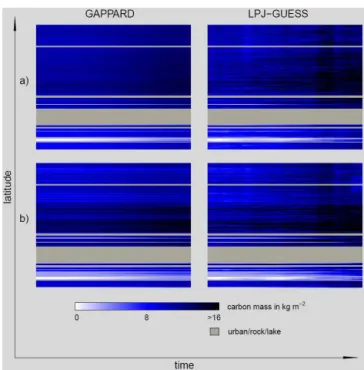
Applying the GAPPARD method generally decreased the simulation time. Simulations along the transect with LPJ-GUESS required 27 h 58 min, and thus about the 8-fold com-puting time as those with the GAPPARD method: 3 h 28 min (all values are a mean of 10 simulations). The results along the transect for both methods in general were similar (Figs. 2, 3, for the location of regions refer to Fig. 1). The RMSE for the total carbon mass between both used methods was smaller than 0.1. The RMSE for single species was always smaller than 0.3, for most species smaller than 0.2 (Table 1). Generally the GAPPARD results appear more smoothed, along the latitudinal axis as well as in time. LPJ-GUESS, on the other hand, tends to show irregularities and stripe-like patterns. Within a few years particularly the biomass of broadleaved species can decrease or increase suddenly and over large sections of the transect. However, this is the only remarkable difference between the methods.
Figure 2.Total carbon mass development along the analyzed tran-sect from 1900 (left side) to 2100 (right side) with LPJ-GUESS (100 stochastic replicates) and using the GAPPARD method.(a)adjusted parameter set;(b)standard parameter set.
Both methods used show a biomass increase of drought resistant species (e.g., Quercus pubescens and Pinus sylvestris), a shift or area extension of most species to higher altitudes, and a general increase in biomass over time. In the transect, the shift of species to higher stands can most clearly be seen in some higher elevated parts of the Valais region, where at the beginning of the 21st century no trees at all ap-peared whereas at the end of the century a high biomass of
Larix deciduaandPinus cembraoccurred. 3.2 Switzerland-wide simulations for 2000
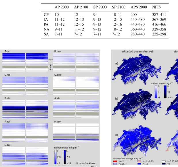
Table 2.Total simulated (rough values) and actual biomass for the years 2000 and 2100. CP: Central Plateau; JA: Jura; PA: Prealps; NA: Central, northwest and northeast Alps; SA: south, southeast and southwest Alps (see Brändli (2009) for the detailed locations of regions); SP: standard parameter set; AP: adjusted parameter set; APS: Forest stock approximated from AP 2000 results (10 kgC m−2are equivalent to 400 m3wood ha−1; see Sect. 2.5); NFIS: actual forest stock as result of the newest SWISS national forest inventory (Brändli, 2009). Units of SP and AP are in kilograms of carbon per square meter (kgC m−2). Units of APS and NFIS are in cubic meters of wood per hectare (m3wood ha−1).
AP 2000 AP 2100 SP 2000 SP 2100 APS 2000 NFIS
CP 10 12 9 10–11 400 387–411
JA 11–12 12–13 9–13 12–15 440–480 367–369
PA 11–12 12–15 9–13 12–16 440–480 416–466
NA 9–11 11–12 9–12 10–12 360–440 329–358
SA 7–11 7–12 7–11 7–12 280–440 225–298
Figure 3. Carbon mass development along the analyzed transect of nine selected species using the stochastic (100 replicates) LPJ-GUESS approach (right) and the GAPPARD method (left), both with the adjusted parameter set. The timescale on each plot extends from 1900 (left side) to 2100 (right side). A.alb:Abies alba; B.pen:
Betula pendula; F.syl:Fagus sylvatica; L.dec:Larix decidua; P.abi:
Picea abies; P.cem:Pinus cembra; P.syl:Pinus sylvestris; Q.pub:
Quercus pubescens; Q.rob:Quercus robur; 1: Central Plateau; 2:
north Alps; 3: main Alpine ridge; 4: Valais. For the location of re-gions see Fig. 1.
3.2.1 Simulations of single species for the year 2000 with the standard parameter set
Applying the standard parameter set, at the end of the 20th century either Picea abies or Fagus sylvatica dominated
Figure 4.Total carbon mass simulated with the adjusted and the standard parameter set, both using GAPPARD, for(a)2000 and(b) 2100. Total carbon mass changes between(a)and(b)are displayed in(c).
most stands (Fig. 5, for the region names cf. Fig. 1, Ta-ble 3).Fagus sylvaticagrew in stands below approximately 600 m, and was very dominant on humid sites. Up to roughly 1000 m it co-occurred withPinus sylvestrisor Picea abies
as a secondary species. Betula pendulahardly established. Most broadleaved summer-green species reached their high-est biomass values in the Central Plateau, in the dry inner Alpine valleys and valleys of the Jura.Quercus pubescens
M. Scherstjanoi et al.: Application of a computationally efficient method 1549
Figure 5.Carbon mass simulated with the standard parameter set for single species at 2000. A.alb:Abies alba; B.pen:Betula pen-dula; B. pub:Betula pubescens; F.syl:Fagus sylvatica; L.dec:Larix
decidua; P.abi: Picea abies; P.cem: Pinus cembra; P.syl: Pinus
sylvestris; Q.pub:Quercus pubescens; Q.rob:Quercus robur; BES:
boreal evergreen shrubs; OBS: other broadleaved species (Carpinus
betulus,Corylus avellana,Fraxinus excelsiorandTilia cordata).
appeared in the lowest stands of the Central Plateau. Abies albawas modeled, but did not establish at all. The occurrence ofPicea abieswas generally restricted to stands at altitudes higher than approximately 1000 m. Its dominance reached up almost to the highest potential inhabitable stands in the Alps, but a small stripe above remained where it did not establish.
Pinus sylvestris occurred only above approximately 600 m, but only established on stands belowPicea abiesor besides
Betula pubescensat the upper treeline.
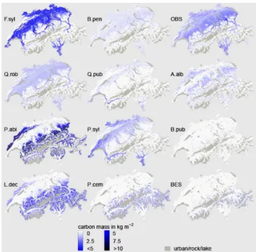
3.2.2 Simulations of single species for the year 2000 with the adjusted parameter set
Applying the adjusted parameter set generally allowed more species to co-occur and the dominance of species was less pronounced (Fig. 6, for the region names cf. Fig. 1, Table 3). In contrast to the standard parameter set, Pinus sylvestris
grew in the lower Central Plateau stands and valley bottoms of the Valais and Ticino, and was most successful on drier stands. Generally, a mixed forest that was dominated by Fa-gus sylvaticadeveloped in the Central Plateau, withQuercus roburbesidesPinus sylvestrisas the main secondary species.
Betula pendulaestablished as well on most stands below ap-proximately 1000 m but on the very dry ones, and became more successful with increasing altitude and fewer Fagus sylvatica biomass. Also, Quercus pubescens established in
Figure 6.Carbon mass simulated with the adjusted parameter set for single species at 2000. See Fig. 5 for species abbreviations.
small densities at the lowest elevation sites of the Central Plateau; it was more successful in the southwest and espe-cially in the Valais, similarly to the standard set. All the species that grew in the Central Plateau also established in the low Alpine valleys, butFagus sylvaticaandBetula pen-duladid not grow there on drier sites.Abies albaestablished, in contrast to the standard parameter set simulations. It ap-peared in the transition zone between the Central Plateau and higher altitudes, and there co-occurred with Central Plateau species orPicea abies. It did not grow in the lower parts of the Central Plateau, but increased its biomass stepwise from approximately 600 m on and decreased again at approx-imately 1200 m.Picea abieswas less dominant in the Jura and the Prealps than with the standard parameter set. Sim-ilarly toAbies alba, the biomass of Picea abies decreased gradually to zero from mountainous stands down to higher sites of the Central Plateau. Two of the three newly parame-terized species appeared as main species:Larix deciduawith gradually increasing biomass from the lower montane veg-etation zone up to the subalpine zone andPinus cembra re-stricted to the subalpine zone.
Table 3.Simulation results of selected species for the different regions. Units in kgC m−2. I: standard parameter set results for 2000; II: adjusted parameter set results for 2000; III: development of standard parameter set results until 2100; IV: development of adjusted parameter set results until 2100; a: Central Plateau and low sites in the Ticino; b: Alpine valley bottoms (submontane/colline); c: lower montane vegetation zone of Jura, Prealps and Alps; d: upper montane vegetation zone; e: subalpine vegetation zones; n.i.: not implemented; –: species did not establish or only had a very small biomass; N: none if too dry; *: strongly increases with water availability; **: strongly decreases with water availability; U: on upper stands; L: on lower stands; D: on dry sites; T: only Ticino; SA: south Alps;⇑: increase higher than 3 kgC m−2;↑: increase of 1–2 kgC m−2;ր: increase lower than 1 kgC m−2;→: roughly constant;ց: decrease lower than 1 kgC m−2;↓: decrease of 1–2 kgC m−2; : varies strongly; see Fig. 5 for species abbreviations.
F.syl B.pen Q.rob Q.pub P.syl A.alb P.abi B.pub BES L.dec P.cem
I a 6..9L,2U <0..2 0..4 2 >4..5U – – – – n.i. n.i.
b 0..6∗ <0..2 0..6 >0..5∗∗ – – – – – n.i. n.i.
c – – – – – – 5..>10 <1∗ – n.i. n.i.
d – – – – 0–10 – 1..>10* 0..5∗ – n.i. n.i.
e – – – – – – – 0..5∗ 1..4 n.i. n.i.
II a 4..6 0..3∗ 2 0.. >0..5∗∗ 2..3U – – – – –
b 5N 0..1∗ 2 1..5∗∗ >0..6∗∗ 2U – – – – –
c – – – – – 2 >0..10 <0.5∗ – 2..3 –
d – – – – – – 5..10 <0.5∗ – 4..6 –
e – – – – – – – <0.5∗ 1..4U 4..6 5
III a ցL⇑U → ցրT ⇑L↑U ցU – – – – n.i. n.i.
b ցL⇑U → ց → ցU – – – – n.i. n.i.
c րL → րN – – ց → – n.i. n.i.
d – րL րSA – – ⇑ ց – n.i. n.i.
e – – – – – – ↑ ր ցLրU n.i. n.i.
IV a ցL ցT,D ցDրU ↑Lր ↑LրU → – – – – –
b → → ցDրU ր րLցU → – – – – –
c րL ր ր – – → ց → – ց –
d – ր – – – – ↑ → – → –
e – – – – – – ⇑L ր ցLրU ⇑ ցLրU
of 1–2 kgC m−2 (Table 2). The increase was highest at the upper treeline. In the east of the Jura, most lower stands of the Valais, and in the southwest of Switzerland the increase in carbon mass was lower than 1 kgC m−2. Using the standard parameter set yielded a very similar picture. One difference is that in the Central Plateau the increase was rather small (<1 kgC m−2). Another difference is that forest biomass de-creased in lower parts east of the Jura, and in stands at the val-ley bottoms of the Ticino and the Valais (up to 1 kgC m−2).
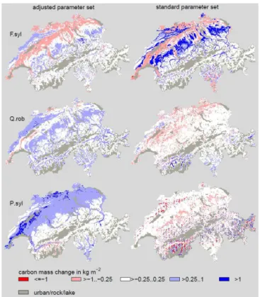
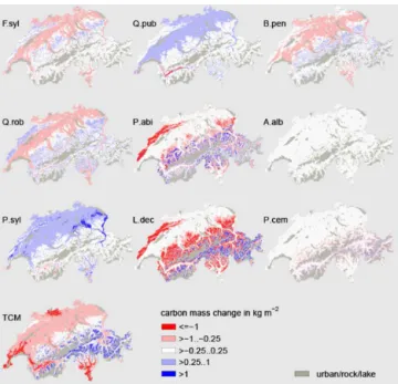
The changes in biomass show that drought-adapted species benefited most from climate change, and that bo-real species lost the most biomass in lower stands and ex-perienced a gain of biomass in higher stands (Figs. 7, 8 left; Table 3; Fig. D3 in the Appendix). Climate change led to an increase of Pinus sylvestrisbiomass in most stands. On sites in southwest and north Switzerland, and on stands of the dry inner Alpine valleys, the increase was highest. Its biomass only decreased on mid-altitudinal sites in the Valais. The biomass of Fagus sylvaticaincreased on stands of the Jura and the Prealps and decreased in the lower part of the Central Plateau.Quercus roburbiomass increased on most stands, but some low sites in the southwest. Quercus
pubescens increased its biomass on most stands and, be-sidesPinus sylvestris, was the only species benefiting from climate change in the lower part of the Central Plateau. It was also the species with the highest increase in distribution area and it only lost biomass in some stands of the south-west.Picea abiesbiomass decreased in most parts of the Jura and the Prealps. In contrast, on most stands of the Alps and higher stands of the Prealps the biomass ofPicea abies in-creased.Abies albabiomass did not change significantly. Be-sidesPicea abies, the newly implemented speciesLarix de-ciduaandPinus cembrawere most successful establishing at higher altitudes, specifically where they were not growing at the end of the 20th century. However,Larix deciduabiomass decreased in the Jura and the Prealps, andPinus cembralost approximately a third of its biomass on lower sites and only increased on very high sites.Betula pendulabenefited from the decrease inLarix deciduabiomass in the Prealps and the Jura and increased its biomass there.
M. Scherstjanoi et al.: Application of a computationally efficient method 1551
Figure 7. Changes in carbon mass between 2000 and 2100 for six selected species simulated with the adjusted parameter set. See Fig. 5 for species abbreviations.
with the standard set, this is mainly true forPinus sylvestris,
Fagus sylvatica and Quercus robur. In contrast to the ad-justed set,Pinus sylvestrislost biomass on all but a few high elevation stands and mid-altitudinal stands of the Valais, Fa-gus sylvaticaincreased its biomass largely in the higher el-evations of the Central Plateau, and the biomass ofQuercus roburdecreased on most stands of the Central Plateau. 3.4 Development under constant CO2conditions
Applying constant CO2from 2000 on led to a decrease of to-tal biomass on most stands (Fig. 9). The toto-tal carbon mass in the Central Plateau decreased by more than 2 kgC m−2. We simulated an increase of biomass only above approximately 1000 m. The only species that still benefited from the temper-ature increase in the Central Plateau wereQuercus pubescens
andPinus sylvestris.
3.5 Summary of the most important changes by adjusting the parameters
By using the adjusted parameter set we significantly changed simulation results of forest dynamics. The implementation of the three species Larix decidua, Pinus cembra and Pi-nus mugo was one major change. The modeling of partic-ularly Larix deciduaandPinus cembraand the adjustment of temperature- and drought-related parameters of species in general led to an altered species distribution in comparison to
Figure 8.Changes in carbon mass between 2000 and 2100 for three selected species compared between simulations with the adjusted parameter set and the standard parameter set. See Fig. 5 for species abbreviations.
simulations with LPJ-GUESS standard parameters. Concern-ing LPJ-GUESS standard species, we replaced especially the regions wherePinus sylvestrisandAbies albaoccurred. Moreover, we reduced the dominance ofFagus sylvaticaand
Picea abies. Furthermore, we enabled more gradual transi-tions between species of different vegetation zones, in par-ticular between Picea abies,Abies albaand species below the upper montane vegetation zone.
4 Discussion
4.1 The GAPPARD method
By applying the GAPPARD method we were able to simulate forest dynamics across Switzerland on a fine grid requiring a short simulation time. Hence, we were able to analyze the effects of the chosen climate change scenario on forest dy-namics in the heterogeneous topography of Switzerland.
Figure 9.Changes in carbon mass between 2000 and 2100 simu-lated with the adjusted parameter set under a constant CO2level from year 2000 on. See Fig. 5 for species abbreviations. TCM: total carbon mass change. Compare to Figs. 7 and 8 for single species results under a rising CO2level, and to Fig. 4 for total carbon mass results under a rising CO2level.
set and to improve functions of the complex forest model LPJ-GUESS. For the first time, simulations of LPJ-GUESS could be run over the whole of Switzerland and on all po-tentially suitable cells on a 1 km grid (more than 32 000 grid cells). Hence, the method has the potential to be applied to other regions with a similar or larger number of grid cells. The usefulness of the GAPPARD method can be highlighted even more by extrapolating the simulation time the stochastic LPJ-GUESS required for the transect (131 grid cells) across all of Switzerland (assuming that the transect is represen-tative for Switzerland). If ten processors are used in par-allel the Switzerland-wide simulations would roughly last 30 days, which complicates an analysis of results, whereas with GAPPARD Switzerland-wide simulations required only 3–4 days.
By applying GAPPARD, we indirectly showed that the parameter of LPJ-GUESS with the strongest influence on the stochasticity of results is the return interval for stand-replacing disturbances. The great influence of this parame-ter was already shown in other studies (Hickler et al., 2004; Gritti et al., 2006; Scherstjanoi et al., 2013). One great advan-tage of the GAPPARD method is that the results of the de-terministic runs, starting from different nodes (see Sect. 2.2), can easily be used for multiple values of disturbance inter-vals. The main reason for this is that GAPPARD is applied in a postprocessing way, and requires substantially less compu-tational time than the deterministic simulation runs (roughly
15 min for the whole of Switzerland). Thus, furthermore un-derlining the great potential of our method, disturbance inter-vals could also be easily implemented as stand specific (e.g., soil, management or altitude specific). However, in this study we did not focus on the analysis of disturbance frequency and chose one constant value for the disturbance interval. In con-trast to the standard LPJ-GUESS value of 100 years we used an interval of 65 years. Our decision for a low disturbance return interval was mainly based on the idea to also consider the effects of other disturbances (e.g., wind, fire, parasites, human disturbances) and was also supported by recent re-sults of Scherstjanoi et al. (2013).
The most remarkable difference in our results between the stochastic LPJ-GUESS simulations and the GAPPARD method concerns the intensity with which the biomass can change over time. Most likely, extreme climatic events, i.e., dry periods combined with high temperatures, led to ex-tinction events when simulated with the stochastic LPJ-GUESS. In a similar way the vegetation increased as a re-sponse to good growing conditions. In contrast, applying the GAPPARD method on LPJ-GUESS led to smoothed results. On the one hand this is limiting the use of the GAPPARD method on shorter temporal scales. On the other hand, the long-term trends of both methods used were very similar, and the longer temporal scale applicability is not negatively influ-enced.
Still, there are some limitations. One shortcoming of the GAPPARD method is the current impossibility of allow-ing spatial interactions (see Sect. 2.2). Especially migra-tion might have a significant influence on the change of species composition under a changing climate (Lischke, 2005; Neilson et al., 2005; Lischke et al., 2006; Epstein et al., 2007; Snell et al., 2014). The shift of species towards higher altitudes simulated here was not constrained by tree disper-sal. Whenever climatic conditions allowed, tree species grew there. Therefore, the simulated shifts might be too fast and the species composition could be biased. However, this lim-itation also addresses LPJ-GUESS as it does not include a migration function. Furthermore, the role of demographic stochasticity (stochastic establishment and mortality) has not been fully covered by the GAPPARD method, as we assume that small-scale disturbances have the biggest potential to achieve deviations from the deterministic LPJ-GUESS run. When applying the method to other models it should be first tested how much influence a demographic stochasticity has.
4.2 Switzerland-wide simulations
M. Scherstjanoi et al.: Application of a computationally efficient method 1553 e.g., of the InfoFlora (National Swiss Data and Information
Center of the Swiss Flora, http://www.infoflora.ch, last ac-cess: 8 June 2014) or of National Forest Inventory (NFI) data (Brändli, 2009), because (a) the current forest composition is biased by management, such as favoring certain species (e.g.,
Picea abies) by selective thinning and planting, and (b) it would be challenging to extrapolate the plot-based NFI data in space. Furthermore, the existing LPJ-GUESS parameteri-zation is according to a PNV. Hence, a comparison to actual forest dynamics would require taking into account manage-ment effects and would most likely cause additional changes to the LPJ-GUESS parameterization (e.g., reduced sensitiv-ity of seedlings to chilling if trees are planted, i.e., surpass the seedling stage).
4.2.1 Situation for the simulation year 2000
The total biomass we modeled in general is slightly higher than the actual forest biomass. In Table 2 our results are compared with data from the Swiss NFI (Brändli, 2009). Our simulated total biomass for the Central Plateau is closest to the NFI data, whereas the results for the Jura and Alps dif-fer more strongly from each other. Our total biomass results are also consistent with results of Erb (2004), who reported a PNV carbon mass of 12.4 kgC m−2for Austrian forests. Fur-thermore, in a study where LPJ-GUESS was used locally for a valley in the Swiss Prealps, Gimmi et al. (2009) also con-cluded that the actual biomass was slightly smaller than the assumed natural forest biomass.
Simulations with the standard parameter set led to a species distribution that revealed that the parameterization was not specifically designed for the Alpine region. It might work better on larger scales (see also Hickler et al., 2012). For the specific climate, soil properties, terrain and present species this parameterization is not adapted enough. Im-portant species were missing and the distribution of major species was not realistic. Using the standard parameter set, the spatial distribution ofPicea abiesends too abruptly at al-titudes of approximately 1000 m. Here, it should build mixed forests withAbies alba(Brzeziecki et al., 1993; Bohn et al., 2004; Frehner et al., 2005). However,Abies albadid not es-tablish at all. The most likely reason for its absence might be the combination of a low parameter value for the maxi-mum 20-year coldest month mean temperature for establish-ment (high temperatures prevent establishestablish-ment) and a high value of minimum growing degree day sum on 5◦C base
(GDDmin, high temperatures are required for establishment; columns “tc_max_e” and “gdd5min” in Table D10 in the Ap-pendix). With the standard parameter set,Pinus sylvestris ap-peared at the upper treeline. In contrast, according to PNV it is supposed to grow in the dry Alpine valleys (Bohn et al., 2004), andLarix deciduaandPinus cembraare the species that build up the upper treeline. In northern Europe, Pinus sylvestrisreaches up to the northern treeline (e.g., Kullman, 2007). However, the distribution of Pinus sylvestrisin the
Alps must be regarded separately from the one in northern Europe. The Scandinavian northern and Alpine upper tree-lines differ in terms of solar energy, angle of insolation, alti-tude, summer temperatures, wind magnialti-tude, soil properties and the biota, which might have an influence on the species composition. Due to our information onPinus sylvestrisin the Alps we changed its parameters for our study. We par-ticularly removed the limit for the maximum 20-year cold-est month mean temperature for cold-establishment so that the species can also grow in the valleys (column “tc_max_e” in Table D10 in the Appendix). To force the growth ofPinus sylvestris, especially in the Alpine valleys, additional func-tions would have to be implemented into the model. Another parameter we changed forPinus sylvestriswas GDDmin. We raised it from 500 to 600 to prevent growth at higher altitudes (column “gdd5min” in Table D10 in the Appendix). Gener-ally, information onPinus sylvestrisGDDminin the literature reaches from 500 to 950 (Mikola, 1993; Rehfeldt et al., 2003; Matías and Jump, 2012). Considering a PNV,Fagus sylvat-icais the dominant species in the Central Plateau (Brzeziecki et al., 1993; Bohn et al., 2004; Frehner et al., 2005), but it is not exactly clear what grade of dominance is most realistic. There should be at least 50 %Fagus sylvaticabiomass but in most cases less than 10 % of the biomass are of secondary tree species (Bohn et al., 2004). We decreased the drought tolerance ofFagus sylvatica(column “d_tol” in Table D10 in the Appendix). As a result, it is less abundant but still makes up approximately half of the forest biomass in the Central Plateau. With the standard parameterization set this value is higher but the species is too successful in dry regions where it should not appear under natural conditions (e.g., the east of the Valais). Another shortcoming of the standard parameter set is the low biomass ofBetula pendula. We fixed that with the adjusted parameter set when we decreased the species’ needed growing degree sum required for full leaf cover (col-umn “phenramp” in Table D10 in the Appendix) to account for its comparatively fast budburst (Murray et al., 1989). The implementation of the new species was successful. The upper treeline composition withLarix deciduaandPinus cembraas main species, and the gradual downslope decrease ofLarix decidua, is consistent to the expected distribution (Frehner et al., 2005).
4.2.2 Development in the 21st century
The total biomass increase of 1–2 kgC m−2 (equivalent to 40–80 m3 wood ha−1, see Sect. 2.5) is mainly CO
2 driven, as simulations with a constant atmospheric CO2 show (see Fig. 9). An increase of temperature alone might have the effect of making more stands potentially habitable to more species but it also increases the evapotranspiration and thus the risk of water stress situations.
strengthens this statement. Using the adjusted parameter set, the biomass of Pinus sylvestris andQuercus robur widely increased throughout the 21st century. In contrast, using the standard set their biomass in general decreased. A likely rea-son for this is a strong increase inFagus sylvaticabiomass, favored by its unrealistically high drought tolerance, espe-cially on sites initially populated byPinus sylvestris (com-pare in Fig. 8 F.syl, right, with Fig. 5 P.syl). However, also with the adjusted parameter set, Pinus sylvestrisfirst expe-rienced a decrease starting in the first half of the 20th cen-tury (Fig. 3). It is not completely clear what triggered this decrease but it could be of complex origin. Most likely slight changes in the species composition play a role, since climatic events alone can be excluded because other less drought- or cold-resistant species were not affected. Nevertheless, in the second half of the 21st century a strong increase of Pinus sylvestrisbiomass occurred, yielding a positive increment for the whole simulation period. Interestingly, Pinus sylvestris
is also one of the few species that increases its biomass on most stands even under a constant atmospheric CO2. Based on simulations with the LPJ-DGVM (same plant physiolog-ical functions as in LPJ-GUESS), Cheaib et al. (2012) re-ported a different result. They found thatPinus sylvestrisin contrast to deciduous broadleaved trees benefits less from an increase in atmospheric CO2. However, our results show that statements of a general model behavior are critical when pa-rameters are sensitive to small changes, and once more em-phasize the importance of the species composition.
We most likely overestimated the increase in biomass for species establishing in new regions, because their future dis-tribution will depend on migration rates, which we did not implement into the models used. This is in particular true for
Quercus pubescens, which established on regions very dis-tant to its origin (Fig. 3).
5 Conclusions and outlook
The results of our simulations can be regarded as a suc-cess towards (1) applying the GAPPARD method on a large scale, (2) advancing the complex forest model LPJ-GUESS,
and (3) gaining insight into forest changes as a consequence of climate change. We were able to show that GAPPARD incorporates a computationally efficient method to analyze forest dynamics on large scales. Therefore, it represents a substantial advancement in forest modeling. The GAPPARD method could potentially be applied to every gap model that uses patch replacing disturbances. Thereby simulation time would decrease, and thus the potential simulation range can increase. Furthermore, it could be applied to other types of models to include the effect of stand-replacing small-scale disturbances.
One big future task is to find a way to allow spatial interconnectivity. In particular, it should be considered to find a way to include migration functions to improve the GAPPARD method. Moreover, it could further advance the method if the effect of disturbances that are not stand-replacing will be implemented. To solve these issues and test the general applicability of GAPPARD, in the near future the method could be applied to other gap models, for example ForMind (Köhler and Huth, 1998). Furthermore, regional- to large-scale intercomparisons with the forest landscape model TreeMig (Lischke et al., 2006) are planned.
To further improve the applicability of LPJ-GUESS in Alpine landscapes, the newly found parameters and functions must be applied to different regions. It is furthermore relevant whether the new parameters and functions can also be ap-plied on a larger scale and on regions with different climates. Such studies could also go hand in hand with analyses of the influence of different disturbance regimes on the modeling of forest dynamics, since the effect of different disturbance intervals can easily be applied.
M. Scherstjanoi et al.: Application of a computationally efficient method 1555 Appendix A: New plant physiological functions
and parameters
Based on Scherstjanoi et al. (2013) we included the three new tree species: Larix decidua, Pinus cembra and Pinus mugo. Existing functions of LPJ-GUESS were applied to bothPinusspecies. However, first plausibility tests showed that these functions were not sufficient for Larix decidua, mainly due to the tree species’ specific phenology. In LPJ-GUESS, the foliage of summer-green species is transferred to the litter all at once on 1 simulation day (typically in fall) when the maximum number of equivalent days with full leaf cover per growing season exceeds a certain value. For most species, this approximation has no significant negative in-fluence because photosynthetic efficiency in general is re-duced more suddenly. However, especially for larches, leaf senescence can be a process that lasts for months during which photosynthetic intensity is reduced stepwise. Based on Migliavacca et al. (2008), Scherstjanoi et al. (2013) in-cluded this physiological trait by defining a new phenology type for Larix decidua. The tree species is modeled like a summer-green species, but in autumn the phenological state of the larches will decrease with an s-shaped curve. Here, we improved this function to make it more applicable for more varying climate conditions. For means of simplification, we decided to define a time point in a year when the process of leaf senescence will be completed, independently of climate conditions. This is also in accordance with the findings of Migliavacca et al. (2008), who reported that Larix decidua
trees of different stands complete leaf senescence roughly at the same time, independently of the senescence curve. We decided to use 1 December as that day. We then calculated the phenology ofLarix deciduadepending on the number of days since the start of fall of leavestlsand the length of the period between the start of fall of leaves and 1 Decemberdls:
phen(t ) = 1
1+0.5e
13.5
dlstls−6.75
, (A1)
so that phen (t) is close to 1 when the ratio of tls to dls is approaching 0, and close to 0 when the ratio is close to 1.
According to Scherstjanoi et al. (2013), we definedLarix deciduaas a shade-intolerant species with a high ratio of leaf area to sapwood cross-sectional area (Oren et al., 1995). The parameters of the newPinusspecies are mainly based on Pi-nus sylvestrisparameters. However, both newPinusspecies are more cold resistant, have seeds that are less drought re-sistant and their needles have a higher longevity. Moreover,
Pinus mugowas defined as shade intolerant.
In the establishment function, we changed the functional-ity of the LPJ-GUESS parameter of maximum 20-year cold-est month mean temperature for cold-establishment (tc_max_e), which prevents certain boreal species from growing in tem-perate stands. Instead of this threshold function used so far, for lowest mean monthly temperatures for the last 20 years (mt_minin Celsius degrees) above tc_max_e, saplings now
can establish. Their numbernthen decreases according to an s-shaped curve:
n = n0
1+0.5e(tc_max_f(mt_min−tc_max_e)−4.5), (A2)
with tc_max_f being a newly introduced plant-specific shape parameter that influences how intense the reduction of sapling establishment is (Table D10), and n0 being the number of saplings that establish when mt_min is below tc_max_e.
A summary of all parameters used is given in Tables D8– D10.
Appendix B: Calculation of the root mean square error The differences in carbon mass of one species between the two model outputs (Cm1,Cm2) are added up for each year (y) between 1901 and 2100. These, for each year calculated differences:
cmd,y= Cm1,y−Cm2,y, (B1)
are scaled by the mean maximum carbon mass appearing in the period defined by the time window:
cmm=max Cm1,1901, Cm2,1901, Cm1,1902, Cm2,1902, . . .,
Cm1,2100, Cm2,2100. (B2)
Then its square is added up and divided by the number of years in which the species had a positive biomass in either of both models (ycount); and the root of it is the root mean square error: RMSE= v u u u t yend P
y=ystart
C md,y Cmm 2 ycount . (B3)
Appendix C: LPJ-GUESS input data C1 Cloud coverage
In LPJ-GUESS, either daily cloud coverage or total net radia-tion is needed as an input to calculate the net primary carbon uptake. No data in the wanted resolution were available to us on either of them. However, upscaled radiation data are often not correlated to precipitation data, so that unrealistic input is produced (e.g., precipitation without cloud coverage). One possibility would have been to apply advanced geostatistical methods for the interpolation of the precipitation and net ra-diation between climate stations.
lookup tables. We discretized six cloud coverage classes to be predicted and applied three discretized explanatory variables: precipitation in a day, season and altitude. For each combi-nation of explanatory variables (5 precipitation classes×5 altitudinal classes×4 seasons) we calculated probabilities of each of the six cloud coverage classes derived from the weather station data frequency and thus created the lookup tables (Tables D2–D6). During the simulation, one cloud coverage class for a simulation day was picked depending on the three explanatory variables. If, for example, no cloud cover for a certain day is predicted with a probability of 25%, the lowest cloud coverage class will be taken if a random number between 0 and 1 is smaller than 0.25. After the cloud coverage class has been determined, the value is sampled ran-domly between the border values of the class.
C2 Soil data
M. Scherstjanoi et al.: Application of a computationally efficient method 1557 Appendix D: Tables and figures
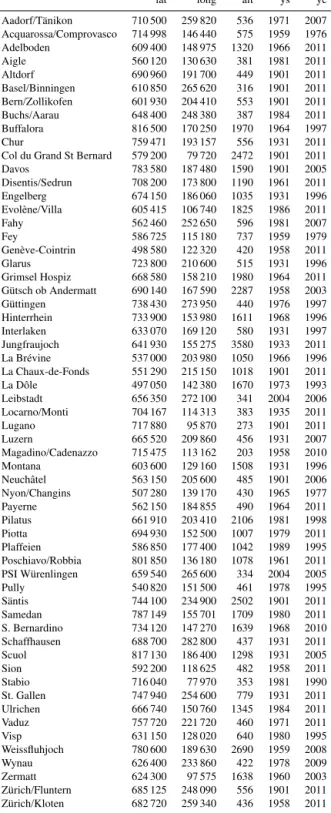
Table D1.Climate station data used to estimate cloud coverage. lat and long: latitude and longitude in meters, CH1903/lv03 (Swiss) coordi-nates; alt: altitude above sea level in meters; ys: first year of cloud coverage recording; ye: last year of cloud coverage recording. When cloud coverage was recorded at a station, precipitation was also recorded.
lat long alt ys ye
Table D2.Probabilities of cloud coverage classes for a 24 h precipitation sum of 0 cm depending on explanatory variables following selected Swiss climate weather stations. A: altitude of the climate stations; S: season; wi: winter (before day 46 or after day 319 of a year); sp: spring (between days 46 and 136 of a year); su: summer (between days 137 and 227 of a year); fa: fall (between days 228 and 318 of a year); I–IV: cloud coverage classes; I: 0 %; II: 0–20 %; III: 20–40 %; IV: 40–60 %; V: 60–80 %; VI: 80–100 % cloud coverage.
A S I II III IV V VI
<500 m wi 0.0816 0.1248 0.1367 0.1434 0.1634 0.3501 sp 0.0676 0.1646 0.1870 0.2000 0.1977 0.1830 su 0.0393 0.2196 0.2653 0.2285 0.1672 0.0802 fa 0.0555 0.1591 0.2092 0.2139 0.1847 0.1775
500– wi 0.0782 0.1089 0.1413 0.1567 0.1864 0.3285
<1000 m sp 0.0688 0.1568 0.1777 0.1979 0.2142 0.1846 su 0.0409 0.2194 0.2487 0.2288 0.1741 0.0880 fa 0.0587 0.1560 0.2055 0.2147 0.1979 0.1672
1000– wi 0.2423 0.1816 0.1872 0.1576 0.1222 0.1091
<1500 m sp 0.1146 0.1630 0.1956 0.1949 0.1815 0.1503 su 0.0395 0.1821 0.2745 0.2423 0.1805 0.0812 fa 0.1107 0.1968 0.2325 0.2004 0.1594 0.1002
1500– wi 0.2494 0.2080 0.1897 0.1496 0.1237 0.0796
<2000 km sp 0.1229 0.1717 0.1926 0.1904 0.1826 0.1397 su 0.0449 0.1816 0.2727 0.2489 0.1772 0.0747 fa 0.1270 0.1964 0.2271 0.2109 0.1559 0.0827
>= 2000 m wi 0.1958 0.2911 0.1946 0.1495 0.1030 0.0660 sp 0.1003 0.2178 0.1984 0.1849 0.1705 0.1280 su 0.0373 0.1874 0.2444 0.2435 0.1795 0.1079 fa 0.0888 0.2206 0.2300 0.2114 0.1591 0.0901
Table D3.Probabilities of cloud coverage classes for a 24 h precipitation sum of>0–4 cm depending on explanatory variables following selected Swiss climate stations. For further description see Table D2.
A S I II III IV V VI
<500 m Wi 0.0012 0.0054 0.0281 0.0815 0.2068 0.6770 Sp 0.0003 0.0047 0.0305 0.1095 0.2653 0.5897 Su 0.0014 0.0141 0.0785 0.1946 0.3245 0.3869 Fa 0.0037 0.0126 0.0566 0.1473 0.2922 0.4875
500– Wi 0.0004 0.0032 0.0255 0.0876 0.2235 0.6598
<1000 m Sp 0.0002 0.0036 0.0246 0.1034 0.2696 0.5986 Su 0.0002 0.0114 0.0685 0.1859 0.3366 0.3974 Fa 0.0015 0.0104 0.0459 0.1421 0.3135 0.4866
1000– Wi 0.0061 0.0139 0.0527 0.1199 0.2406 0.5668
<1500 m Sp 0.0012 0.0062 0.0396 0.1157 0.2541 0.5832 Su 0.0016 0.0117 0.0697 0.1974 0.3214 0.3983 Fa 0.0027 0.0143 0.0629 0.1627 0.2812 0.4761
1500– Wi 0.0060 0.0165 0.0598 0.1420 0.2636 0.5121
<2000 m Sp 0.0018 0.0109 0.0406 0.1168 0.2477 0.5821 Su 0.0006 0.0122 0.0749 0.2051 0.3207 0.3865 Fa 0.0019 0.0169 0.0602 0.1631 0.3015 0.4564
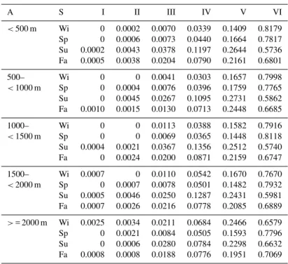
M. Scherstjanoi et al.: Application of a computationally efficient method 1559 Table D4.Probabilities of cloud coverage classes for a 24 h precipitation sum of>4–10 cm depending on explanatory variables following selected Swiss climate stations. For further description see Table D2.
A S I II III IV V VI
<500 m Wi 0 0.0002 0.0070 0.0339 0.1409 0.8179 Sp 0 0.0006 0.0073 0.0440 0.1664 0.7817 Su 0.0002 0.0043 0.0378 0.1197 0.2644 0.5736 Fa 0.0005 0.0038 0.0204 0.0790 0.2161 0.6801
500– Wi 0 0 0.0041 0.0303 0.1657 0.7998
<1000 m Sp 0 0.0004 0.0076 0.0396 0.1759 0.7765 Su 0 0.0045 0.0267 0.1095 0.2731 0.5862 Fa 0.0010 0.0015 0.0130 0.0713 0.2448 0.6685
1000– Wi 0 0 0.0113 0.0388 0.1582 0.7916
<1500 m Sp 0 0 0.0069 0.0365 0.1448 0.8118 Su 0.0004 0.0021 0.0367 0.1356 0.2512 0.5740 Fa 0 0.0024 0.0200 0.0871 0.2159 0.6747
1500– Wi 0.0007 0 0.0110 0.0542 0.1670 0.7670
<2000 m Sp 0 0.0007 0.0078 0.0501 0.1482 0.7932 Su 0.0005 0.0046 0.0250 0.1287 0.2431 0.5981 Fa 0.0007 0.0026 0.0216 0.0778 0.2085 0.6889
>= 2000 m Wi 0.0025 0.0034 0.0211 0.0684 0.2466 0.6579 Sp 0 0.0021 0.0084 0.0505 0.1593 0.7796 Su 0 0.0006 0.0280 0.0784 0.2298 0.6632 Fa 0.0008 0.0008 0.0188 0.0776 0.1951 0.7069
Table D5.Probabilities of cloud coverage classes for a 24 h precipitation sum of>10–20 cm depending on explanatory variables following selected Swiss climate stations. For further description see Table D2.
A S I II III IV V VI
<500 m Wi 0 0.0002 0.0070 0.0339 0.1409 0.8179 Sp 0 0.0006 0.0073 0.0440 0.1664 0.7817 Su 0.0002 0.0043 0.0378 0.1197 0.2644 0.5736 Fa 0.0005 0.0038 0.0204 0.0790 0.2161 0.6801
500– Wi 0 0 0.0041 0.0303 0.1657 0.7998
<1000 m Sp 0 0.0004 0.0076 0.0396 0.1759 0.7765 Su 0 0.0045 0.0267 0.1095 0.2731 0.5862 Fa 0.0010 0.0015 0.0130 0.0713 0.2448 0.6685
1000– Wi 0 0 0.0113 0.0388 0.1582 0.7916
<1500 m Sp 0 0 0.0069 0.0365 0.1448 0.8118 Su 0.0004 0.0021 0.0367 0.1356 0.2512 0.5740 Fa 0 0.0024 0.0200 0.0871 0.2159 0.6747
1500– Wi 0.0007 0 0.0110 0.0542 0.1670 0.7670
<2000 m Sp 0 0.0007 0.0078 0.0501 0.1482 0.7932 Su 0.0005 0.0046 0.0250 0.1287 0.2431 0.5981 Fa 0.0007 0.0026 0.0216 0.0778 0.2085 0.6889
Table D6.Probabilities of cloud coverage classes for a 24 h precipitation sum of>20 cm depending on explanatory variables following selected Swiss climate stations. For further description see Table D2.
A S I II III IV V VI
<500 m Wi 0 0 0 0.0019 0.0393 0.9588
Sp 0 0 0.0008 0.0068 0.0462 0.9462
Su 0 0.0004 0.0198 0.0757 0.1713 0.7327 Fa 0 0.0005 0.0097 0.0353 0.1078 0.8468
500– Wi 0 0 0 0.0024 0.0217 0.9759
<1000 m Sp 0 0 0.0045 0.0135 0.0655 0.9165 Su 0 0.0020 0.0153 0.0675 0.1554 0.7597
Fa 0 0 0.0075 0.0313 0.1314 0.8298
1000– Wi 0 0 0 0.0035 0.0318 0.9647
<1500 m Sp 0 0 0 0.0069 0.0466 0.9465
Su 0 0 0.0181 0.0683 0.1215 0.7922
Fa 0 0 0.0031 0.0251 0.0868 0.8849
1500– Wi 0 0 0 0.0014 0.0360 0.9626
<2000 m Sp 0 0 0 0.0061 0.0167 0.9772
Su 0 0 0.0060 0.0518 0.0976 0.8446
Fa 0 0 0.0011 0.0139 0.0622 0.9227
>= 2000 m Wi 0 0 0.0018 0.0062 0.0677 0.9244
Sp 0 0 0.0010 0.0089 0.0546 0.9355
Su 0 0 0.0041 0.0386 0.1269 0.8305
Fa 0 0 0.0057 0.0149 0.0744 0.9050
Table D7.Soil classification. sc: LPJ-GUESS soil code; ep: empirical parameter in percolation equation (mm day−1); vw: volumetric water holding capacity (WHC) at field capacity minus WHC at wilting point, as fraction of soil layer depth; t1–t3: thermal diffusivities (TD; in mm2s−1); t1: TD at wilting point (0 % WHC); t2: TD at 15 % WHC; t3: TD at field capacity (100 % WHC). Thermal diffusivities follow van Duin (1963) and Jury et al. (1991, Fig. 5.11.); un: unit number in soil suitability map.
sc ep vw t1 t2 t3 un
1 5.0 0.110 0.2 0.800 0.4 B3, E3, L1, P1, P4, P7, Q2, Q5, R2, R5, S1, S5, S7, T1, T3, U1, U2, U3, U5, U7, V1, V2, V3, V4, V5, V6, V7, V8, W1, W2, W3, W5, W7, W8, Y2, Y5, Z2
2 4.0 0.150 0.2 0.650 0.4 A7, A8, A9, B7, C3, C6, H1, O2, Q1
3 3.0 0.120 0.2 0.500 0.4 A1, A3, B1, C5, C7, C8, D1, E2, E4, E5, E7, F3
4 4.5 0.130 0.2 0.725 0.4 F2, F4, G1, G2, H3, H7, J2, K3, L2, L3, L4, M1, M3, N1, N3, P8, R1, R4, S2, S3, S4, S6, S8, T2, T4, U4, U6, U8, W4, W6, X2, Y1, Y4, Z3, Z4 5 4.0 0.115 0.2 0.650 0.4 B6, C2, E1, E6, E8
6 3.5 0.135 0.2 0.575 0.4 A4, A5, B2, B4, B5, B8, B9, C1, C4, D2, G3, G4, H2, H4, H5, H6, J1, K1, K2, K4, M2, M4, N2, N4, O1, O3, O4, O5, P2, P3, P5, P6, Q4, R3 X1, Y3, Z1, Z5
7 4.0 0.127 0.2 0.650 0.4 A6, E9, F1
8 9.0 0.300 0.1 0.100 0.1 Q3
M. Scherstjanoi et al.: Application of a computationally efficient method 1561 Table D8.Shade tolerance parameters. The affiliations to species are given in Table D10. st: shade tolerant; ns: nearly shade tolerant; ist: intermediate shade tolerant; si: shade intolerant; siBES: shade-intolerant boreal evergreen shrubs.
st ns ist si siBES
Minimum forest-floor PAR 1.25 1.625 2 2.5 1.5
for establishment (MJ m−2day−1)
Growth efficiency threshold 0.04 0.06 0.08 0.1 0.04 (kgC m−2year−1)
Maximum establishment rate 0.05 0.075 0.1 0.2 0.625 (saplings m−2year−1)
Recruitment shape parameter 2 4 6 10 10
after Fulton (1991)
Annual sapwood to heartwood 0.05 0.0575 0.065 0.08 0.0125 turnover rate (year−1)
Table D9.Climatic range parameters. The affiliations to species are shown in Table D10.
Boreal Temperate
Optimal temperature range 10 to 25 15 to 25 for photosynthesis (◦C)
Table D10.Specific tree parameters of I the standard and II the adjusted parameter set. One entry per species and parameter means the same parameters were used for both sets or that the species was not included in the standard parameter set (newly added species). * newly added species; ** direct comparison between I and II not meaningful because different establishment functions were used; n.i.: parameter not implemented. b: boreal; t: temperate; st: shade tolerant; ns: nearly shade tolerant; ist: intermediate shade tolerant; si: shade intolerant; e: evergreen; s: summer-green; d: summer-green with decelerated senescence; cl.range: climatic range; shade tol.: shade tolerance; ph.type: phenology type; phenramp: growing degree sum on 5◦C base required for full leaf cover; k_latosa: ratio of leaf area to sapwood cross-sectional area; rootdist_u and rootdist_l: proportion of fine roots extending into upper and lower soil layers; leaflong: leaf longevity; chill_b: changed chilling parameter (Sykes et al., 1996); d_tol: drought tolerance, lower values show higher tolerance (minimum soil water content needed for establishment, averaged over the growing season and expressed as a fraction of available water holding capacity, and water uptake efficiency); gdd5min: minimum growing degree day sum on 5◦C base, tc_max_e and tc_min_e: maximum and minimum 20-year coldest month mean temperature for establishment; tc_max_f: shape parameter for new tc_max_e function (see Appendix A); tc_min_s: maximum 20-year coldest month mean temperature for survival; k_allom2: steepness-influencing parameter in diameter to height relation; BES: boreal evergreen shrubs; B.pub:Betula pubescens; L.dec:Larix decidua; P.abi:Picea abies; P.cem:Pinus cembra; P.mug:Pinus mugo; P.syl:Pinus sylvestris; A.alb:Abies alba; B.pen:Betula pendula; C.bet:Carpinus betulus; C.ave:Corylus avellana; F.syl:Fagus sylvatica; F.exc:Fraxinus excelsior; Q.pub:Quercus pubescens; Q.rob:Quercus robur; T.cor:Tilia cordata.
BES B.pub L.dec∗ P.abi P.cem∗ P.mug∗ P.syl A.alb shade tol. I
si si si st ist si ist st
II ns
k_latosa 300 5000 5000 4000 2000 2000 2000 4000
d_tol I
0.25 0.5 0.3 0.43 0.3 0.3 0.25 0.35
II 0.38 0.33
gdd5min I
200 350 300 600 300 400 500 1450
II 600 900
tc_max_e** I
−2 – −2 −1.5 −3 −1.5 −1 −2
II −3 –
tc_max_f I n.i. n.i. n.i. n.i. n.i. n.i. n.i. n.i.
II 9 – 4.5 4.5 4.5 4.5 4.5 6
phenramp I
– 200 100 – – – – –
II 150
longevity I
50 200 500 500 500 500 500 350
II 450
k_allom2 5 40 40 40 22 30 40 40
tc_min_e – – −29 −29 −29 −29 −29 −3.5
tc_min_s – – −30 −30 −30 −30 −30 −4.5
ph.type e s d e e e e e
rootdist_u 0.8 0.8 0.6 0.8 0.6 0.6 0.6 0.8
rootdist_l 0.2 0.2 0.4 0.2 0.4 0.4 0.4 0.2
leaflong 2 0.5 0.5 4 4 4 2 4
chill_b 100 400 100 100 100 100 100 100
M. Scherstjanoi et al.: Application of a computationally efficient method 1563 Table D10.Continued.
B.pen C.bet C.ave F.syl F.exc Q.pub Q.rob T.cor
shade tol. si ist si st ist ist ist ist
k_latosa I
5000 5000 4000 5000 5000 4000 4000 5000
II 4500
d_tol I 0.42
0.33 0.3 0.3 0.4 0.2 0.25 0.33
II 0.35 0.35 0.27
gdd5min I
700 1200 800 1500 1100 1900 1100 1000
II 1300
tc_max_e – – – – – – – –
tc_max_f I n.i. n.i. n.i. n.i. n.i. n.i. n.i. n.i.
II – – – – – – – –
phenramp I 200
200 200 200 200 200 200 200
II 150
longevity 200 350 300 500 350 500 500 350
k_allom2 40 40 40 40 40 40 40 40
tc_min_e −29 −7 −10 −2.5 −15 −5 −15 −17
tc_min_s −30 −8 −11 −3.5 −16 −6 −16 −18
ph.type s s s s s s s s
phenramp 100 200 200 200 200 200 200 200
longevity 200 350 300 500 350 500 500 350
rootdist_u 0.8 0.7 0.7 0.8 0.8 0.6 0.6 0.8
rootdist_l 0.2 0.3 0.3 0.2 0.2 0.4 0.4 0.2
leaflong 0.5 0.5 0.5 0.5 0.5 0.5 0.5 0.5
chill_b 400 600 400 600 100 100 100 600
Figure D1.Soil code used in LPJ-GUESS simulations.1– urban, rocky or water areas (no forest growth);2– E: 5.0, V: 0.110, D0: 0.2, D15: 0.800, D100: 0.4;3– E: 4.0, V: 0.115, D0: 0.2, D15: 0.650, D100: 0.4;4– E: 4.0, V: 0.127, D0: 0.2, D15: 0.650, D100: 0.4;5– E: 4.5, V: 0.130, D0: 0.2, D15: 0.725, D100: 0.4;6– E: 4.0, V: 0.150, D0: 0.2, D15: 0.650, D100: 0.4;7– E: 3.5, V: 0.135, D0: 0.2, D15: 0.575, D100: 0.4;8– E: 3.0, V: 0.120, D0: 0.2, D15: 0.500, D100: 0.4;9– E: 0.2, V: 0.100, D0: 0.2, D15: 0.500, D100: 0.4,10– E: 9.0, V: 0.300, D0: 0.1, D15: 0.100, D100: 0.1. E: empirical parameter in percolation equation (k1) (mm day−1); V: volumetric water holding capacity at field capacity minus volumetric water holding capacity at wilting point, as fraction of soil layer depth; D0, D15 and D100: thermal diffusivity (mm2s−1) at 0, 15 and 100 % water holding capacity.
M. Scherstjanoi et al.: Application of a computationally efficient method 1565
Figure D3.Carbon mass simulated with the adjusted parameter set for single species at 2100. A.alb:Abies alba; B.pen:Betula pendula; B.
pub:Betula pubescens; F.syl:Fagus sylvatica; L.dec:Larix decidua; P.abi:Picea abies; P.cem:Pinus cembra; P.syl:Pinus sylvestris; Q.pub:
Quercus pubescens; Q.rob:Quercus robur; BES: boreal evergreen shrubs; OBS: other broadleaved species.
Figure D5.Carbon mass simulated with the adjusted and standard parameter set for minor species at 2000. C.bet:Carpinus betulus; C.ave:
Corylus avellana; F.exc:Fraxinus excelsior; P.mug:Pinus mugo; T.cor:Tilia cordata. Please note that a different color gradient was used
than in Fig. D3.
M. Scherstjanoi et al.: Application of a computationally efficient method 1567
Figure D7.Carbon mass development along the analyzed transect of seven selected species using the stochastic (100 stochastic replicates) LPJ-GUESS approach (right) and the GAPPARD method (left), both with the standard parameter set. The timescale in each plot extends from 1900 (left side) to 2100 (right side). See Fig. D3 for species abbreviations.