Seismic Performance Reliability of RC Structures: Application of Response Surface Method and Systemic Approach

(1)

ISSN: 2322-2093

S

eismic Performance Reliability of RC Structures: Application of

Response

Surface Method and Systemic Approach

Shahraki, H.1* and Shabakhty, N.2

1

Ph.D. Candidate, Department of Civil Engineering, Faculty of Engineering, University of Sistan and Baluchestan, Zahedan, Iran

2

Assisstant Professor, Department of Civil Engineering, Faculty of Engineering, University of Sistan and Baluchestan, Zahedan, Iran

Received: 6 Aug. 2013; Revised: 2 Mar. 2014; Accepted: 11 Mar. 2014

ABSTRACT: The present study presents an algorithm that models uncertainties at the structural component level to estimate the performance reliability of RC structures. The method calculates the performance reliability using a systemic approach and incorporates the improved response surface method based on sampling blocks using the first-order reliability method and conditional reliability indices. The results of the proposed method at different performance levels were compared to bound techniques and the overall approach. It was shown that the proposed algorithm appropriately estimates the reliability of the seismic performance of RC structures at different damage levels for the structural components. The results indicated that performance reliability indices increased when then on-performance scenarios were examined for high levels of components damage.

Keywords: RC Structures, Reliability, Response Surface Method, Seismic Performance, Systemic Approach

INTRODUCTION

Earthquakes are natural hazards that can inflict irreparable damage to civil structures and human societies. To mitigate loss from earthquakes, researchers have attempted to

forecast structural behavior during

earthquakes. Public expectation for the design of structures that perform adequately during an earthquake has increased. Since there are inherent uncertainties in ground motion intensity, material properties and external loads, a comprehensive evaluation of the seismic performance of RC structures that considers these uncertainties is necessary.

One technique for modeling

uncertainties in a structure is the Monte Carlo Simulation (MCS). Although the results of this technique are accurate, real



Corresponding author Email: shahraki.h@hotmail.com

structures require significant computational effort. Response Surface Method (RSM) is a set of mathematical and statistical techniques that have been proposed to

address this problem (Bucher and

Bourgund, 1990). In RSM, an explicit approximation is formed for the implicit

Limit State Function (LSF) using

deterministic structural analysis to calculate the reliability of a structure by the First Order Reliability Method (FORM) or Second Order Reliability Method (SORM). Bucher and Bourgund (1990) proposed a Response Surface Function (RSF) to approximate the LSF as a second order polynomial without interaction terms. They used a fitted RSF for the primary estimation of a design point and then updated the RSF using the mean vectors of the random variables and design point.

(2)

and Bourgund by updating the cycles of the RSF coefficients. They found that sampling in the tails of the distributions does not significantly improve failure probability and that the accuracy of the

approximation depends on LSF

specifications. Guan and Melchers (2001) considered a second order polynomial RSF without interaction terms and studied sensitivity to failure probability rather than position of the experimental points. Their parametric study of explicit and implicit LSF showed that the position of the experimental points significantly affected RSF approximation and the corresponding failure probability.

Kaymaz and MacMahon (2005)

proposed a weighted regression to calculate RSF parameters and calculated weights according to LSF values for experimental points. Their research indicated that this improves approximation for experimental points close to LSF. Gavin and Yau (2008) proposed higher order polynomials to approximate LSF. They considered a non-constant order polynomial for LSF and determined the order of this polynomial using statistical analysis of its coefficients. Their results indicated that the probability of failure was calculated accurately and there was no significant correlation with the size of domains of the experimental points. It should be noted that this technique may lead to ill-conditioned systems of equations. Nguyen et al. (2009) suggested an improved response surface calculated using a cumulative method. They employed a linear RSF at the first repetition, and a parabolic RSF for subsequent repetitions. They selected the experimental points using RSF partial derivatives toward random variables and RSF coefficients calculated using the weighted regression technique. Their results indicated that the algorithm improved convergence speed, and that sensitivity to the size of the experimental points decreased. Kang et al. (2010) proposed an improved response surface using moving least squares approximation

to consider higher weights for experimental points close to the design points. By using numerical examples, they showed that this technique can estimate failure probability accurately.

Vamvatsikos and Cornell (2002) and Dolsek and Fajfar (2007) proposed a probabilistic framework to relate ground motion intensity to structural response and

performance. In this method, the

displacement capacity and transition point of a structure are calculated using a set of ground motion records. The output curves indicate the cumulative probability of structural collapse in terms of ground motion intensity. Liel et al. (2009) presented these curves for flexural RC structures by contributing uncertainties in the ground motion and the modeling parameters. Buratti et al. (2010) used first- and second-order RSFs to evaluate these curves for RC structures. They considered the uncertainties of the material properties, external loads and ground motion in the RSM explicitly using random factors. They indicated that this RSF is sensitive to sampling design and the results of second-order RSF are more accurate than those of first-order RSF.

The fact that uncertainties should be incorporated at the component level of a structure to assess reliability of seismic performance has been less studied. The seismic performance reliability of a RC structure against earthquake should be evaluated by systemic analysis that includes uncertainties at the component level. The present study proposes an integrated algorithm for this purpose based on nonlinear dynamic analysis, improved

RSM, FORM, conditional reliability

indices and linear safety margins for different levels of components damage.

STRUCTURAL MODEL

(3)

calculates its maximum response. There are two categories for the nonlinear dynamic analysis of RC structures. The first is to present the overall behavior of each structural component in terms of a macro-model. The second is to discretize each structural component into smaller units and then capture the overall behavior of a component from the behavior of the smaller units (micro-models). Micro-modeling schemes are usually unsuitable

for nonlinear dynamic analysis of

structural systems because of their huge computational requirements.

An alternative model is based on fiber formulation. In a fiber model, the structural element is divided into a discrete number of segments. This model assumes constant fiber properties over each segment length based on the properties of the monitored slice at the center of each segment. The nonlinear behavior of the element is monitored in the control sections, which are in turn discretized into longitudinal fibers of plane concrete and reinforcing steel. The nonlinear behavior of the section is then captured from the integration of the nonlinear stress-strain relationship of the fibers. This feature

allows modeling of any type of RC structural element more accurately.

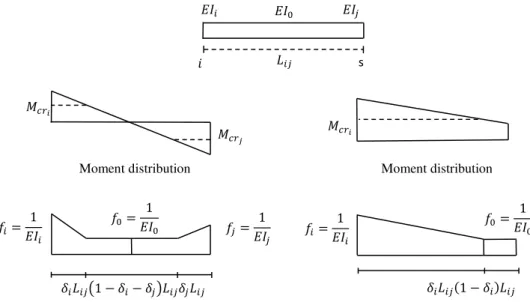
Structural members of the RC frame are subdivided into a discrete number of Sub-Elements (SEs). Flexural, shear and axial deformations are considered in the SE of the columns, although axial deformations are ignored in the SE of the beams. Flexural and shear components of the deformation are coupled in the spread plasticity formulation and the axial deformations are modeled using a linear elastic spring element. The flexibility distribution in the SE is assumed to follow the distribution shown in Figure 1, where EIi and EIj are the current flexural stiffness

of the sections at end i and j, respectively; EI0 is the elastic stiffness at the center of

the SE; i and j are the yield penetration

coefficients; Lij is the length of the SE; and

Mcr is the section cracking moment. The

yield penetration coefficients are first

calculated for the current moment

distribution, and then checked with the previous maximum penetration lengths ( imax and jmax). These coefficients cannot

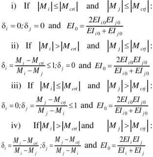
be smaller than the previous maximum values, regardless of the current moment distribution. Based on the moment distribution, four cases are considered:

Fig. 1. Spread plasticity model based on flexibility distribution in sub-element.

s

�

� = � = � =

− −

a) Flexibility distribution (single curvature) Moment distribution

�

� = � =

−

(4)

i) If Mi  Mcri and Mj Mcrj :

0 0

i ; j

    and ₀ 0 0

0 0

2 i j

i j

EI EI EI

EI EI

 _

ii) If M_i  M_cri and M_j M_crj :

1 0

i cri

i j

M M

;

M M



  _    and ₀ 0 0

0 0

2 i j

i j

EI EI EI

EI EI

 _

iii) If M_i  M_cri and M_j  M_crj :

0 j crj 1

i j

j i

M M

;

M M



    _  and 0 0 0

0 0

2 i j

i j

EI EI EI

EI EI

 _

iv) IfM_i  M_cri and M_j  M_crj :

j crj

i cri

i j

i j j i

M M

;

M M M M

 

  _   _ and ₀ 2 i j

i j

EI EI EI

EI EI

 _

where Mcri and Mcrj: are the cracking

moments of the section corresponding to the sign of the applied moments; EIi0 and

EIj0: are the elastic stiffness of the sections

at the ends of the SE. Flexural stiffness EIi

and EIj: are determined from the hysteretic

model. Special provisions are made in the model to adjust the flexibility distribution of the SE where yield penetration has taken place on the entire SE and i+ j>1.

In such cases, EI0 is modified to capture

the actual distribution considering a new

set of yield penetration coefficients that will satisfy i+ j≤1 (Valles et al., 2005).

The moment-curvature envelope

describes the changes in the force capacity

from deformation during nonlinear

analysis. In this study, the model proposed by Kunnath et al. (1992) has been used. This model is based on a tri-linear moment-curvature envelope (Figure 2) where Mcr: is the cracking moment, My is

the yield moment, Mu: is the ultimate

moment, cr is the cracking curvature, y is

the yield curvature, and u is the ultimate

curvature of the RC section.

Another aspect of nonlinear dynamic analysis is modeling the hysteretic behavior of the structural elements. The 3-parameter Park hysteretic model was used in this study. This hysteretic model incorporates stiffness degradation, strength deterioration, non-symmetric response, slip-lock, and a tri- linear monotonic envelope. It traces the hysteretic behavior of an element as it changes from one linear stage to another based upon the history of the deformations. This model is depicted schematically in Figure3; a more complete description of the hysteretic model is provided in Park et al. (1987).

Fig. 2.Moment curvature envelope for reinforced concrete sections.

�u

�y

M

Mu

My

Mcr

(5)

Fig. 3.Hysteretic model used in this study (Park et al., 1987).

Concrete material properties are defined by points in the stress-strain curve shown in Figure 4a. Five points define the stress-strain relationship under compression and one point for defines the stress-strain relationship under tension. The curve proposed by Kent and Park (1971) was adopted for concrete under compression in this study. Since confinement does not significantly affect maximum compressive stress, the model only considers the effect of confinement on the downward slope of the concrete stress-strain curve (Figure 4a).

Factor ZF defines the shape of the

descending branch, as expressed by Kent and Park (1971). The material model for the steel reinforcing bars is shown in

Figure 4b which considers the yielding of steel and strain hardening.

The moment distribution along a structural element subjected to lateral loading is linear (Figure 1a) and the presence of gravity loads will alter the distribution. The structural model takes these variations into account using several SEs at the structural members. The structure is first subjected to gravity loading, followed by dynamic analysis for ground motion. Nonlinear dynamic analysis uses a combination of the Newmark-Beta integration method and the pseudo-force method. This formulation was implemented in IDARC (Valles et al., 2005).

a) Concrete material. b) Steel material.

Fig. 4.Properties of materials (Valles et al., 2005).

� �

�

∆

�

�� = × ��

=_� .

5 + �5 ℎ− �� 5 ℎ

Confined Concrete

�

�� 5

�5 �� . ��

. ��

Unconfined Concrete

�

� = . ��

= _.�

�� _�

��

(6)

IMPROVED RSM FOR APPROXIMATING LSF

LSF is defined implicitly in real structures. RSM replaces the exact implicit LSF, g(X), with a simple and approximate one as:

g( X ) ( C ;X ) (1)

where : is the RSF, X: is the random variable vector, C: is the parameter vector of the RSF calculated by regression analysis using responses at specific data points (experimental points). Polynomials are used in structural random analysis as the RSF to provide simplicity and

continuity of random variables

(Rajashekhar and Ellingwood, 1993). The two factors that affect the accuracy are polynomial order and selection of the experimental points. The polynomial order should be a compromise between accuracy and efficiency of analysis. By focusing on accuracy, higher order polynomials can be used to acquire the LSF exactly; however,

high-order polynomials increase the

computational effort required to fit the RSF and may create an ill-conditioned system of equations (Rajashekhar and Ellingwood, 1993). Polynomial order should be selected to significantly decrease computational efforts for efficiency. In other words, using RSF with fewer parameters can decrease the number of the LSF assessments, which is important in problems with large numbers of random variables. Consequently, a second-order polynomial with interaction terms is employed in this study as:

 

2

0

1 1

1

1 1

N N

i i ii i

i i

N N

ij i j

i j i

X c c X c X

c X X

 

   

  

_



_



 

(2)

where c0, ci, cii, and c :ij are the

polynomial coefficients with numbers

1 1 2

2

N ( N )

N 

  and X ;ii  1, , N :are the

random variables. The polynomial

coefficients are calculated using a set of experimental points on the exact LSF. Since selection of these experimental points is required to estimate LSF accurately, an iterative scheme is applied to fit the RSF appropriately.

At the first iteration, experimental points with numbers 10×[1+2N+N(N-1)/2)] are generated around the means of the random variables. The responses of the structure are calculated using nonlinear dynamic analysis at the experimental points and RSF is fitted as Eq. (2).

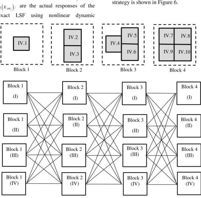
Using the RSF and FORM, the reliability index, corresponding design point, and the relative importance of the random variables are acquired. Identifying the relative importance of the random variables is accomplished using the importance measures of FORM (Der Kiureghian, 2004). The sampling blocks are based on the relative importance of random variables and, in next iterations, the new experimental points are generated in the sampling blocks. The experimental points are: (i) ascending, (ii) descending, (iii) maximum in the middle and descending on the sides, and (iv) minimum in the middle and ascending on the sides of each block.

(7)

improved linear interpolation strategy is used (Huh and Haldar, 2002) as:

   





1

if DP j C j

C j

C j C j DP j C j

C j DP j

g X g X :

g( X )

X X X X

g( X ) g( X )





   _ (3a)

   





1

if _{DP j} _{C j}

CDP j

C j DP j C j DP j

DP j C j

g X g X :

g( X )

X X X X

g( X ) g( X )





   _ (3b)

where X_{C j} and X_DPj: are the coordinates of the center point and the design point for iteration j, respectively; g( X_{C j}) and

 

DPj

g X : are the actual responses of the

exact LSF using nonlinear dynamic

analysis at X_{C j} and X_DPj :, respectively; and

1

C j

X _ : is the new center point for the

next iteration. This iterative scheme will

continue until it converges at

predetermined tolerance criteria. The convergence criteria are considered to be

1 0 05

C_j C_j C_j

( X _ X ) / X  . , and

1 1 0 01

DP_j DP_j DP_j

( X X _ ) / X _  . . In the final iteration, information on the most recent center is used to estimate the final RSF. FORM is then applied to calculate the reliability index and the coordinates of the most probable failure point. The graphical representation of the proposed strategy is shown in Figure 6.

Fig. 5. The block sampling design based on relative importance of random variables. Block 4

(IV) Block 4

(III) Block 4

(II) Block 4

(I)

Block 1 (II)

Block 1 (III)

Block 1 (IV)

IV.1

Block 1

IV.2

IV.3

Block 2

IV.4

IV.5

IV.6

Block 3

IV.7 IV.8

IV.9 IV.10

Block 4

Block 1 (I)

Block 2 (I)

Block 2 (II)

Block 2 (III)

Block 2 (IV)

Block 3 (I)

Block 3 (II)

Block 3 (III)

(8)

Fig. 6.Flowchart of the proposed algorithm for fitting LSF and calculating performance reliability indices.

Unsatisfied: Intermediate iteration

Convergence check

ییاهن رارکت : یلب

No

Yes Final iteration

Start

� → �

Generate experimental points

NLDA

Estimate responses at all experimental points

FORM

Calculate � _� and relative importance of random

variables

Apply the linear interpolation

Find � ₊₁

Calculate �, � _�

End No

First iteration Yes

Creating the sampling blocks

Determine unknown coefficients of RSF

(9)

The quality and accuracy of RSF at each iteration is checked using the descriptive statistical measure, �_�� , which

shows the correlation between the

estimated and exact values of LSF (Nguyen et al., 2009):





2 2 1 2

1

adj

R R R

o 





  

 (4)

 



 



 

2

2 2

1 1

2 1

;

o k o k k

k k

o _k

k

R

g X g X C X

g X



 



  _  _ 

   

 

 



(5)

where O: is the number of experimental

points, and v: is the number of RSF

parameters. 2

adj

R value close to 1 is

indicative of the accuracy of the RSF. If this criterion is less than 0.9, the quality of RSF should be increased (Liel et al.,

2009). The criterion 2

0.95

adj

R  has been

used in this study.

SYSTEMIC APPROACH FOR

PERFORMANCE RELIABILITY

ANALYSIS

In reliability analysis of structures, failure by a LSF is denoted as g: →R where : is the n-dimensional basic variable space. If



1, 2, , n



Z  Z Z Z is the vector of standard

normal variables with joint probability density function n,g should be defined such

that the space can be divided into failure domain  _f





. The

failure probability of P_f can defined as:

 



0



 

f

f n

P P g Z z dz





  

_

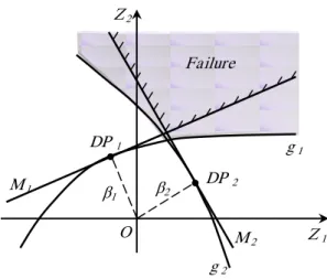
₍₆₎

If g in a point called “design point” is linearized in distance β from the origin of coordinates (Figure7), Pf can be estimated

as:

 

   

1 1 1 1

0

f n n

n n

P P Z Z

P Z Z

  

   

    

      (7)

where 



1,,n



: is the vector of the

directional cosines of linearized LSF, �: is the Hasofer-Lind reliability index (1974) and Φ: is the standard normal cumulative distribution function. It can be said that:

1 1 n n

M Z  Z  (8)

is the linearized safety margin of a structure.

Fig. 7. Reliability analysis for two structural elements with linear safety margins.

DP 2

DP 1

β1 β2

O _M

2

M 1

g 2

g 1

Z 1

Z 2

(10)

Since a real structure contains many components, a systemic approach should be applied to calculate its reliability index. In the systemic approach, the structure can be modeled as a series system, a parallel system, or combination of these. In a series system with m elements (Figure8), the safety margins of the elements are:

 

; 1, 2, ,

i i

M g X i  m ₍₉₎

where X 



X1, ,Xn



: is the vector of basic

variables, g ii



1,2, , m



: is the nonlinear

LSF. Using Z T X

 

, basic variables can transform into standard normal variables so that the failure probability of element i can be calculated as:

 



 



 







1





 



0 0

fi i i

i i

P P M P g X

P g T Z P h Z

    

   (10)

By linearizing hiat the design point, Pfi

can be estimated as:

 









  0 0 Φ fi i T

i i i

P P h Z

P  Z  

  

    (11)

where : is the unit normal vector in the design point.

Fig. 8.Series and parallel systems of structural elements.

By returning to the series system in Figure 8, the probability of failure of this system can be calculated as (Hohenbichler and Rackwitz, 1983):

 













1 1 1 0 0

1 1 Φ ;

m fs i i m T i i i m T

i i m

i

P P g X

P Z P Z             _  _      _   _         _  _  _ _     (12)

where 



1,,m



, ij : 

 

   is the correlation coefficient matrix for the linearized safety margins, and Φ :m is the

multi-normal distribution function. Failure probability for a parallel system with m elements (Figure8) can be estimated using the same method (Hohenbichler and Rackwitz, 1983):  













1 1 1 0 0 Φ ; m fP i i m T i i i m T

i i m

i

P P g X

P Z P Z              _  _      _   _        _  _ _ _     (13)

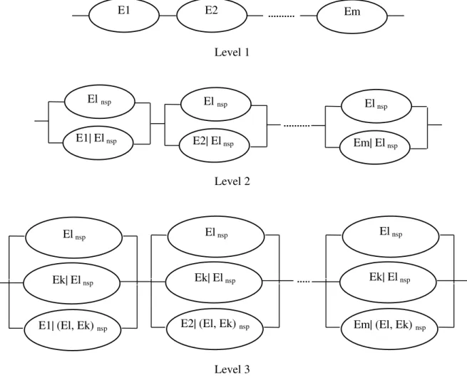
Different performance scenarios for the structural components are essential to estimate the performance reliability of a structure. In this study, a systematic approach is proposed which is general in concept to allow use for different levels of component damage. In this approach, the performance reliability index of the structural system at level 0 is calculated based on a single element as:

0 min 1, , i sys i m   

  (14)

E1 E2 Em

(11)

At level 0, each component is

considered separately from other

components and interactions between components are ignored in the reliability analysis. This provides a very optimistic estimation of performance reliability.

At level 1, performance reliability index of the structure was estimated using a series system of structural components, as shown in Figure 9. Since calculation of the multi-normal distribution function in Eq. (12) is not possible for a large number of

components, the non-performance

probability of the structure can be estimated using components of this series system (Thoft-Christensen and Sørensen, 1984). Based on the β values of these components in



min,min 1



, min: is the

smallest reliability index, and ₁:is the

defined positive value, are selected. The components are called critical components. Performance reliability at level 2 is estimated using a series system in which the components are parallel subsystems (critical pairs), as shown in Figure 9. At level 2, it is assumed that component l with the smallest reliability index, does not satisfy the specific performance level. New reliability

indices for all components (except

component l) are calculated and the

smallest value of β is considered to be min.

Components with a conditional reliability index in interval



min,min 2



(where

2:



 is a positive value) are combined as parallel by component l. Consequently, the performance reliability of structural system at level 2 can be estimated as follows:

Fig. 9. Modeling of the performance reliability of structural system at level 1 to level 3.

E1 E2 Em

Level 1

El nsp

E1| El nsp

El nsp

E2| El nsp

El nsp

Em| El nsp

Level 2

El nsp

Ek| El nsp

E1| (El, Ek) nsp

El nsp

Ek| El nsp

E2| (El, Ek) nsp

El nsp

Ek| El nsp

Em| (El, Ek) nsp

(12)

i) Calculate the conditional reliability indexes for all components except l.

ii) Evaluate the linearized safety margin for components in



min,min 2



.

iii) Estimate the non-performance probability and the equivalent linearized safety margin for parallel subsystems.

iv) Assess correlation between parallel subsystems.

v) Calculate the non-performance probability of the series system.

At level 2, safety margin Ml for

component l and conditional safety margin

nsp Ei|El

M for component i are calculated.

Subscript nsp indicates that the specific performance level has not been satisfied. Using correlation coefficients El , Ei El| nsp

and reliability indices El and Ei El| _nsp , the

non-performance probability of this

parallel subsystem (Pnpp) is calculated as:





2 | , |

Φ , ;

nsp nsp

npp El Ei El El Ei El

P     ₍₁₅₎

This method is repeated for all critical pairs of elements. A linear safety margin

 

p

M is then estimated for each parallel

subsystem and the performance reliability index of the series system consisting of the parallel subsystems is calculated. MEi El| nsp

and Mp: are computed where reliability index e: is equal to Ei El| nsp and p,

meaning they have similar sensitivity to variations in the basic variables. In this study, equivalent linear safety margin

 

e

M is considered as (Gollwitzer and

Rackwitz, 1983):

1 1

1

e e e e

k n

n

e e

j j

j

M Z Z

Z           



(16)

where



1, ,



:

e e e

n

    is a unit vector

calculated with a slight increase (� ̅ in basic variables using a numerical derivative:

0 2 0 1 | 0 | 2 0 1 | or [ | ] |

; 1, ,

[ | ] nsp nsp p e o o n p j j Ei El o

n Ei El

j j o n                           _{ }  



(17)

System reliability at level 3 is estimated based on critical triples of components. At level 3, the critical component pair l and k is identified as having the smallest reliability indices of all elements. It is assumed that the specific performance level is not satisfied for components l and k. New reliability indices are calculated for all

components (except l and k) where the

smallest value of β is _min. Components in the range of [min,min 3] (where 3: is

a positive value) are combined with

components l and k to form parallel

subsystems, as shown in Figure9. When the performance reliability of a structural system is accomplished at level 3, safety

margin _ , _

nsp El Ek

M for components l and k,

and safety margin |_ , _

nsp Ei El Ek

M for component

i are calculated. Using these safety margins, reliability indices  El, Ek El| nsp and Ei El Ek| , _nsp

and correlation matrix ρ, the

non-performance probability for the parallel subsystems can be estimated as:





3 | |( , )

Φ , , ;

nsp nsp

npp El Ek El Ei El Ek

P      (18)

The equivalent linear safety margins

 

e

M are then calculated for critical triples

of components and the performance reliability of the structure at level 3 is estimated using a series system that includes the parallel subsystems. The performance reliability of the structure can be estimated using this algorithm at level

3

(13)

correlate, only one is selected in the proposed algorithm.

NUMERICAL CASE STUDY AND DISCUSSION

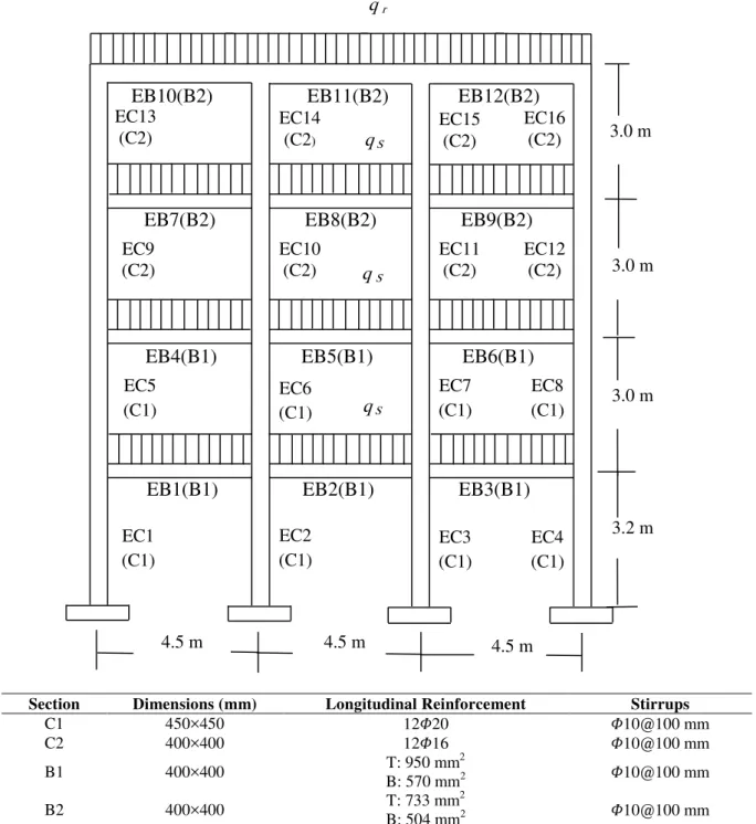
The seismic performance reliability of a RC frame structure (Figure 10) is evaluated in this section. The target structure was part of a residential building

located in a zone of very high seismic hazard that was designed according to Iranian standard 2800 and the Iranian

concrete code. The basic variables

affecting seismic performance were: i) Ground motion intensity. ii) Gravity loads.

iii) Material properties

Section Dimensions (mm) Longitudinal Reinforcement Stirrups

C1 450×450 12�20 �10@100 mm

C2 400×400 12�16 �10@100 mm

B1 400×400 T: 950 mm

2

B: 570 mm2 �10@100 mm

B2 400×400 T: 733 mm

2

B: 504 mm2 �10@100 mm

Fig. 10. The RC moment frame structure. EB10(B2) EB11(B2) EB12(B2)

EB7(B2) EB8(B2) EB9(B2)

4.5 m 4.5 m _{4.5 m}

3.2 m 3.0 m 3.0 m 3.0 m

EC1 (C1)

q S

q r

EB1(B1) EB2(B1) EB3(B1)

EC2 (C1)

EC3 (C1)

EC4 (C1)

EB4(B1) EB5(B1) EB6(B1)

EC5 (C1)

EC6 (C1)

EC7 (C1)

EC8 (C1) EC9

(C2)

EC10 (C2)

EC11 (C2)

EC12 (C2) EC13

(C2)

EC14 (C2)

EC15 (C2)

(14)

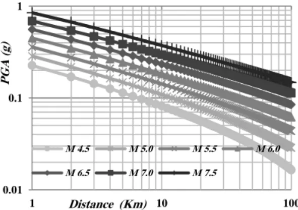
A variety of ground-motion intensity measures are available. In this study, Peak Ground Acceleration (PGA) was selected because it correlates strongly with the performance variables of interest, such as the damage index or inter-story drift (Vamvatsikos and Cornell, 2002; Dolsek and Fajfar, 2007). Hazard information is available for this parameter on the probability of an earthquake of a given intensity measure. Other uncertainties are implicitly incorporated using the model proposed by Khademi (2004). Figure 11 shows this model for soil type I in Iranian standard 2800. The values for the Khademi model were assessed using the chi-squared test for the PGA distribution. An extreme type II (Frechet) distribution gave the best

approximation of PGA. The cumulative

density function of this distribution is:

  exp( ) k

A

u

F a

a



 

 _ _

  (19)

where k=2.31 is the shape parameter and u= 0.133 is the scale parameter. The

probability density function of this

distribution is shown in Figure 12. Based on

this model and three assumptions for a magnitude equal to 7.0, an epicenter distance of 9 km, and soil type I from

Iranian standard 2800, the PGA was

calculated to be 0.35g. This value has a 10% probability of being exceeded in 50 years, giving mean and standard deviations

of this variable of 0.21g and 0.29g,

respectively. The Tabas time

history (Tabas Station, 1978; Figure 13) was used for nonlinear dynamic analysis. It has a significant duration of 16.21 s, which is greater than the 10 s and 3T = 1.38s values recommended in Iranian standard 2800.

Fig. 11.PGA variations for different magnitudes based on Khademi model (Khademi, 2004).

Fig. 12.Probability density function of PGA. 0.01

0.1 1

1 10 100

PGA

(

g

)

Distance (Km)

M 4.5 M 5.0 M 5.5 M 6.0

M 6.5 M 7.0 M 7.5

Histogram Frechet

PGA (g)

0.9 0.8

0.7 0.6

0.5 0.4

0.3 0.2 0.1

0.36

0.32

0.28

0.24

0.2

0.16

0.12

0.08

0.04

0

f

(pga

(15)

Fig. 13.Tabas earthquake time history.

Gravity loads are another source of uncertainty. Actual building details can vary from those used in the original design (for example, layers of roofing are often added during the life of a building) and unit weights are imperfect. The gravity loads of stories (qs) and roof (qr) were

considered distinctly to be a combination of dead load and 20% live load; their nominal (design) values were specified based on Section 6 of the Iranian building national regulations for a loading width of 4 m. It was assumed that the gravity loads (bias factor =1.05 and C.O.V=0.15) had a normal distribution (Table 1) (Ellingwood et al., 1980; Nowak and Collin, 2000).

Uncertainty in the force-deformation relationships of the structural elements derives from a variety of sources. Material properties differ from those assumed in the analysis, and real stress-strain behavior at the element-fiber level differs from engineering idealizations. Uncertainties in material properties should be incorporated into the performance reliability analysis of a structure. For this purpose, the compressive strength of concrete (fc),

concrete strain at compressive strength (c0), ultimate strain of concrete (cu), yield

strength of steel bars (Fsy), ultimate

strength of steel bars (Fsu), elasticity

modulus of steel bars (Es), and strain at

start of hardening of steel bars (SH) were

considered as random variables.

Ellingwood et al. (1980) and SAKO (1999) indicated that a lognormal distribution is appropriate for the parameters of concrete and reinforcing steel materials (Table 1).

Risk is always estimated based on LSFs, which can be broadly divided into serviceability and strength limit state functions. For seismic loading, the design may be controlled using the serviceability

criteria (Wen et al., 2003). LSF

corresponding to these criteria was formulated using the recommendations given in design codes. The general form of a serviceability limit state was defined as:



0 025 0 1



 

CPBE PRB PRB

g X   . , .   X (26)

-1.0 -0.8 -0.6 -0.4 -0.2 0.0 0.2 0.4 0.6 0.8 1.0

0 4 8 12 16 20 24 28 32

A

c

(

g

)

(16)

where _PRCand _PRB: are the maximum plastic rotation in column and beam elements of the structure, respectively. Threshold values of maximum plastic rotation are considered with a lognormal distribution and numbers in parentheses are means and coefficients of variation for the given performance levels (FEMA 356, 2000; ATC-40, 1996).

Table 1. Parameters of the probability distribution of random variables.

R. V. Mean S.D. Distribution Type

fc 30 MPa 4.5 MPa Lognormal

c0 2×10-3 3×10-4 Lognormal

cu 35×10-4 5.25×10-4 Lognormal

fy 400 MPa 20 MPa Lognormal

fu 600 MPa 30 MPa Lognormal

ES 2 × 105MPa 10 4MPa Lognormal

�� 3×10-2 3×10-3 Lognormal

qS 39.43 KN/m 5.92 KN/m Normal

qr 33.78 KN/m 5.07 KN/m Normal

PGA 0.21 g 0.29 g Extreme

type II

Figure 14 shows the performance reliability indices for structural elements. At performance levels IO, LS and CP, EB8 element had the smallest performance

reliability index between structural

members; accordingly, reliability of the structural system was estimated at level 0 by this component. Figure14 indicates that elements EB8, EB7, EC9, EC10, EC14, ..., EC5, and EC6 surpassed IO, LS and CP

The results of performance reliability are shown in Table 2 at level 1, where the

structural system was modeled as a series system (Figure 15). The bivariate and trivariate normal cumulative distribution functions were calculated using Drezner (1990, 1994), and the method suggested by Genz and Bretz (1999, 2002) was applied for 4 or more dimensions. Since the calculated values for the multivariate normal cumulative distribution function were accurate to  ₄, ₁ was selected such that the number of critical elements is 4. The Boole and KHD bounds (Song and Der Kiureghian, 2003) at level 1 were calculated at different performance levels. Table 2 confirmed the accuracy of the performance reliability analysis at level 1. At level 2, it was assumed that the maximum plastic rotation in EB8 exceeded threshold values IO, LS and CP, and the structural system was modeled as a series system of parallel subsystems (Figure 15). The results of performance reliability and the Boole and KHD bounds at level 2 are shown in Table 3. The performance reliability at level 3 was calculated using critical triples of the structural elements (Figure 15) and the results are shown in Table 4. The results of performance reliability analysis at level 4 are presented in Table 5. The performance reliability indices and the probabilities at different levels are compared in Figure 16, which indicates that the performance reliability indices increased from level 1 to level 4. At level 4, 3 structural components did not satisfy the specific performance level, meaning that the probability of such a scenario is less than level 1.

Table 2.The performance reliability of the RC frame structure with systemic approach at level 1.

Performance Level : IO

βmin Δβ1 Critical Elements β1 P1nsp Boole Bound KHD Bound

0.8521 0.12 EB8, EB7, EC9, EC10 0.48723 0.31305 0.19708 - 0.54664 0.24642-0.33076

Performance Level : LS

1.5560 0.146 EB8, EB7, EC9, EC10 1.47327 0.07034 0.05985 - 0.19316 0.06364-0.07267

Performance Level : CP

(17)

Fig. 14.The performance reliability indexes of Structural elements and corresponding probabilities.

Fig. 15. Performance reliability of the RC frame structure with systemic approach at level 1 to level 4.

EB8 EB7 EC6

Level 1 EB8 nsp

EB7|EB8 nsp

EB8 nsp EC9|EB8 nsp

EB8 nsp EC6|EB8 nsp Level 2

EB8 nsp

EB7|EB8 nsp

EC9| (EB8, EB7) nsp

EB8 nsp

EB7| EB8 nsp

EC10| (EB8, EB7) nsp

EB8 nsp

EB7| EB8 nsp

EC6| (EB8, EB7)nsp

Level 3

EB8 nsp

EB7| EB8 nsp

EC9| (EB8, EB7) nsp

EC10| (EB8, EB7, EC9)nsp

EB8 nsp

EB7| EB8 nsp

EC9| (EB8, EB7) nsp

EB8 nsp

EB7| EB8 nsp

EC9| (EB8, EB7) nsp

Level 4

β P

(18)

-0.52447 0.82 EB8EB7, EB8EC9,

EB8EC10, EB8EC14 0.98178 0.1631 0.1596 - 0.4543 0.16155-0.16313

-1.2553 0.82 EB8EB7, EB8EC9,

EB8EC10, EB8EC14 1.5505 0.06051 0.0585 - 0.1992 0.05973-0.06099

-1.3421 1.1 EB8EB7, EB8EC9,

EB8EC10, EB8EC14 1.6797 0.04651 0.04483 - 0.15531 0.04589-0.04655

0.86058 0.35 EB8EB7EC9, EB8EB7EC10,

EB8EB7EC14, EB8EB7EB5 1.69717 0.04483 0.04475 - 0.17859 0.04480-0.04487

1.65082 0.2 EB8EB7EC9, EB8EB7EC10,

EB8EB7EC14, EB8EB7EB5 2.3945 0.00832 0.00832 - 0.03606

0.00832-0.008323

1.8054 0.2 EB8EB7EC9, EB8EB7EC10,

EB8EB7EC14, EB8EB7EB5 2.5561 0.00529 0.00529 - 0.02254

0.00529-0.005294

0.8635 0.45

EB8EB7EC9EC14, EB8EB7EC9EC10, EB8EB7EC9EB5,

EB8EB7EC9EB4

1.8766 0.03029 0.03016-0.1132 0.03019-0.03035

1.6949 0.23

EB8EB7EC9EB4

2.5005 0.0062 0.00618-0.0264 0.0062-0.00622

1.83503 0.21

EB8EB7EC9EB4

2.6563 0.003951 0.00395-0.01631 0.003950-0.003953

To verify the results of the proposed

systemic approach, the overall

performance reliability of this structure was assessed. In the overall approach, the maximum drift and total damage index criteria (Valles et al., 2005) were applied and the LSFs have been defined as:

 



0 01 0 1

 

2 0 8 0 1

CP DI DI

(19)

β P

nsp where _MD and _DI : are the maximum

drift and total damage index, respectively. The values in parentheses are the means (FEMA 356, 2000, ATC-40, 1996, Valles et al., 2005) and coefficients of variation. Variability of the maximum drift and total damage index are shown in lognormal and beta distributions, respectively (Moller et al., 2009). Performance reliability indices of the structure were calculated for LSFs as Eqs. (27) to (31) and the results are shown in Table 6. The results were

compared with the performance reliability

indices of MCS using 105 simulations. The

results were appropriate and the relative error of the performance reliability indices (except for gIO

 

X ) were less than 0.01.

Table 6 shows that the performance thresholds based on maximum drift were more conservative than thresholds based on the damage index. The results of the overall and systemic approaches are compared in Figure 17.

Fig. 16.Performance reliability analysis of the RC frame structure with systemic approach in different levels.

Fig. 17. Comparison of the performance reliability of the RC frame structure in overall and systemic approaches.

0 0.4 0.8 1.2 1.6 2 2.4 2.8

L 0 L 1 L 2 MD DI L 3 L 4

CP

LS

IO

β _nsp

0 0.04 0.08 0.12 0.16 0.2 0.24 0.28 0.32

L 0 L 1 L 2 MD DI L 3 L 4

CP

LS

IO

(20)

Table 6. The performance reliability of the RC frame structure with overall approach.

LSF Analysis β Pnsp

gIO (X)

FORM 1.2907 0.098402

MCS 1.245 0.106484

gLS1 (X)

FORM 1.9794 0.02388

MCS 1.9765 0.02405

gLS2 (X)

FORM 2.156 0.01554

MCS 2.1425 0.01608

gCP1 (X)

FORM 2.4185 0.007792

MCS 2.4162 0.007842

gCP2 (X)

FORM 2.4974 0.006255

MCS 2.4955 0.006289

The figure indicates that the overall approach corresponded to levels 2 and 3 of the proposed systemic approach. The non-performance probabilities in the overall approach actually indicated that one structural component exceeded the given performance level in the proposed method.

CONCLUSIONS

The present paper proposes an integrated algorithm for reliability assessment of the seismic performance of RC structures. This algorithm incorporates uncertainty at the component level and is a combination of an improved RSM at the component level and a systemic approach for structural system analysis.

In the improved RSM, an iterative scheme to approximate the exact LSF is applied. In this method, structural response parameter was calculated by nonlinear dynamical analyses at the sample points. LSF was estimated using a second-order polynomial with interaction terms and

FORM was used for calculating

performance reliability index and relative importance of random variables. In the next iterations, sampling center point was updated through a linear interpolation strategy which caused LSF to be properly evaluated in the design point. The main advantage of the improved RSM is that the experimental points are generated in sampling blocks based on the importance ranking of random variables. The sampling

design generates more samples for

significant variables to allow adequate

estimate of the LSF. The sampling design decreases computational efforts and the computational time of the algorithm. The seismic performance reliability of the structural component is calculated using the final fitted RSF and FORM.

Another benefit of the proposed algorithm is that the reliability analysis of the RC structure uses a systemic approach that employs the most probable non-performance scenario at the structural component level to establish the series and parallel subsystems. This scenario consists of components with a smaller reliability index at different damage levels that are used to compute the final reliability index of the structural system.

The proposed method was used for a RC frame structure. The LSFs were defined based on the maximum plastic rotation at the structural component level. Uncertainties in the material properties and gravity loads were incorporated and earthquake uncertainty was explicitly included in the PGA, which is dependent on the magnitude, epicenter distance and type of site soil. The results showed that the non-performance probabilities of the

structure decreased when the

non-performance scenarios were formed at high levels of this algorithm.

(21)

using the general acceptance criteria of maximum story drift and global damage index. The results showed that the performance reliability indices of the overall approach corresponded to the reliability indices at interval between levels 2 to 3 for the proposed method. It should be noted that the overall approach provided seismic performance reliability only with one index, while the proposed method provided seismic performance reliability at different levels of component damage.

REFERENCES

ATC-40. (1996). Seismic Evaluation and Retrofit of

concrete Buildings, Applied Technology

Council, Redwood City, Seismic Safety Commission State of California, Report No. SSC 96-01.

Bucher, C.G. and Bourgund, U. (1990). “A fast and

efficient response surface approach for

structural reliability problems”, Structural Safety, 7(1), 57–66.

Buratti, N., Ferracuti, B. and Savoia, M. (2010). Response surface with random factors for

seismic fragility of reinforced concrete frames”,

Structural Safety, 32(1), 42-51.

Der Kiureghian, A. (2004). First- and second-order reliability methods, In Nikolaidis E., Ghiocel D. M., Singhal S., (Eds.), Engineering Design Reliability Handbook, Chapter 14, CRC Press LLC, ISBN0-8493-1180-2.

Dolsek, M. and Fajfar, P. (2007), “Simplified

probabilistic seismic performance assessment of plan-asymmetric buildings”, Earthquake

Engineering and Structural Dynamics, 36(13),

2021–2041.

Drezner, Z. (1994). “Computation of the trivariate normal integral”, Mathematics of Computation, 62(205), 289–294.

Drezner, Z. and Wesolowsky, G.O. (1990). “On the

computation of the bivariate normal integral”,

Journal of Statistical Computation and

Simulation, 35(1), 101–107.

Ellingwood, B., Galambos T.V., MacGregor J.G. and Cornell, C.A. (1980). Development of a probability based load criterion for American

national standard A58: Building code

requirements for minimum design loads in buildings and other structures, National Bureau of Standards Special Publication No. 577, Washington D.C.

FEMA. (2000). Pre-standard and commentary for seismic rehabilitation of buildings, Report No.

FEMA-356, Federal Emergency Management Agency, Washington D.C.

Gavin, H.P. and Yau, S.C. (2008). “High-order limit state functions in the response surface

method for structural reliability analysis”,

Structural Safety, 30(2), 162–179.

Genz, A. and Bretz, F. (1999). “Numerical computation of multivariate probabilities with application to power calculation of multiple

contrasts”, Journal of Statistical Computation

and Simulation, 63(4), 361–378.

Genz, A. and Bretz, F. (2002). “Comparison of

methods for the computation of multivariate probabilities", Journal of Computational and

Graphical Statistics, 11(4), 950–971.

Gollwitzer, S. and Rackwitz, R. (1983).

“Equivalent components in first-order system

reliability”, Reliability Engineering, 5(2), 99– 115.

Guan, X.L. and Melchers, R.E. (2001). ” Effect of response surface parameter variation on

structural reliability estimates”, Structural

Safety, 23(4), 429–440.

Hasofer, A.M. and Lind, N.C. (1974). “Exact and

invariant second-moment code format”, Journal of Engineering Mechanics, ASCE, 100(1), 111-121.

Hohenbichler, M. and Rackwitz, R. (1983). “First

-Order concepts in system reliability”, Structural

Safety,1(3), 177–188.

Huh, J. and Haldar, A. (2002). "Seismic reliability of nonlinear frames with PR connections using systematic RSM", Probabilistic Engineering

Mechanics, 17(2), 177–190.

Iranian Code of Concrete, (2000). 3rd Edition, Technical Office of Management and Development of Standards, Management and Planning Organization of Iran, (in Persian). Iranian Code of Practice for Seismic Resistant

Design of Buildings, (2005), Standard No. 2800, 3rdEdition, Building and Housing Research Center.

Kang, S.C., Koh, H.M. and Choo, J.F. (2010). “An

efficient response surface method using moving least squares approximation for structural

reliability analysis”, Probabilistic Engineering Mechanics, 25(4), 365-371.

Kaymaz, I. and McMahon, C.A. (2005). “A response surface method based on weighted

regression for structural reliability analysis”,

Probabilistic Engineering Mechanics, 20(1), 11–17.

Kent, D.C. and Park, R. (1971). "Flexural members with confined concrete", Journal of Structural Division, ASCE, 97(ST7), 1969-1990.

(22)

Research Report BHRC Publication No. R-376, Tehran, Iran.

Kunnath, S.K., Reinhorn, A.M. and Abel, J.F.

(1992). “A computational tool for seismic performance of reinforced concrete buildings”,

Computers and Structures, 41(1), 157-173. Liel, A.B., Haselton, C.B., Deierlein, G.G. and

Baker, W.B. (2009). “Incorporating modeling uncertainties in the assessment of seismic

collapse risk of buildings”, Structural Safety, 31(2), 197-211.

Moller, O., Foschi, R.O., Quiroz, L.M. and

Rubinstein, M. (2009). “Structural optimization

for performance-based design in earthquake

engineering: Applications of neural networks”,

Structural Safety, 31(6), 490–499.

Nguyen, X.S., Sellier, A., Duprat, F. and Pons G. (2009). “Adaptive response surface method based on a double weighted regression

technique”, Probabilistic Engineering

Mechanics, 24(2), 135–143.

Nowak, A.S. and Collins, K.R. (2000). Reliability of Structures, McGraw-Hill, New York. Park, Y.J., Reinhorn, A.M. and Kunnath, S.K.

(1987). IDARC: Inelastic Damage Analysis of Reinforced Concrete frame - shear-wall structures, Technical Report NCEER-87-0008, State University of New York at Buffalo. Rajashekhar, M.R. and Ellingwood, B.R. (1993).

“A new look at the response surface approach for reliability analysis”, Structural Safety, 12(3), 205–220.

Song, J. and Der Kiureghian, A. (2003). “Bounds

on system reliability by linear programming”,

Journal of Engineering Mechanics, 129(6), 627-636.

Thoft-Christensen, P. and Sørensen, J.D. (1984).

“Reliability analysis of elasto-plastic

structures”, Proceedings of 11th IFIP

Conferences on System Modeling and

Optimization, Copenhagen, Springer-Verlag, 556–566.

Valles, R.E., Reinhorn, A.M., Kunnath, S.K., Li, C. and Madan, A. (2005). IDARC 2D Version 6.1: A computer program for inelastic damage

analysis of buildings, Technical Report

NCEER-96-0010, State University of New York at Buffalo.