www.biogeosciences.net/14/511/2017/ doi:10.5194/bg-14-511-2017
© Author(s) 2017. CC Attribution 3.0 License.
Environmental conditions for alternative tree-cover
states in high latitudes
Beniamino Abis1,2and Victor Brovkin2
1International Max Planck Research School on Earth System Modelling, Hamburg, Germany 2The Land in the Earth System, Max Planck Institute for Meteorology, Hamburg, Germany
Correspondence to:Beniamino Abis ([email protected])
Received: 20 September 2016 – Published in Biogeosciences Discuss.: 11 October 2016 Revised: 27 December 2016 – Accepted: 4 January 2017 – Published: 2 February 2017
Abstract. Previous analysis of the vegetation cover from
remote sensing revealed the existence of three alternative modes in the frequency distribution of boreal tree cover: a sparsely vegetated treeless state, an open woodland state, and a forest state. Identifying which are the regions subject to multimodality, and assessing which are the main factors un-derlying their existence, is important to project future change of natural vegetation cover and its effect on climate.
We study the link between the tree-cover fraction distri-bution and eight globally observed environmental factors: mean annual rainfall, mean minimum temperature, growing degree days above 0◦C, permafrost distribution, mean spring soil moisture, wildfire occurrence frequency, soil texture, and mean thawing depth. Through the use of generalised addi-tive models, conditional histograms, and phase-space anal-ysis, we find that environmental conditions exert a strong control over the tree-cover distribution, uniquely determining its state among the three dominant modes in∼95 % of the
cases. Additionally, we find that the link between individual environmental variables and tree cover is different within the four boreal regions considered here, namely eastern North Eurasia, western North Eurasia, eastern North America, and western North America. Furthermore, using a classification based on rainfall, minimum temperatures, permafrost distri-bution, soil moisture, wildfire frequency, and soil texture, we show the location of areas with potentially alternative tree-cover states under the same environmental conditions in the boreal region. These areas, although encompassing a minor fraction of the boreal area (∼5 %), correspond to possible
transition zones with a reduced resilience to disturbances. Hence, they are of interest for a more detailed analysis of land–atmosphere interactions.
1 Introduction
Forest ecosystems are a fundamental component of the Earth, as they contribute to its biophysical and biogeochemical pro-cesses (Brovkin et al., 2009), and harbour a large propor-tion of global biodiversity (Crowther et al., 2015). However, changes in species composition, structure, and function are happening in several forests around the world (Phillips et al., 2009; Lindner et al., 2010; Poulter et al., 2013; Reyer et al., 2015b). These changes originate from a combination of en-vironmental changes, such as CO2 concentration, drought, and nitrogen deposition (Hyvönen et al., 2007; Michaelian et al., 2011; Brouwers et al., 2013; Brando et al., 2014; Reyer et al., 2015a), and local drivers, both anthropogenic and not, such as forest management, wildfires, and grazing (Volney and Fleming, 2000; Malhi et al., 2008; Barona et al., 2010; DeFries et al., 2010; Bond and Midgley, 2012; Bryan et al., 2013). Environmental and climate changes, as well as ex-treme events, are likely to play a more prominent role in fu-ture decades (Johnstone et al., 2010; Orlowsky and Senevi-ratne, 2012; Coumou and Rahmstorf, 2012; IPCC, 2013), af-fecting the resilience of forests – i.e. the ability to absorb disturbances maintaining similar structure and functioning (Scheffer, 2009) – and possibly pushing them towards tip-ping points and alternative tree-cover states (IPCC, 2013; Reyer et al., 2015a), potentially inducing ecosystem shifts (Scheffer, 2009).
resilience (Scheffer, 2009; Hirota et al., 2011; IPCC, 2013; Reyer et al., 2015a). To this end, in this paper, we investigate the relationship between environment and remotely sensed tree-cover distribution within the boreal ecozone. Through the use of generalised additive models (GAMs), conditional histograms, and phase-space analysis, we assess whether al-ternative stable tree-cover states are possible in the boreal forest, and under which environmental conditions, as under-standing the mechanisms underpinning them is a key point to assess future ecosystem changes (Reyer et al., 2015a).
The boreal forest is an ecosystem of key importance in the Earth system, as it encompasses almost 30 % of the global forest area and comprises about 0.74 trillion densely
dis-tributed trees (Crowther et al., 2015). Despite a low diver-sity of tree species, a boreal forest’s structure and composi-tion depend on interaccomposi-tions between several factors, includ-ing precipitation, air temperature, available solar radiation, nutrient availability, soil moisture, soil temperature, presence of permafrost, depth of forest floor organic layer, forest fires, and insect outbreaks (Kenneth Hare and Ritchie, 1972; Hein-selman, 1981; Bonan, 1989; Shugart et al., 1992; Soja et al., 2007; Gauthier et al., 2015). The boreal ecozone is highly sensitive to changes in climate and can affect the global cli-mate system through its numerous feedbacks, the most im-portant ones related to albedo changes, soil moisture recy-cling, and the carbon cycle (Bonan, 2008; Gauthier et al., 2015; Steffen et al., 2015). In fact, vegetation at high latitudes can influence albedo through its distribution and through its snow-masking effect, leading to warmer temperatures (Bo-nan et al., 1992). During winter, a snow-covered forest has a lower albedo than snow-covered low vegetation, as tall trees mask the snow on the ground (Otterman et al., 1984; Bo-nan, 2008). Additionally, differences between species distri-butions can affect albedo in summer, as dark conifers have a lower albedo than deciduous trees or shrubs (Eugster et al., 2000). On the other hand, during the growing season, trees induce a cooling effect due to enhanced evapotranspiration with respect to low vegetation (Brovkin et al., 2009). Finally, the boreal forest acts as a carbon sink (Gauthier et al., 2015) and is responsible for an estimated∼20 % of the world’s
for-est total sequfor-estered carbon (Pan et al., 2011; Gauthier et al., 2015). The balance between these effects determines how the boreal forest influences climate, which, in turn, affects vege-tation.
Despite its multiple roles in regulating climate, the dynam-ics of the boreal ecosystem regarding gradual changes and critical transitions are not yet understood (Bel et al., 2012; Scheffer et al., 2012). In this context, multimodality of the tree-cover distribution has recently been detected within the boreal biome (Scheffer et al., 2012). An analysis of the veg-etation cover from remote sensing revealed the existence of three alternative modes in the frequency distribution of bo-real trees (Scheffer et al., 2012; Xu et al., 2015): a sparsely vegetated treeless state, an open woodland “savanna”-like state, and a forest state. In particular, it has been observed
that, over a broad temperature range, these three vegetation modes coexist (Scheffer et al., 2012; Xu et al., 2015); on the other hand, areas with intermediate tree cover between these distinct modes are relatively rare, suggesting that they may represent unstable temporary states (Scheffer et al., 2012). Furthermore, it has been shown that multimodality of the tree cover does not ensue from multimodality of environmental conditions, suggesting that these three modes could represent alternative stable states acting as attractors (Scheffer et al., 2012), a stable state being the state an ecosystem will return to after any small perturbation (May, 1977). Hence, identi-fying which are the regions subject to multimodality, and as-sessing which are the main factors underlying their existence, is important both to understand boreal forest dynamics, and to project future changes of natural vegetation cover and their effect on climate.
We do acknowledge that vegetation and climatic vari-ables are linked through a more differentiated set of interac-tions than just mean annual rainfall, temperature, and forest cover. Henceforth, to improve our understanding of the bo-real ecosystem dynamics, we investigate the impact of eight globally observed environmental variables (EVs) on the tree-cover fraction (TCF) distribution. To do so, we make use of satellite products spanning the time period up until 2010, incorporating both spatial and temporal information in our analysis, and taking into account the past variability of the boreal ecosystem. Furthermore, we investigate whether the three observed vegetation modes could represent alternative stable tree-cover states. To this end, we make use of GAMs, conditional histograms, phase-space analysis, and statistical tests.
In a similar fashion, it has previously been hypothesised that tropical forests and savannas can be alternative stable states under the same environmental conditions. Evidence for bistability in the tropics has been inferred through fire exclu-sion experiments (Moreira, 2000; Higgins et al., 2007), field observations and pollen records (Warman and Moles, 2009; Favier et al., 2012; de L. Dantas et al., 2013; Fletcher et al., 2014), mathematical models (Staver and Levin, 2012; van Nes et al., 2014; Baudena et al., 2015; Staal et al., 2015), and satellite remote sensing (Hirota et al., 2011; Staver et al., 2011a, b; Yin et al., 2015).
it has been suggested that trimodality of the tree-cover dis-tribution is not necessarily due to wildfires, since it can be achieved through nonlinearities in vegetation dynamics and strong climate control (Good et al., 2016). The picture is far from complete, as there is evidence that other environmental factors might play a fundamental role in controlling the tree-cover distribution (Mills et al., 2013; Veenendaal et al., 2015; Staal and Flores, 2015; Lloyd and Veenendaal, 2016).
2 Methods and materials
2.1 Environmental variables
We study the link between the tree-cover fraction dis-tribution of eight globally observed environmental vari-ables (EVs): mean annual rainfall (MAR), mean minimum temperature (MTmin), growing degree days above 0◦C (GDD0), permafrost distribution (PZI), mean spring soil moisture (MSSM), wildfire occurrence frequency (FF), soil texture (ST), and mean thawing depth (MTD). These fac-tors are chosen based on the work of Kenneth Hare and Ritchie (1972); Woodward (1987); Bonan (1989); Bonan and Shugart (1989); Shugart et al. (1992); Kenkel et al. (1997), as they represent the main drivers of the boreal forest biome. Environmental variables can be broadly grouped into tem-perature, water availability, and disturbances factors.
Temperature factors include mean minimum temperature, growing degree days above 0◦C, permafrost distribution, and mean thawing depth. Soil and air temperature are two major factors responsible for boreal forest structure and dynamics (Kenneth Hare and Ritchie, 1972; Bonan, 1989; Havranek and Tranquillini, 1995). To survive frost and dessication, during winter, coniferous trees enter a period of dormancy, characterised by the suspension of growth processes and a reduction of metabolic activity (Havranek and Tranquillini, 1995). Hence, tree growth and expansion is only possible during extended periods with air temperature above 0◦C. We use growing degree days above 0◦C, calculated from the NCEP/NCAR reanalysis 1998–2010 (Kalnay et al., 1996), as a measure of the extent of the growing season. Growing degree days above 0◦C (◦C yr−1), in fact, measure heat ac-cumulation as the sum of the mean daily temperatures above 0◦C through a year. Furthermore, low soil and air temper-atures have several other important consequences. Cold air temperatures are the main regulator of the distribution of per-mafrost, the condition of soil when its temperature remains below 0◦C continuously for at least 2 years. Permafrost and low soil temperatures, on the other hand, impede infiltration and regulate the release of water from the seasonal melting of the active soil layer, inhibit water uptake and root elongation, restrict nutrient availability, and slow down organic matter decomposition (Woodward, 1987; Bonan, 1989). To include these effects, we use the mean minimum temperature at 2 m (◦C), and the permafrost distribution (unitless). Minimum
temperatures are obtained from the NCEP/NCAR reanaly-sis 1998–2010 (Kalnay et al., 1996). Permafrost distribution is extracted from the Global Permafrost Zonation Index Map (Gruber, 2012), which shows to what degree permafrost ex-ists only in the most favourable conditions or nearly every-where.
Water availability factors include mean spring soil ture, mean annual rainfall, and soil texture. In fact, soil mois-ture and water availability from precipitation are also re-flected in the vegetation distribution within the boreal for-est biome. Due to permafrost impeding drainage, seasonal snow melt and soil thawing can guarantee a constant supply of water during the growing season (Bonan, 1989). However, this can also cause severe water loss and drought damage when trees are exposed to dry winds or higher temperatures while their roots are still encased in frozen soil and cannot absorb water (Benninghoff, 1952). At the same time, high soil moisture reduces aeration and organic matter decompo-sition, promoting the formation of bogs, which in turn reduce tree growth and regeneration (Bonan, 1989). To incorporate water importance, we make use of three variables: mean an-nual rainfall (mm yr−1) from the CRU TS3.22 1998–2010 dataset (Harris et al., 2014), mean spring soil moisture (mm) from the CPC Soil Moisture 1998–2010 dataset (van den Dool et al., 2003), and mean thaw depth (mm yr−1) from the Arctic EASE-Grid Mean Thaw Depths product (Zhang et al., 2006). Soil water content has also another important role, as nutrient availability and microbial activities related to nutri-ent cycling and organic matter decomposition depend on soil water drainage (Skopp et al., 1990). For this reason, we em-ploy soil texture (unitless), from an improved FAO soil type dataset (Hagemann and Stacke, 2014), to describe the type of particles forming it, and to account for nutrient cycling and availability.
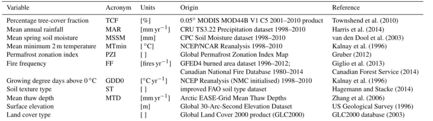
Table 1.Variables and datasets summary. Percentage tree-cover fraction indicates the proportion of land per grid cell covered by trees. Mean annual rainfall corresponds to the mean cumulative precipitation in millimetres over a year. Soil moisture is measured as water height equivalents in a 1.6 m soil column. Minimum temperature refers to air temperature at 2 m height. Permafrost zonation index shows the probability of a grid cell to have permafrost existing only in the most favourable conditions or nearly everywhere. Fire frequency is the averaged number of fire events per year. Growing degree days above 0◦C correspond to the sum of the mean daily temperatures at 2 m height above 0◦C through a year, using 6 h measurements. Soil texture describes the type of particles forming soil, ranging from sand to clay depending on the particle size. Mean thaw depth corresponds to millimetres of thawing soil during non-freezing days averaged per year. Surface elevation refers to the topographic altitude per grid cell in metres. Land cover type describes the type of vegetation and the density of the cover, independent of geo-climatic zone.
Variable Acronym Units Origin Reference
Percentage tree-cover fraction TCF [%] 0.05◦MODIS MOD44B V1 C5 2001–2010 product Townshend et al. (2010) Mean annual rainfall MAR [mm yr−1] CRU TS3.22 Precipitation dataset 1998–2010 Harris et al. (2014) Mean spring soil moisture MSSM [mm] CPC Soil Moisture dataset 1998–2010 van den Dool et al. (2003) Mean minimum 2 m temperature MTmin [◦C] NCEP/NCAR Reanalysis 1998–2010 Kalnay et al. (1996) Permafrost zonation index PZI [ ] Global Permafrost Zonation Index Map Gruber (2012) Fire frequency FF [fires yr−1] GFED4 burned area dataset 1996–2012; Giglio et al. (2013)
Canadian National Fire Database 1980–2014 Canadian Forest Service (2014) Growing degree days above 0◦C GDD0 [◦C yr−1] NCEP Reanalysis (NMC initialised) 1998–2010 Kalnay et al. (1996)
Soil texture type ST [ ] improved FAO soil type dataset Hagemann and Stacke (2014) Mean thaw depth MTD [mm yr−1] Arctic EASE-Grid Mean Thaw Depths Zhang et al. (2006) Surface elevation [m] Global 30-Arc-Second Elevation Dataset US Geological Survey (1996) Land cover type [ ] Global Land Cover 2000 product (GLC2000) GLC2000 database (2003)
To describe tree cover we make use of the percentage tree-cover fraction (%) from the MODIS MOD44B V1 C5 2001– 2010 product (Townshend et al., 2010). The MODIS tree-cover dataset has certain biases and limitations: it underesti-mates shrubs and small woody plants, as the product was cal-ibrated against trees above 5m tall (Bucini and Hanan, 2007); it never resolves 100 % of tree cover; it is not well resolved at low tree cover (Staver and Hansen, 2015); and may not be useful for differentiating over small ranges of tree cover (less than ca. 10 %; Hansen et al., 2003), as the use of classi-fication and regression trees (CARTs) to calibrate the dataset might introduce artificial discontinuities (Hanan et al., 2014). Regarding the particular case of the northern latitudes, an evaluation of the accuracy of the MODIS tree-cover fraction product pointed out that the dataset may not be suitable for detailed mapping and monitoring of tree cover at its finest resolution (500 m per pixel), especially for tree cover below 20 %, and that there might be a systematic bias over the Scan-dinavian region (Montesano et al., 2009). To overcome these limitations, we employ MODIS VCF data at a coarser resolu-tion (0.05◦, subsequently re-projected to 0.5◦), we aggregate for most of the analysis tree-cover values into three bins en-compassing the 0–20, 20–45, and 45–100 % ranges, and we exclude grid cells over Scandinavia from the analysis.
In our analysis, we investigate the use of an alternative dataset for temperatures, namely the CRU TS3.22 tmn prod-uct, for the years 1998–2010 (Harris et al., 2014). This dataset has a finer resolution and provides a more detailed picture of the ecosystem, albeit affected by a cold bias over Canada (see CRU TS 3.22 release notes, Harris et al., 2014). Nonetheless, it shows similar patterns to the NCEP/NCAR product. The two datasets are heavily linearly correlated,
al-though the CRU tmn product shows lower temperatures, es-pecially over eastern North Eurasia and eastern North Amer-ica. Since our analysis is independent of variable shifts, re-sults obtained using the CRU tmn product are essentially the same (see Supplement).
Within this setup, we assume that the dataset products are suitable for our investigation.
2.2 Data analysis
After filtering and dividing the dataset, we confirm the mul-timodality of the tree-cover distribution in high latitudes, as found by Scheffer et al. (2012) and in line with results from Xu et al. (2015), by optimising the fitting of different sums of Gaussian functions over the tree-cover fraction distribution (not shown). Next, we group all data grid cells according to the modal peaks into three states: “treeless”, where tree cover is smaller than 20 %, “open woodland”, with tree cover be-tween 20 and 45 %, and “forest”, where tree cover is greater than 45 %. The ensuing data analysis is aimed at two main purposes: to ascertain the impact of environmental variables on the tree cover, and to assess whether different vegetation states can be found under the same set of environmental vari-ables.
First, we evaluate the link between the eight environmen-tal factors on the tree-cover fraction distribution using GAMs (Miller et al., 2007). GAMs are data-driven statistical mod-els able to handle non-linear data structures (Hastie and Tib-shirani, 1986, 1990; Clark, 2013); their purpose is to ascer-tain the contributions and roles of the different variables, thus allowing a better understanding of the systems (Guisan et al., 2002). Each GAM test provides an estimate of the proportion of tree-cover fraction distribution that can be ex-plained through a smoothing of one or more environmen-tal variables (Staver et al., 2011b) – for instance, the for-mula TCF=s1(MTmin)+s2(MAR), with Gaussian family and identity link (see Supplement for further details on the implementation), is used to assess the contribution of mini-mum temperature and precipitation on the tree-cover fraction distribution. For each region, we repeatedly apply GAMs in-cluding different combinations of variables, and – to deter-mine whether the sample size influences the results – we use in turn either multiple random samples of 500 grid cells each, multiple random samples of 1000 grid cells each, or all the grid cells.
Subsequently, we analyse the conditional 2-dimensional phase space between the environmental variables to visualise whether intersections of vegetation states in each phase space are possible or not. To do so, we perform a kernel density estimation (KDE) of the joint distribution between the two environmental variables, conditioned to whether or not the corresponding data belong to the treeless, open woodland, or forest state, and we plot the KDE together with the envi-ronmental variable histograms. Kernel density estimates are used to approximate the probability density function under-lying a set of data (Silverman, 1981, 1986).
Next, after excluding growing degree days above 0◦C and mean thaw depth (see Sect. 3.2 for details), we look at the 6-dimensional (6-D) phase space formed by mean annual rainfall, mean spring soil moisture, mean minimum
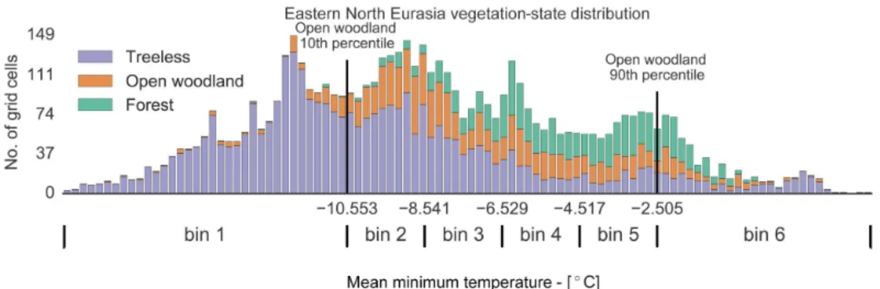
temper-ature, permafrost distribution, wildfire frequency, and soil texture, and we divide it into classes in the following man-ner. First, for every region, we divide the domain of each environmental variable into bins. To do so, we compute the 10th and 90th percentile of the three vegetation states with respect to every environmental variable except soil texture. Then, for the same variables, we select the second-lowest 10th and second-highest 90th percentiles; these two values are the boundaries of the first and last bin, while the range in between them is equally divided into bins: 5 for MTmin, MSSM, and MAR, and 3 for FF and PZI, as exemplified in Fig. 1 for MTmin; ST is instead divided according to the clay, sand, and loam groups. By doing so, we separate the range of an environmental variable where overlaps between the KDEs of the vegetation states are more likely to happen, from ranges where only one vegetation state is more likely to be found (respectively the central bins and the two most external ones). Second, we consider the partition of the 6-D phase space among the environmental variables generated by the so-computed bins. Each element of this partition is defined as a class, i.e. a class is a set of bins for the environ-mental variables. The idea behind this analysis is to split the 6-D environmental variable space into classes where environ-mental variables could be considered equal for all geograph-ical grid cells. The question, then, is whether the tree cover could be different under the same environmental conditions. Afterwards, to assess our research question, we associate every geographical grid cell of the boreal area with its veg-etation state and with the class corresponding to its environ-mental variable values. Subsequently, we select two types of areas of interest that correspond to possible alternative states:
– equivalent tree-cover states, defined as grid cells with
different vegetation states but the same environmental variable class, e.g. an open woodland grid cell and a forest grid cell, where all the environmental variables are in the same bins;
– fire-disturbed (FD) tree-cover states, defined as grid
cells with different vegetation state, where the environ-mental variables are in the same bins, except for wild-fire frequency, e.g. a forest grid cell with low wild-fire fre-quency and an open woodland grid cell with higher fire frequency but with the remaining environmental vari-ables in the same bins.
uni-Figure 1.Bin division of mean minimum temperature for eastern North Eurasia. The boundaries of the first and last bins are calculated using the second-lowest 10th percentile and second-highest 90th percentile of the three vegetation states, with respect to the environmental variable in use, having in mind that only one vegetation state is generally found below or above these thresholds, respectively. The remaining space is subdivided uniformly.
modality (Silverman, 1981; Hall and York, 2001). Finally, to ascertain that results cannot be explained by the internal vari-ability of the ecosystem alone, we compute the standard de-viation of the tree-cover fraction distribution for the period 2001–2010 over the same alternative-state grid cells, and we compare it with the distributions of the alternative states.
The entire analysis is carried out using Python 2.7.10, IPython 4.0.1, and RStudio 0.99.441.
3 Results
3.1 GAM results
Eastern North America is the region with the highest GAM results, with more than 80 % of the total deviance of tree cover explained, and every variable except fire frequency yielding higher results than in the other three regions. Ad-ditionally, the impact of environmental variables on the tree-cover fraction distribution depends on the region of interest, as can be seen in Table 2. For instance, soil texture influ-ence ranges from 9–15 to 42–52 % in western and eastern North America, respectively. A summary of GAM results us-ing random samples of 1000 grid cells is reported in Table 2. Growing degree days above 0◦C and mean minimum tem-perature are the environmental variables with the greatest in-fluence on the tree-cover distribution, with a combined effect ranging from 42 to 77 %, in line with literature, as tempera-ture is the main limiting factor for boreal forest (Bonan and Shugart, 1989). The next environmental variable in order of importance is permafrost distribution, with an impact rang-ing from 10–17 to 69–75 % dependrang-ing on the southern extent of continuous permafrost. Water availability, as expressed through the combined effect of rainfall and soil moisture, explains 26 to 62 % of the tree-cover distribution. The two variables have a similar influence when considered alone, although MAR always has a greater impact. The impact of wildfires depends heavily on the region of interest, with FF
Table 2.Summary of GAMs performed using random samples of 1000 grid cells each. The ranges represent the spread of results obtained with different samples, whereas the values in parenthe-sis correspond to the average from the samples. Statisticalpvalues are<0.0001 for every case. Percentages of explained deviance are a measure of the goodness of fit of each GAM (McCullagh and Nelder, 1989; Agresti, 1996). Reported values are related to the influence on tree-cover fraction distribution of mean annual rain-fall (MAR), mean minimum temperature (MTmin), growing de-gree days above 0◦C (GDD0), permafrost distribution (PZI), mean spring soil moisture (MSSM), wildfire occurrence frequency (FF), soil texture (ST), mean thawing depth (MTD). Values are divided within the four regions of interest, namely, eastern North Eurasia (EA_E), western North Eurasia (EA_W), eastern North America (NA_E), and western North America (NA_W).
Deviance of TCF Explained – %
Variables EA_E EA_W NA_E NA_W
MAR 24–30 (27) 28–38 (32) 51–57 (55) 28–36 (32) MSSM 12–20 (16) 20–29 (25) 43–53 (47) 11–21 (15) MTmin 36–44 (40) 23–31 (27) 70–75 (72) 36–43 (40) PZI 38–45 (42) 10–17 (13) 69–75 (71) 31–37 (34) FF 2–9 (5) 15–20 (18) 8–13 (11) 11–19 (14) GDD0 49–57 (54) 40–51 (46) 70–74 (71) 24–34 (28) ST 9–18 (12) 26–35 (30) 42–52 (47) 9–15 (12) MTD 21–33 (26) 27–37 (32) 39–46 (43) 18–30 (23) MAR+MSSM 26–31 (28) 29–41 (34) 56–62 (59) 31–38 (34) MTmin+GDD0 53–60 (56) 43–54 (49) 73–77 (75) 42–50 (46) PZI+FF 42–48 (46) 34–42 (36) 70–76 (73) 34–42 (38) All 60–67 (63) 52–58 (55) 80–85 (82) 59–65 (62)
contributing the lowest in eastern North Eurasia and the high-est in whigh-estern North Eurasia: 2–9 and 15–20 % respectively. Soil-related variables, namely soil texture and thaw depth, have a similar impact, generally around 30 %.
their combined effect is only slightly greater than the ef-fect of each factor alone. Overall, the combined efef-fect of all the environmental variables contributes to 52–67 % of the tree-cover fraction distribution, with the exception of eastern North America, where the cold temperatures, per-mafrost distribution, and rainfall gradients clearly dominate the tree-cover distribution and make up for almost 80 % of it (omitted from Table 2). We obtain similar results when com-bining temperature-related environmental variables (GDD0, MTmin) with water-related ones (MAR, MSSM).
Performing GAM analysis using all the grid cells or ran-dom samples of 1000 grid cells yields similar results, with explained deviances for the former case in between the ex-tremes of the latter, and always with statistical p value<
0.0001. On the other hand, using samples of 500 grid cells
can increase the explained portion of TCF distribution at the expense of statistical significance, due to higher p values,
and larger-scale applicability. Furthermore, the percentage of explained tree-cover fraction distribution is reduced (∼40 %
maximum combined deviance explained) if we perform the analysis on broader regions than the ones considered here, i.e. on the entire boreal area at once or on the individual con-tinents.
3.2 Phase-space analysis
Combining together environmental variables in phase space and performing a kernel density estimation of the joint distri-bution between the two environmental variables, conditioned to whether or not the corresponding data belong to the tree-less, open woodland, or forest state, it is possible to locate peaks in the distributions of the vegetation states.
In many phase-space regions, environmental conditions support only a single “dominant” vegetation state. For in-stance, low values of GDD0 clearly denote a peak in the distribution of the treeless state. Unfortunately, GDD0 does generally not separate well between the vegetation states in the central area of its distribution, and even when combined with other variables, a clear picture does not emerge. For this reason, and for its high correlation with MTmin (Pear-son’s correlation coefficient 0.78< r <0.94), GDD0 is not
used in the classification. Similarly, MTD is also excluded. Nonetheless, peaks of the KDEs are not always completely disjoint, and it is possible to find intersections between the KDEs of the different vegetation states, as for the case of mean annual rainfall and mean minimum temperature with values around 400 mm and−7◦C, respectively, where both
forest and open woodland are possible. This means that the same environmental conditions can lead to different vegeta-tion states, hinting at possible alternative states.
As a representative case, phase-space plots for eastern North Eurasia are shown in Fig. 2. Particularly, Fig. 2a rep-resents the KDE of the joint distribution between MAR and MTmin. Each colour is associated with a vegetation state: green for forest, orange for open woodland, and purple for
treeless. The isolines describe the probability of finding the three vegetation states under the specific environmental vari-ables regimes, with intense colours indicating higher proba-bilities. The marginal distributions are reported on the sides of the plot in the form of histograms. The intersections of iso-lines marked in Fig. 2a show phase-space regions where the same environmental conditions can lead to different vegeta-tion states. Similarly, Fig. 2b represents the KDE of the joint distribution between MSSM and GDD0, with highlighted ar-eas where a single dominant vegetation state is supported by the environmental variables.
Results vary by region, and a complete description of all the combinations between variables is beyond the scope of this paper. Suffice to say that extremes in the distributions of environmental variables are generally associated with a single vegetation state, as in Fig. 2b, whereas intermediate values allow for both single states and intersections (Fig. 2a and b, respectively). However, these intersections consider only two environmental variables at a time and they provide only part of the total picture. Results from the classification described and discussed in Sects. 2.2 and 3.3 cover all the environmental variables at once.
3.3 6-D phase-space classification
Figure 2.Representation of the KDEs of the three vegetation states in the phase space generated by mean minimum temperature and mean annual rainfall(a), and mean spring soil moisture and growing degree days above 0◦C(b), for eastern North Eurasia. Vegetation states are colour-coded as follows: green for forest, orange for open woodland, and purple for treeless. The isolines describe the probability of finding the three vegetation states under the specified environmental variables regimes, with intense colours indicating higher probabilities. Highlighted intersections in phase space represent areas with different vegetation states under the same environmental conditions(a), whereas the marked areas with only one dominant state hint at the unimodality of the underlying distribution (b). Marginal distributions for the variables are reported to the sides of the plots in the form of histograms.
Table 3.Summary of possible vegetation states, divided as monos-table, bismonos-table, and fire-disturbed. Fire-disturbed states have a higher fire regime than the indicated counterpart. Treeless always refers to TCF<20 %, open woodland to 20 %≤TCF<45 %, and forest to TCF≥45 %.
Monostable Bistable Fire-disturbed
Treeless Treeless – open Open woodland –
woodland FD treeless
Open woodland Forest – FD
open woodland
Forest Forest – open Open Woodland –
woodland FD forest
high. Precise values are reported in Table 4 (see Supplement). Soil texture is described as belonging to the sand, loam, or clay group. Permafrost is described as sparse, discontinuous, frequent, or continuous. Each environmental variable class contains two possible vegetation states, e.g. forest and open woodland, that are consistently found under the same speci-fied environmental regimes.
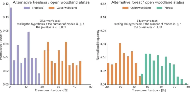
Table 4 and Fig. 3 pinpoint the conditions and locations, respectively, of the possible alternative tree-cover states in the boreal area. To test whether the distributions of the pos-sible alternative tree-cover states are multimodal, we employ the Silverman’s test. Each Silverman’s test assesses the hy-pothesis that the number of modes of the distributions of the alternative open woodland and treeless grid cells, and of the alternative open woodland and forest grid cells, is ≤1.
The tests show that the minimum number of modes to de-scribe the distributions is two, for both cases, withpvalues
smaller than 0.001 and 0.01, respectively. Figure 4 shows the
results of the Silverman’s tests on the distributions of the pos-sible alternative tree-cover states, confirming their bimodal-ity, together with the respective tree-cover distributions. It is clear in Fig. 4 that both cases exhibit a decrease in frequency around 20 and 45 % tree cover.
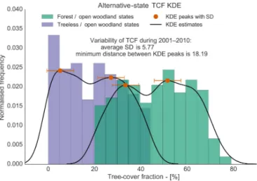
Furthermore, we test whether the tree-cover modes can be a product of internal variability alone. To do so, we fit the distributions of the possible alternative tree-cover states us-ing KDEs, we estimate the distances between the peaks of the distributions, and we compare them with the standard devi-ation of the tree-cover fraction distribution during the 2001– 2010 time interval, as a measure of variability. The minimum distance between peaks corresponding to different vegetation states is 18.19 percentage points (note that tree-cover fraction
is measured as a percentage), whereas the average standard deviation for the alternative-state grid cells is 5.77
percent-age points, with only one grid cell possessing a variability greater than 18 percentage points. Henceforth, the bimodal-ity of the alternative-state distributions cannot be explained by the variability of the tree-cover fraction alone. A compar-ison between the distributions of the alternative tree-cover states, the estimated modal peaks, and internal variability is presented in Fig. 5.
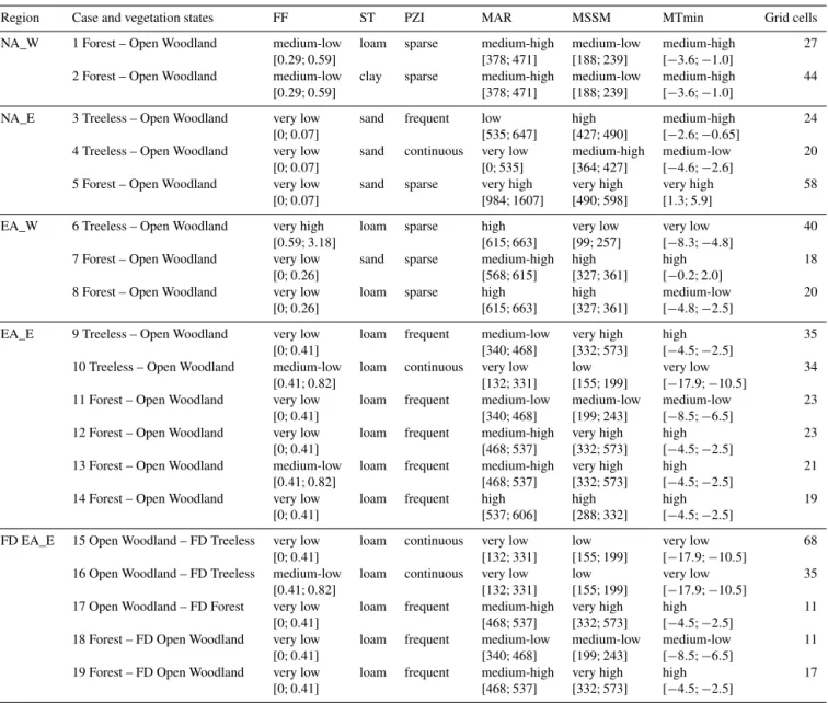
Table 4.Classes related to equivalent tree-cover states and fire-disturbed (FD) tree-cover states. The qualitative marks for fire frequency, mean annual rainfall, mean spring soil moisture, and mean minimum temperature are relative to the extremes of their distributions in the region of interest, and represent the bins into which the phase space is subdivided. Precise values for these bins are reported in brackets. Soil texture is described as belonging to the sand, loam, or clay group. Permafrost is described as sparse, discontinuous, frequent, or continuous. Each environmental variable class contains two possible vegetation states, e.g. forest and open woodland, that are consistently found under the same specified environmental regimes.
Region Case and vegetation states FF ST PZI MAR MSSM MTmin Grid cells
NA_W 1 Forest – Open Woodland medium-low loam sparse medium-high medium-low medium-high 27 [0.29;0.59] [378;471] [188;239] [−3.6; −1.0]
2 Forest – Open Woodland medium-low clay sparse medium-high medium-low medium-high 44 [0.29;0.59] [378;471] [188;239] [−3.6; −1.0]
NA_E 3 Treeless – Open Woodland very low sand frequent low high medium-high 24 [0;0.07] [535;647] [427;490] [−2.6; −0.65]
4 Treeless – Open Woodland very low sand continuous very low medium-high medium-low 20 [0;0.07] [0;535] [364;427] [−4.6; −2.6]
5 Forest – Open Woodland very low sand sparse very high very high very high 58 [0;0.07] [984;1607] [490;598] [1.3;5.9]
EA_W 6 Treeless – Open Woodland very high loam sparse high very low very low 40 [0.59;3.18] [615;663] [99;257] [−8.3; −4.8]
7 Forest – Open Woodland very low sand sparse medium-high high high 18 [0;0.26] [568;615] [327;361] [−0.2;2.0]
8 Forest – Open Woodland very low loam sparse high high medium-low 20 [0;0.26] [615;663] [327;361] [−4.8; −2.5]
EA_E 9 Treeless – Open Woodland very low loam frequent medium-low very high high 35 [0;0.41] [340;468] [332;573] [−4.5; −2.5]
10 Treeless – Open Woodland medium-low loam continuous very low low very low 34 [0.41;0.82] [132;331] [155;199] [−17.9; −10.5]
11 Forest – Open Woodland very low loam frequent medium-low medium-low medium-low 23 [0;0.41] [340;468] [199;243] [−8.5; −6.5]
12 Forest – Open Woodland very low loam frequent medium-high very high high 23 [0;0.41] [468;537] [332;573] [−4.5; −2.5]
13 Forest – Open Woodland medium-low loam frequent medium-high very high high 21 [0.41;0.82] [468;537] [332;573] [−4.5; −2.5]
14 Forest – Open Woodland very low loam frequent high high high 19
[0;0.41] [537;606] [288;332] [−4.5; −2.5]
FD EA_E 15 Open Woodland – FD Treeless very low loam continuous very low low very low 68 [0;0.41] [132;331] [155;199] [−17.9; −10.5]
16 Open Woodland – FD Treeless medium-low loam continuous very low low very low 35 [0.41;0.82] [132;331] [155;199] [−17.9; −10.5]
17 Open Woodland – FD Forest very low loam frequent medium-high very high high 11 [0;0.41] [468;537] [332;573] [−4.5; −2.5]
18 Forest – FD Open Woodland very low loam frequent medium-low medium-low medium-low 11 [0;0.41] [340;468] [199;243] [−8.5; −6.5]
19 Forest – FD Open Woodland very low loam frequent medium-high very high high 17 [0;0.41] [468;537] [332;573] [−4.5; −2.5]
medium or intermediate values for all the environmental vari-ables, whereas case number 6 shows high values for FF and MAR, but very low for MSSM and MTmin. The first cate-gory, with intermediate values, can be associated with tran-sition zones, when passing from an environmental variable class where only a single vegetation state is dominant, to a class where another state is dominant. As a result, the ob-served tree-cover fraction distribution can oscillate between the two states. The second category, on the other hand, re-lates to classes where at least one of the environmental vari-ables has a value contrasting with the remaining ones. For instance, in case 8, PZI, MAR, MSSM, and ST all possess
Figure 3.Possible alternative tree-cover states over North America (left) and North Eurasia (right). The bottom five panels represent a close-up of the areas of interest ordered from west to east. Legend to be interpreted as follows: for every entry in the legend, the first name refers to the observed vegetation state in a specific grid cell, the second name corresponds to the possible alternative state found elsewhere under the same environmental conditions. Fire-disturbed tree-cover states are only present eastern North Eurasia.
Figure 4.Tree-cover fraction distribution over the grid cells where equivalent or fire-disturbed open woodland and treeless states are found (left), and where equivalent or fire-disturbed open woodland and forest states are found (right). For each case the Silverman’s test verifies the hypothesis that the distribution is unimodal. Thepvalue is low in both cases, confirming the multimodality of the distributions.
category corresponds to the first one, but neither of the veg-etation states is found among equivalent tree-cover classes (case 15, although very similar to case 10).
Classification results suggest that environmental variables exert a strong, albeit sensitive, control over the tree-cover dis-tribution. Depending on the conditions, only one of the three
possible vegetation states is attained; for instance, in eastern North America, classes with very low mean annual rainfall and mean minimum temperature (MAR below 500 mm yr−1 and MTmin lower than−9◦C; see Supplement) are
Figure 5.The histogram shows the tree-cover fraction distributions of the possible alternative cover states compared with tree-cover fraction internal variability. Purple bars refer to treeless/open woodland states, and green to forest/open woodland states. The black lines and the orange dots represent the kernel density estimate fittings of these distributions and the locations of their modal peaks, respectively. Internal variability of the tree-cover fraction distribu-tion for the period 2001–2010, computed as the standard deviadistribu-tion of the distribution, is 5.77 percentage points, and is represented as the orange error-bars. The minimum distance between peaks cor-responding to different vegetation states is 18.19 percentage points and is higher than what internal variability could explain.
However, in transition zones with intermediate or contrast-ing conditions, it is possible to find multiple vegetation states with the same environmental regimes. In such zones, distur-bances could shift the system between the possible alterna-tive states. In this sense, fire is part of the environment both as a variable (Wirth, 2005; Schulze et al., 2005) and as a dis-turbance. Strong fire events in transition zones can determine which of two alternative states the system will fall into. On the other hand, changes due to fire events in a stable area should be reabsorbed with time, unless they are so dramatic as to produce changes in another main environmental vari-able, creating a new transition zone.
4 Discussion
The link between environmental variables and tree-cover fraction varies within the four boreal regions considered here, as described in Sect. 3.1, and is stronger in eastern North America, where the cold temperatures, permafrost distribu-tion, and rainfall gradients dominate the tree-cover distri-bution. Furthermore, the percentage of explained tree-cover fraction distribution is greatly reduced when performing the analysis on broader regions, such as the entire boreal area at once or on the single continents. We hypothesise that this is caused by the different species distribution across the re-gions and by the different species-specific adaptations to the
surrounding environment. For instance, North America is mainly dominated by “fire-embracing trees”, promoting the accumulation of fuel and the occurrence of high-intensity crown fires. On the other hand, Eurasia is populated by “fire-resistant trees” in its driest regions, i.e. eastern North Eurasia, where only surface fires are common, and “fire-avoider trees” in western North Eurasia, which burn less frequently due to the wetter climate of this region (Wirth, 2005; Rogers et al., 2015). As a result, despite the environmental variables hav-ing different distributions, the general response of the tree-cover distribution in the four regions is similar, but the im-pact of each individual environmental variable varies within the regions.
Minimum temperatures and growing degree days are the most influential environmental variables for the boreal tree-cover fraction distribution, as can be seen in Table 2. Nonetheless, their combined effect does not fully explain the tree-cover distribution, as a more diverse set of variables and feedbacks plays a role. Additionally, the environmental vari-ables are not independent of each other, and hence the com-bined impact of multiple variables does not correspond to the sum of the single terms. Furthermore, the overall effect of the environmental variables is not able to fully explain the tree-cover distribution. We hypothesise this can be linked mainly to three possible causes. First, missing factors in the evaluation, for instance insect outbreaks, which are linked to climate and play an important role in the boreal forest dy-namic (Bonan and Shugart, 1989), or grazing from animals (Wal, 2006; Olofsson et al., 2010). Second, deficiencies in the datasets used, such as the underestimation of fire events in the boreal region (Mangeon et al., 2015), and the limited timespan of satellite observations, as fire return intervals in high latitudes can exceed 200 years (Wirth, 2005). Third, supported by the multimodality of the boreal forest (Scheffer et al., 2012; Xu et al., 2015) and by the results presented in Sect. 3.3, the presence of areas where the system is in dif-ferent alternative stable states under the same environmental conditions.
shift the vegetation from one state to the other, as in the case of fire-disturbed tree-cover states. Particularly, eastern North Eurasia is the region with the greatest extent of possible alter-native tree-cover states, and it is the only region where fire-disturbed states are found, hinting at a greater susceptibility of its forest resilience.
Environmental conditions control the tree-cover distribu-tion in high latitudes, pushing its vegetadistribu-tion towards three distinct tree-cover states. This hints at the presence of feed-backs between the vegetation and the environment, which are able to stabilise the vegetation cover in three differ-ent ways. However, the environmdiffer-ent is influenced by the forest cover state through albedo, water evapotranspiration (Brovkin et al., 2009), and nutrient recycling. Thus, changes in climate and environmental variables will trigger feedbacks from the vegetation that can either further amplify or dampen the initial changes. In particular, areas of reduced resilience where alternative tree-cover states are found, i.e. what we call transition zones, will be affected. As the classification results suggest, environmental variables drive the ecosystem towards seemingly stable states and away from intermedi-ate unstable ones, resulting in the multimodality of the tree cover. Thus, disturbances in transition zones could cause a rapid ecosystem shift regarding tree cover. Henceforth, it is important to better understand the interplay between environ-mental variables and tree cover.
Additionally, there are other factors playing a role in the dynamics of the boreal forest, both at local and larger scales. For instance, the understory vegetation acts as an impor-tant driver of soil fertility, influencing plant growth and tree seedling establishment (Bonan and Shugart, 1989; Nilsson and Wardle, 2005). An increased nitrogen deposition may promote accumulation of organic matter and carbon in bo-real forest (Mäkipää, 1995). At the same time, its effects on the forest floor and soil processes might decrease for-est growth (Mäkipää, 1995). Despite its importance, there is a lack of knowledge regarding the impact of understory interactions at large spatial scales, and the contribution of climate-change drivers (Nilsson and Wardle, 2005). For these reasons we could not take it into account in our study. An-other missing factor is nitrogen (N), as plant growth in the boreal forest is thought to be generally N-limited (Mäkipää, 1995). Additionally, herbivore grazing is also influenced by N fertilisation (Ball et al., 2000), with the potential to affect feedbacks involving soil nutrient cycle and plant regenera-tion (Wal, 2006). However, globally distributed datasets for N availability and grazing pressure suitable for our analy-sis are not yet available. Local topography also plays a role, as the low solar elevation angle at high latitudes accentu-ates the effect of ground characteristics such as slope and aspect (Rydén and Kostov, 1980; Bonan and Shugart, 1989; Rieger, 2013), affecting temperature and soil moisture. Fi-nally, micro-topography, such as shelter from boulders, can increase resistance to disturbances by creating small-scale
refugia (Schmalholz and Hylander, 2011), thus locally in-creasing the resilience of the forest.
In the context of climate change, understanding transition zones at large scales is necessary for assessing future projec-tions of vegetation cover. Climate change is impacting the boreal area more rapidly and intensely than other regions on Earth; for instance, surface temperature has been increas-ing approximately twice as fast as the global average (IPCC, 2013). Temperature is a key variable in this region, as it is connected with tree growth and mortality cycles, with per-mafrost thawing and the hydrological cycle, and with distur-bances, such as wildfires and insect outbreaks (Judy et al., 2005; Wolken et al., 2011; Johnstone et al., 2010; Schef-fer et al., 2012; D’Orangeville et al., 2016). Particularly, air and surface warming can increase the frequency and extent of severe fires (Flannigan et al., 2005; Balshi et al., 2009; Johnstone et al., 2010), and promote more favourable condi-tions for insect outbreaks (Volney and Fleming, 2000). At the same time, climate-change influences the resilience of boreal forest stands (Johnstone et al., 2010), making them more susceptible to abrupt shifts due to disturbances. As tem-perature increases and permafrost thaws, it is more likely to find intermediate conditions where alternative tree-cover states are possible. For instance, a study on the southern part of the eastern North American boreal forest has shown that an increased disturbance regime, together with the su-perimposition of fires and defoliating insect outbreaks, can cause a shift between alternative vegetation states (Jasinski and Payette, 2005). Furthermore, there is strong evidence that certain types of extreme events, mostly heatwaves and precipitation extremes, are increasing under the effect of cli-mate change (Orlowsky and Seneviratne, 2012; Coumou and Rahmstorf, 2012). Such events could foster areas with con-trasting environmental conditions, further weakening the sta-bility of the boreal ecosystem, and increasing its susceptibil-ity to shifts.
5 Conclusions
Through the analysis of generalised additive models, we find that the environment exerts a strong control over the tree-cover distribution, forcing it into distinct tree-tree-cover states. Nonetheless, the tree-cover state is not always uniquely de-termined by the variables at use. Furthermore, the response of vegetation to the environment varies in the four regions considered: eastern North America, western North America, eastern North Eurasia, and western North Eurasia.
low temperature, or with intermediate environmental values. In regions under these environmental conditions, the tree cover exhibits a reduced resilience, as it can shift between alternative states if subject to forcing.
As fires can shift the tree cover from one vegetation state to another in regions of reduced resilience, we find support for the hypothesis that a strong fire disturbance could perma-nently change the state of the ecosystem, by the combined effect of a shift in tree cover and its potential feedbacks on the environment.
Finally, we find that regions with possible alternative tree-cover states encompass only a small percentage of the boreal area (∼5 %). However, since temperature and
temperature-related environmental variables exert the strongest control on the tree-cover distribution and its modes, temperature changes could greatly affect forest resilience and cause an expansion of regions with alternative tree-cover states.
In the context of climate change, a gradual expansion of transition zones with reduced resilience could lead to re-gional ecosystem shifts with a significant impact not only on the structure and functioning of the boreal forest, but also on its climate.
6 Data availability
All data, scripts, and information necessary to reproduce the authors’ work are archived by the Max Planck Institute for Meteorology. They are accessible at http://hdl.handle.net/ 11858/00-001M-0000-002C-4F6F-3 or by contacting Car-ola Kauhs at [email protected].
Information about the Supplement
All data necessary to reproduce the paper are provided in the Supplement.
The Supplement related to this article is available online at doi:10.5194/bg-14-511-2017-supplement.
Author contributions. Both authors designed the research. Beni-amino Abis performed the research. Both authors contributed to the discussion and interpretation of the results. Beniamino Abis wrote the first draft of the manuscript and both authors contributed to its final draft.
Competing interests. The authors declare that they have no conflict of interest.
Acknowledgements. We would like to thank the Integrated Cli-mate Data Center (ICDC, http://icdc.cen.uni-hamburg.de/) of the University of Hamburg for helping with the retrieval of datasets. We thankfully acknowledge Gitta Lasslop for helping us review the manuscript, and Fabio Cresto Aleina for his useful comments. We also thank the International Max Planck Research School on Earth System Modelling (IMPRS-ESM) for supporting this work. Finally, we thank our editor A. Ito and three anonymous referees for their constructive comments on the paper.
The article processing charges for this open-access publication were covered by the Max Planck Society.
Edited by: A. Ito
Reviewed by: three anonymous referees
References
Agresti, A.: Categorical data analysis, 996, New York, John Wiley & Sons, 1996.
Juday, G. P., Barber, V., Duffy, P., Linderholm, H., Rupp, S., Spar-row, S., Vaganov, E., Yarie, J., Berg, E., D’Arrigo, R., Eggerts-son, O., Furyaev, V. V., Hogg, E. H., Huttunen, S., Jacoby, G.,d Kaplunov, V. Y., Kellomaki, S., Kirdyanov, A. V., Lewis, C. E., Linder, S., Naurzbaev, M. M., Pleshikov, F. I., Runesson, U. T., Savva, Y. V., Sidorova, O. V., Stakanov, V. D., Tchebakova, N. M., Valendik, E. F., Vedrova, E. F., and Wilmking, M: Forests, land management and agriculture, Arctic Climate Impact Assess-ment, 781–862, 2005.
Ball, J. P., Danell, K., and Sunesson, P.: Response of a herbivore community to increased food quality and quantity: an experiment with nitrogen fertilizer in a boreal forest, J. Appl. Ecol., 37, 247– 255, 2000.
Balshi, M. S., Mcguire, A. D., Duffy, P., Flannigan, M., Walsh, J., and Melillo, J.: Assessing the response of area burned to chang-ing climate in western boreal North America uschang-ing a Multivariate Adaptive Regression Splines (MARS) approach, Glob. Change Biol., 15, 578–600, 2009.
Barona, E., Ramankutty, N., Hyman, G., and Coomes, O. T.: The role of pasture and soybean in deforestation of the Brazil-ian Amazon, Environ. Res. Lett., 5, 024002, doi:10.1088/1748-9326/5/2/024002, 2010.
Baudena, M., Dekker, S. C., van Bodegom, P. M., Cuesta, B., Hig-gins, S. I., Lehsten, V., Reick, C. H., Rietkerk, M., Scheiter, S., Yin, Z., Zavala, M. A., and Brovkin, V.: Forests, savannas, and grasslands: bridging the knowledge gap between ecology and Dynamic Global Vegetation Models, Biogeosciences, 12, 1833– 1848, doi:10.5194/bg-12-1833-2015, 2015.
Bel, G., Hagberg, A., and Meron, E.: Gradual regime shifts in spatially extended ecosystems, Theor. Ecol., 5, 591–604, doi:10.1007/s12080-011-0149-6, 2012.
Benninghoff, W. S.: Interaction of vegetation and soil frost phenom-ena, Arctic, 5, 34–44, 1952.
Bonan, G. B.: Environmental factors and ecological processes con-trolling vegetation patterns in boreal forests, Landscape Ecol., 3, 111–130, doi:10.1007/BF00131174, 1989.
Bonan, G. B. and Shugart, H. H.: Environmental Factors and Eco-logical Processes in Boreal Forests, Annu. Rev. Ecol. Syst., 20, 1–28, doi:10.1146/annurev.es.20.110189.000245, 1989. Bonan, G. B., Pollard, D., and Thompson, S. L.: Effects of
bo-real forest vegetation on global climate, Nature, 359, 716–718, doi:10.1038/359716a0, 1992.
Bond, W. J. and Midgley, G. F.: Carbon dioxide and the uneasy interactions of trees and savannah grasses, Philos. T. Roy. Soc. B, 367, 601–612, 2012.
Brando, P. M., Balch, J. K., Nepstad, D. C., Morton, D. C., Putz, F. E., Coe, M. T., Silvério, D., Macedo, M. N., Davidson, E. A., Nóbrega, C. C., Alencara, A., and Soares-Filho, B. S.: Abrupt increases in Amazonian tree mortality due to drought–fire inter-actions, P. Natl. Acad. Sci. USA, 111, 6347–6352, 2014. Brouwers, N. C., Mercer, J., Lyons, T., Poot, P., Veneklaas, E., and
Hardy, G.: Climate and landscape drivers of tree decline in a Mediterranean ecoregion, Ecol. Evol., 3, 67–79, 2013.
Brovkin, V., Raddatz, T., Reick, C. H., Claussen, M., and Gayler, V.: Global biogeophysical interactions between forest and climate, Geophys. Res. Lett., 36, doi:10.1029/2009GL037543, 2009. Bryan, J. E., Shearman, P. L., Asner, G. P., Knapp, D. E., Aoro, G.,
and Lokes, B.: Extreme differences in forest degradation in Bor-neo: comparing practices in Sarawak, Sabah, and Brunei, PloS one, 8, e69679, doi:10.1371/journal.pone.0069679, 2013. Bucini, G. and Hanan, N. P.: A continental-scale analysis of tree
cover in African savannas, Global Ecol. Biogeogr., 16, 593–605, 2007.
Canadian Forest Service: Canadian National Fire Database – Agency Fire Data, Natural Resources Canada, Canadian Forest Service, Northern Forestry Centre, Edmonton, Alberta, available at: http://cwfis.cfs.nrcan.gc.ca/ha/nfdb (last access: 24 January 2017), 2014.
Clark, M.: Generalized additive models: getting started with addi-tive models in R, Center for Social Research, University of Notre Dame, 2013.
Coumou, D. and Rahmstorf, S.: A decade of weather extremes, Na-ture Climate Change, 2, 491–496, 2012.
Crowther, T. W., Glick, H. B., Covey, K. R., Bettigole, C., May-nard, D. S., Thomas, S. M., Smith, J. R., Hintler, G., Duguid, M. C., Amatulli, G., Tuanmu, M.-N., Jetz, W., Salas, C., Stam, C., Piotto, D., Tavani, R., Green, S., Bruce, G., Williams, S. J., Wiser, S. K., Huber, M. O., Hengeveld, G. M., Nabuurs, G.-J., Tikhonova, E., Borchardt, P., Li, C.-F., Powrie, L. W., Fischer, M., Hemp, A., Homeier, J., Cho, P., Vibrans, A. C., Umunay, P. M., Piao, S. L., Rowe, C. W., Ashton, M. S., Crane, P. R., and Bradford, M. A.: Mapping tree density at a global scale, Nature, 525, 201–205, 2015.
DeFries, R. S., Rudel, T., Uriarte, M., and Hansen, M.: Deforesta-tion driven by urban populaDeforesta-tion growth and agricultural trade in the twenty-first century, Nat. Geosci., 3, 178–181, 2010. de L. Dantas, V., Batalha, M. A., and Pausas, J. G.: Fire drives
func-tional thresholds on the savanna-forest transition, Ecology, 94, 2454–2463, 2013.
D’Orangeville, L., Duchesne, L., Houle, D., Kneeshaw, D., Côté, B., and Pederson, N.: Northeastern North America as a potential refugium for boreal forests in a warming climate, Science, 352, 1452–1455, doi:10.1126/science.aaf4951, 2016.
Eugster, W., Rouse, W. R., Pielke Sr, R. A., Mcfadden, J. P., Baldoc-chi, D. D., Kittel, T. G. F., Chapin, F., Stuart Liston, G. E., Vidale,
P. L., Vaganov, E., and Chambers, S.: Land–atmosphere energy exchange in Arctic tundra and boreal forest: available data and feedbacks to climate, Glob. Change Biol., 6, 84–115, 2000. Favier, C., Aleman, J., Bremond, L., Dubois, M. A., Freycon, V.,
and Yangakola, J.-M.: Abrupt shifts in African savanna tree cover along a climatic gradient, Global Ecol. Biogeogr., 21, 787–797, 2012.
Flannigan, M.: Fire evolution split by continent, Nat. Geosci., 8, 167–168, 2015.
Flannigan, M. D., Logan, K. A., Amiro, B. D., Skinner, W. R., and Stocks, B.: Future area burned in Canada, Climatic Change, 72, 1–16, 2005.
Fletcher, M.-S., Wood, S. W., and Haberle, S. G.: A fire-driven shift from forest to non-forest: evidence for alternative stable states?, Ecology, 95, 2504–2513, 2014.
Gauthier, S., Bernier, P., Kuuluvainen, T., Shvidenko, A., and Schepaschenko, D.: Boreal forest health and global change, Sci-ence, 349, 819–822, 2015.
Giglio, L., Randerson, J. T., and van der Werf, G. R.: Analy-sis of daily, monthly, and annual burned area using the fourth-generation global fire emissions database (GFED4), J. Geophys. Res.-Biogeo., 118, 317–328, doi:10.1002/jgrg.20042, 2013. GLC2000 database: The Global Land Cover Map for the Year 2000,
European Commission Joint Research Centre, available at: http: //forobs.jrc.ec.europa.eu/products/glc2000/products.php (last ac-cess: 24 January 2017), 2003.
Good, P., Harper, A., Meesters, A., Robertson, E., and Betts, R.: Are strong fire–vegetation feedbacks needed to explain the spa-tial distribution of tropical tree cover?, Global Ecol. Biogeogr., 25, 16–25, 2016.
Gruber, S.: Derivation and analysis of a high-resolution estimate of global permafrost zonation, The Cryosphere, 6, 221–233, doi:10.5194/tc-6-221-2012, 2012.
Guisan, A., Edwards, T. C., and Hastie, T.: Generalized linear and generalized additive models in studies of species distributions: setting the scene, Ecol. Modell., 157, 89–100, 2002.
Hagemann, S. and Stacke, T.: Impact of the soil hydrology scheme on simulated soil moisture memory, Clim. Dynam., 44, 1731– 1750, 2014.
Hall, P. and York, M.: On the calibration of Silverman’s test for multimodality, Stat. Sinica, 11, 515–536, 2001.
Hanan, N. P., Tredennick, A. T., Prihodko, L., Bucini, G., and Dohn, J.: Analysis of stable states in global savannas: Is the CART pulling the horse?, Global Ecol. Biogeogr., 23, 259–263, doi:10.1111/geb.12122, 2014.
Hansen, M. C., DeFries, R. S., Townshend, J. R., Carroll, M., DiM-iceli, C., and Sohlberg, R. A.: Global percent tree cover at a spa-tial resolution of 500 meters: First results of the MODIS vegeta-tion continuous fields algorithm, Earth Interact., 7, 1–15, 2003. Harris, I., Jones, P. D., Osborn, T. J., and Lister, D. H.: CRU TS3.22:
Climatic Research Unit (CRU) Time-Series (TS) Version 3.22 of High Resolution Gridded Data of Month-by-month Variation in Climate (January 1901–December 2013), University of East Anglia Climatic Research Unit, NCAS British Atmospheric Data Centre, 24 September 2014, doi:10.1002/joc.3711, 2014. Hastie, T. J. and Tibshirani, R. J.: Generalized Additive Models
(with discussion), Stat. Sci., 1, 297–318, 1986.
Havranek, W. M. and Tranquillini, W.: Physiological processes dur-ing winter dormancy and their ecological significance, Ecophys-iology of coniferous forests, 95–124, 1995.
Heinselman, M. L.: Fire intensity and frequency as factors in the distribution and structure of northern ecosystems [Canadian and Alaskan boreal forests, Rocky Mountain subalpine forests, Great Lakes-Acadian forests, includes history, management, Canada, USA], USDA Forest Service General Technical Report WO, 1981.
Hengeveld, G. M., Nabuurs, G.-J., Didion, M., van den Wyngaert, I., Clerkx, A. P. P. M. S., and Schelhaas, M.-J.: A Forest Manage-ment Map of European Forests, Ecol. Soc., 17, doi:10.5751/ES-05149-170453, 2012.
Higgins, S. I., Bond, W. J., February, E. C., Bronn, A., Euston-Brown, D. I. W., Enslin, B., Govender, N., Rademan, L., O’Regan, S., Potgieter, A. L. F., Scheiter, S., Sowry, R., Trol-lope, L., and TrolTrol-lope, W. S. W.: Effects of four decades of fire manipulation on woody vegetation structure in savanna, Ecology, 88, 1119–1125, 2007.
Hirota, M., Hlmgren, M., Van Nes, E. H., and Scheffer, M.: Global Resilience of Tropical Forest and Savanna to Critical Transitions, Science, 334, 232–235, doi:10.1126/science.1210657, 2011. Huntley, B.: The responses of vegetation to past and future
cli-mate changes, in: Global change and Arctic terrestrial ecosys-tems, 290–311, Springer, 1997.
Huntley, B., Cramer, W., Morgan, A. V., Prentice, H. C., and Allen, J. R.: Past and future rapid environmental changes: the spatial and evolutionary responses of terrestrial biota, 47, Springer Sci-ence & Business Media, 2013.
Hyvönen, R., Ågren, G. I., Linder, S., Persson, T., Cotrufo, M. F., Ekblad, A., Freeman, M., Grelle, A., Janssens, I. A., Jarvis, P. G., Kellomäki, S., Lindroth, A., Loustau, D., Lundmark, T., Norby, R. J., Oren, R., Pilegaard, K., Ryan, M. G., Sigurdsson, B. D., Strömgren, M., van Oijen, M., and Wallin, G.: The likely im-pact of elevated [CO2], nitrogen deposition, increased tempera-ture and management on carbon sequestration in temperate and boreal forest ecosystems: a literature review, New Phytol., 173, 463–480, 2007.
IPCC: Climate Change 2013: The Physical Science Basis. Contri-bution of Working Group I to the Fifth Assessment Report of the Intergovernmental Panel on Climate Change, Cambridge Uni-versity Press, Cambridge, United Kingdom and New York, NY, USA, doi:10.1017/CBO9781107415324, 2013.
Jasinski, J. P. and Payette, S.: The creation of alternative sta-ble states in the southern boreal forest, Quebec, Canada, Ecol. Monogr., 75, 561–583, 2005.
Johnstone, J. F., Chapin, F. S., Hollingsworth, T. N., Mack, M. C., Romanovsky, V., and Turetsky, M.: Fire, climate change, and for-est resilience in interior Alaska, Can. J. Forfor-est Res., 40, 1302– 1312, 2010.
Kalnay, E., Kanamitsu, M., Kistler, R., Collins, W., Deaven, D., Gandin, L., Iredell, M., Saha, S., White, G., Woollen, J., Zhu, Y., Leetmaa, A., Reynolds, B., Chelliah, M., Ebisuzaki, W., Higgins, W., Janowiak, J., Mo, K. C., Ropelewski, C., Wang, J., Jenne, R., and Joseph, D.: The NCEP/NCAR 40-year reanalysis project, NCEP Reanalysis data provided by the NOAA/OAR/ESRL PSD, Boulder, Colorado, USA, available at: http://www.esrl.noaa.gov/ psd/ (last access: 24 January 2017), 1996.
Kenkel, N. C., Walker, D. J., Watson, P. R., Caners, R. T., and Las-tra, R. A.: Vegetation Dynamics in Boreal Forest Ecosystems, Coenoses, 12, 97–108, 1997.
Kenneth Hare, F. and Ritchie, J. C.: The boreal bioclimates, Geogr. Rev., 333–365, 1972.
Lasslop, G., Brovkin, V., Reick, C., Bathiany, S., and Kloster, S.: Multiple stable states of tree cover in a global land surface model due to a fire-vegetation feedback, Geophys. Res. Lett., 43, 6324– 6331, 2016.
Lindner, M., Maroschek, M., Netherer, S., Kremer, A., Barbati, A., Garcia-Gonzalo, J., Seidl, R., Delzon, S., Corona, P., Kolström, M., Lexer, M. J., and Marchetti, M,: Climate change impacts, adaptive capacity, and vulnerability of European forest ecosys-tems, Forest Ecol. Manag., 259, 698–709, 2010.
Lloyd, J. and Veenendaal, E. M.: Are fire mediated feedbacks burn-ing out of control?, Biogeosciences Discuss., doi:10.5194/bg-2015-660, in review, 2016.
Mäkipää, R.: Effect of nitrogen input on carbon accumulation of boreal forest soils and ground vegetation, Forest Ecol. Manag., 79, 217–226, 1995.
Malhi, Y., Roberts, J. T., Betts, R. A., Killeen, T. J., Li, W., and Nobre, C. A.: Climate change, deforestation, and the fate of the Amazon, Science, 319, 169–172, 2008.
Mangeon, S., Field, R., Fromm, M., McHugh, C., and Voulgarakis, A.: Satellite versus ground-based estimates of burned area: A comparison between MODIS based burned area and fire agency reports over North America in 2007, The Anthropocene Review, 3, 76–92, doi:10.1177/2053019615588790, 2015.
May, R. M.: Thresholds and breakpoints in ecosystems with a mul-tiplicity of stable states, Nature, 269, 471–477, 1977.
McCullagh, P. and Nelder, J. A.: Generalized linear models, CRC press, 37, 1989.
Michaelian, M., Hogg, E. H., Hall, R. J., and Arsenault, E.: Mas-sive mortality of aspen following severe drought along the south-ern edge of the Canadian boreal forest, Glob. Change Biol., 17, 2084–2094, 2011.
Miller, J., Franklin, J., and Aspinall, R.: Incorporating spatial de-pendence in predictive vegetation models, Ecol. Modell., 202, 225–242, 2007.
Mills, A. J., Milewski, A. V., Fey, M. V., Gröngröft, A., Petersen, A., and Sirami, C.: Constraint on woody cover in relation to nutrient content of soils in western southern Africa, Oikos, 122, 136–148, 2013.
Montesano, P. M., Nelson, R. F., Sun, G., Margolis, H. A., Kerber, A., and Ranson, K. J.: MODIS tree cover validation for the cir-cumpolar taiga–tundra transition zone, Remote Sens. Environ., 113, 2130–2141, 2009.
Moreira, A. G.: Effects of fire protection on savanna structure in Central Brazil, J. Biogeogr., 27, 1021–1029, 2000.
Nilsson, M.-C. and Wardle, D. A.: Understory vegetation as a for-est ecosystem driver: evidence from the northern Swedish boreal forest, Front. Ecol. Environ., 3, 421–428, 2005.
Olofsson, J., Moen, J., and Östlund, L.: Effects of reindeer on bo-real forest floor vegetation: Does grazing cause vegetation state transitions?, Basic Appl. Ecol., 11, 550–557, 2010.