GMDD
3, 2439–2476, 2010The Fire INventory from NCAR (FINN)
C. Wiedinmyer et al.
Title Page
Abstract Introduction
Conclusions References
Tables Figures
◭ ◮
◭ ◮
Back Close
Full Screen / Esc
Printer-friendly Version Interactive Discussion
Discussion
P
a
per
|
Dis
cussion
P
a
per
|
Discussion
P
a
per
|
Discussio
n
P
a
per
|
Geosci. Model Dev. Discuss., 3, 2439–2476, 2010 www.geosci-model-dev-discuss.net/3/2439/2010/ doi:10.5194/gmdd-3-2439-2010
© Author(s) 2010. CC Attribution 3.0 License.
Geoscientific Model Development Discussions
This discussion paper is/has been under review for the journal Geoscientific Model Development (GMD). Please refer to the corresponding final paper in GMD if available.
The Fire INventory from NCAR (FINN) – a
high resolution global model to estimate
the emissions from open burning
C. Wiedinmyer1, S. K. Akagi2, R. J. Yokelson2, L. K. Emmons1, J. A. Al-Saadi3, J. J. Orlando1, and A. J. Soja4
1
National Center for Atmospheric Research, Boulder, CO, USA
2
University of Montana, Department of Chemistry, Missoula, MT, USA
3
NASA Headquarters, Washington DC, USA
4
National Institute of Aerospace, NASA Langley Research Center, Hampton, VA, USA
Received: 3 December 2010 – Accepted: 9 December 2010 – Published: 23 December 2010
Correspondence to: C. Wiedinmyer ([email protected])
GMDD
3, 2439–2476, 2010The Fire INventory from NCAR (FINN)
C. Wiedinmyer et al.
Title Page
Abstract Introduction
Conclusions References
Tables Figures
◭ ◮
◭ ◮
Back Close
Full Screen / Esc
Printer-friendly Version Interactive Discussion
Discussion
P
a
per
|
Dis
cussion
P
a
per
|
Discussion
P
a
per
|
Discussio
n
P
a
per
|
Abstract
The Fire INventory from NCAR version 1.0 (FINNv1) provides daily, 1 km resolution, global estimates of the trace gas and particle emissions from open burning of biomass, which includes wildfire, agricultural fires, and prescribed burning and does not include biofuel use and trash burning. Emission factors used in the calculations have been
up-5
dated with recent data, particularly for the non-methane organic compounds (NMOC). The resulting global annual NMOC emission estimates are as much as a factor of 5 greater than some prior estimates. Chemical speciation profiles, necessary to allocate the total NMOC emission estimates to lumped species for use by chemical transport models, are provided for three widely used chemical mechanisms: SAPRC99,
GEOS-10
CHEM, and MOZART-4. Using these profiles, FINNv1 also provides global estimates of key organic compounds, including formaldehyde and methanol. The uncertainty in the FINNv1 emission estimates are about a factor of two; but, the estimates agree closely with other global inventories of biomass burning emissions for CO, CO2, and other species with less variable emission factors. FINNv1 emission estimates have
15
been developed specifically for modeling atmospheric chemistry and air quality in a consistent framework at scales from local to global. The product is unique because of the high temporal and spatial resolution, global coverage, and the number of species estimated. FINNv1 can be used for both hindcast and forecast or near-real time model applications and the results are being critically evaluated with models and observations
20
whenever possible.
1 Introduction
Open biomass burning, which for this study includes wildfires, agricultural burning, and managed burns and not biofuel use or trash burning, makes up an important part of the total global emissions of both trace gases and particulate matter. According to the
25
GMDD
3, 2439–2476, 2010The Fire INventory from NCAR (FINN)
C. Wiedinmyer et al.
Title Page
Abstract Introduction
Conclusions References
Tables Figures
◭ ◮
◭ ◮
Back Close
Full Screen / Esc
Printer-friendly Version Interactive Discussion
Discussion
P
a
per
|
Dis
cussion
P
a
per
|
Discussion
P
a
per
|
Discussio
n
P
a
per
|
biomass burning produced 51% of the global carbon monoxide (CO) emissions for 2000 and 20% of the oxides of nitrogen (NOx) emissions. Current emission inventories
estimate that open biomass burning (not including waste burning) emits 26–73% of global emissions of primary fine organic particulate matter (PM) and 33–41% of global fine black carbon (BC) PM emissions (Bond et al., 2004; Andreae and Rosenfeld,
5
2008).
Although episodic in nature and highly variable, open biomass burning emissions can contribute to local, regional, and global air quality problems and climate forcings (Crutzen and Andreae, 1990). The emissions of PM can degrade visibility (e.g., McK-eeking et al., 2006) and cause health problems (e.g., Pope and Dockery, 2006).
Gas-10
phase components in fire plumes, including non-methane organic compounds (NMOC) and NOx, can react downwind of the fire location and contribute to the chemistry that
forms ozone (e.g., Pfister et al., 2008). Carbon dioxide released to the atmosphere from largescale burning may have important implications for the carbon cycle (e.g., IPCC 2007; Wiedinmyer and Neff, 2007). Due to the importance of these emissions,
15
reasonable estimates of open burning emissions are critical to characterizing air quality problems, understanding in situ measurements, and simulating chemistry and climate. There have been many efforts to estimate the emissions of trace gases and par-ticles from fires. Emissions from individual fire events have been calculated using site-specific information (e.g., the 2002 Biscuit Fire in Oregon, Campbell et al., 2007;
20
the 2003 fires in Southern California, Muhle et al., 2007). Regional emission estimates have been created for specific time periods: for example, Michel et al. (2005) produced a fire emissions inventory for Asia for March–May 2001 in support of a major field campaign. Other inventories predict regional emissions over longer time periods (e.g., Lavoue et al., 2000; Soja et al., 2004; Wiedinmyer et al., 2006; Larkin et al., 2009).
25
GMDD
3, 2439–2476, 2010The Fire INventory from NCAR (FINN)
C. Wiedinmyer et al.
Title Page
Abstract Introduction
Conclusions References
Tables Figures
◭ ◮
◭ ◮
Back Close
Full Screen / Esc
Printer-friendly Version Interactive Discussion
Discussion
P
a
per
|
Dis
cussion
P
a
per
|
Discussion
P
a
per
|
Discussio
n
P
a
per
|
species representative of the late 1990s. Duncan et al. (2003) estimated global CO emissions from biomass burning for multiple years (1996–2000) and evaluated the regional and interannual variability in the emissions. Using a combination of satellite-derived datasets, Ito and Penner (2004) developed a monthly fire emissions inventory at a high spatial resolution (1 km) for the year 2000. Hoelzemann et al. (2004) also
5
estimated global biomass burning emissions of trace gases and particles for 2000, using their Global Wildland Fire Emission Model (GWEM). GWEM is based on the Eu-ropean Space Agency’s monthly Global Burn Scar satellite product (GLOBSCAR) and results from the Lund-Potsdam-Jena Dynamic Global Vegetation Model (LPJ-DGVM). The results include monthly fire emissions for 2000 at a resolution of 0.5◦
×0.5◦. The
10
Fire Locating and Modeling of Burning Emissions (FLAMBE) Program (e.g., Reid et al., 2009) provides global particulate emissions from open biomass burning for use in both hindcast and operational forecasting applications. Particulate emissions have been es-timated with FLAMBE for 2000 through the current day. Inverse modeling efforts have provided top down constraints on the emissions from open biomass burning. For
in-15
stance, Stavrakou et al. (2009) used SCIAMACHY formaldehyde measurements from space and an inverse model to constrain global non-methane organic compound emis-sions for 2003–2006, and Arellano et al. (2004, 2006) used carbon monoxide (CO) observations from space and an inverse model to constrain the CO emissions from biomass burning and other sources.
20
The Global Fire Emissions Database (GFED, Randerson et al., 2005; van der Werf et al., 2004, 2006) is a widely applied global biomass burning emissions dataset. Now in its third version, GFED includes 8-day and monthly emissions of selected trace gas and particulate emissions from burning globally at horizontal resolutions as fine as 0.5◦
for 1997–2009 (van der Werf et al., 2006; Giglio et al., 2010; van der Werf et al., 2010).
25
GMDD
3, 2439–2476, 2010The Fire INventory from NCAR (FINN)
C. Wiedinmyer et al.
Title Page
Abstract Introduction
Conclusions References
Tables Figures
◭ ◮
◭ ◮
Back Close
Full Screen / Esc
Printer-friendly Version Interactive Discussion
Discussion
P
a
per
|
Dis
cussion
P
a
per
|
Discussion
P
a
per
|
Discussio
n
P
a
per
|
the Global Inventory for Chemistry-Climate Studies (GICC), which provides estimates of the emissions of CO2, CO, NOx, particulate black carbon (BC) and organic
car-bon (OC) from burning for historical and current time periods for use specifically in chemistry-climate modeling applications. Emissions of other key trace gas emissions from fires are also available from the GICC via the GEIAcenter.org website, but have
5
not yet been published. Despite all of these various efforts, the uncertainty associated with open burning emissions remains high, and often modelers do not have the spatial and/or temporal resolution needed to accomplish the required scientific goals.
Here we present a detailed description of the Fire INventory from NCAR version 1.0 (FINNv1) model, initial results from the model, a discussion of uncertainties, and a
10
comparison to other estimates. The FINNv1 provides high resolution, global emission estimates from open burning, which is an episodic phenomenon. Estimates from trash burning or biofuel use are not included, as they are expected to be less variable and they are only amenable to estimation using other methods. FINNv1 emission estimates have been developed specifically to provide input needed for modeling atmospheric
15
chemistry and air quality in a consistent framework at scales from local to global. The inventory framework described here produces daily emission estimates at a horizontal resolution of∼1 km2. The product differs from other inventories because it provides
a unique combination of high temporal and spatial resolution, global coverage, and estimates for a large number of species. Speciation profiles of the NMOC emissions
20
are provided for three chemical mechanisms based on a new compilation of biomass burning emission factors (Akagi et al., 2010).
2 Model description
FINNv1 is based on the framework described earlier by Wiedinmyer et al. (2006). FINNv1 uses satellite observations of active fires and land cover, together with
emis-25
GMDD
3, 2439–2476, 2010The Fire INventory from NCAR (FINN)
C. Wiedinmyer et al.
Title Page
Abstract Introduction
Conclusions References
Tables Figures
◭ ◮
◭ ◮
Back Close
Full Screen / Esc
Printer-friendly Version Interactive Discussion
Discussion
P
a
per
|
Dis
cussion
P
a
per
|
Discussion
P
a
per
|
Discussio
n
P
a
per
|
The emissions are estimated using the following equation:
Ei=A(x,t)×B(x)×FB×efi (1)
Where the emission of speciesi (Ei, mass of i emitted) is equal to the area burned at timet and location x [(A(x,t)] multiplied by the biomass loading at location x [B(x)], the fraction of that biomass that is burned in the fire (FB), and the emission factor of
5
speciesi (efi, mass ofi emitted/mass of biomass burned). All biomass terms are on a dry weight basis.
FINNv1 has been designed to use any fire detection data available. However, for the default model described here, the location and timing for the fires are identified globally by the MODIS Thermal Anomalies Product (Giglio et al., 2006). This
prod-10
uct provides detections of active fires based on observations from the MODIS in-struments onboard the NASA Terra and Aqua polar orbiting satellites. Processed fire detections, from the MODIS Rapid Response (MRR) or the MODIS Data Pro-cessing System (MODAPS) Collection 5, are obtained directly from the University of Maryland (NASA/University of Maryland, 2002; Davies et al., 2009). [For more
15
information about these data, refer to the MODIS Fire Users Guide (http://maps. geog.umd.edu/products/MODIS Fire Users Guide 2.4.pdf) and the FAQ section (http: //maps.geog.umd.edu/firms/faq.htm)]. These data provide daily fire detections with a nominal horizontal resolution of ∼1 km2 and include the location and overpass time
(UTC) of the fire detection and the confidence of the fire detection. Despite the
un-20
certainties associated with the daily fire detections (see Uncertainties Section below), they are used specifically to capture the day to day fluctuation in fire emissions that are critical to capture for many applications. Fire detections from the MODIS instru-ments aboard both the NASA Aqua and Terra satellites from 1 January 2005 through 27 August 2010 are used here. All fire detections with confidence less than 20% are
25
removed. For 2005–2010, annually∼2% of the original fire points are removed.
GMDD
3, 2439–2476, 2010The Fire INventory from NCAR (FINN)
C. Wiedinmyer et al.
Title Page
Abstract Introduction
Conclusions References
Tables Figures
◭ ◮
◭ ◮
Back Close
Full Screen / Esc
Printer-friendly Version Interactive Discussion
Discussion
P
a
per
|
Dis
cussion
P
a
per
|
Discussion
P
a
per
|
Discussio
n
P
a
per
|
accommodate for this inconsistent daily coverage in the tropical latitudes, fire detec-tions in these equatorial regions are counted for a 2-day period, following methods similar to those described by Al-Saadi et al. (2008). For each fire detected in this re-gion, the fire is assumed to continue into the next day at half of its original size. Once the potential gaps in tropical fires are considered, multiple detections of individual fires
5
are removed as described next.
Since observations from both MODIS instruments aboard the Terra and Aqua satel-lites are applied, the possibility of “double-counting” the same fire on a single day occurs. Therefore, for each day, multiple detections of the same fire pixel are identified globally and removed as described by Al-Saadi et al. (2008).
10
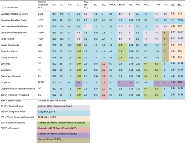
The type of vegetation burned at each fire pixel is determined by the MODIS Col-lection 5 Land Cover Type (LCT) product for 2005 (Friedl et al., 2010). The IGBP land cover classification (Table 1) is used to assign each fire pixel to one of 16 land cover/land use (LULC) classes. Additionally, at each fire point, the MODIS Vegetation Continuous Fields (VCF) product (Collection 3 for 2001) is used to identify the density
15
of the vegetation at each active fire location. The VCF product identifies the percent tree, non-tree vegetation, and bare cover at 500 m resolution (Hansen et al., 2003; Hansen et al., 2005; Carroll et al., 2011). The VCF data are scaled to 1 km spatial resolution to match the fire detection and LCT datasets.
Inconsistencies between the datasets described above are resolved as follows. Any
20
fire detections in areas with the LCT classification for water, snow, or ice are removed (<0.2% of original annual fire points). When the total cover from the VCF product for any fire point does fully cover each pixel, the values are scaled to 100%. This primarily happens as a result of the scaling of the VCF product from 500 m to 1 km resolution. Those fire detections that fall in areas that are 100% bare cover or unclassified
ac-25
GMDD
3, 2439–2476, 2010The Fire INventory from NCAR (FINN)
C. Wiedinmyer et al.
Title Page
Abstract Introduction
Conclusions References
Tables Figures
◭ ◮
◭ ◮
Back Close
Full Screen / Esc
Printer-friendly Version Interactive Discussion
Discussion
P
a
per
|
Dis
cussion
P
a
per
|
Discussion
P
a
per
|
Discussio
n
P
a
per
|
percent cover is reassigned to 50% tree cover and 50% herbaceous cover. For fires in LCT grassland classifications that do not have associated VCF cover information, the percent vegetative cover is reassigned to 20% tree cover and 80% herbaceous cover.
Fire points assigned by the LCT product as “urban” or “bare/sparsely vegetated” are assumed to be open vegetation burning and are reassigned a land cover type based
5
on the total tree and non-tree vegetation cover, as determined by the VCF product. For those fire points with less than 40% tree cover, the urban or sparsely vegetated land cover is reassigned to grasslands; for 40–60% tree cover, the point is reassigned as shrublands; and for tree cover greater than 60% tree cover, the point is reassigned as a forest.
10
The global LULC classifications of the MODIS LCT product are then further lumped into more generic land cover classifications that better match available information on global fuel loadings and emission factors. These generic categories include Savanna and Grasslands (SG), Woody Savannas and Shrublands (WS), Tropical Forest (TROP), Temperate Forest (TEMP), Boreal Forest (BOR), and Cropland (CROP) (Table 1). The
15
evergreen, deciduous, and mixed forest land covers of the LCT are assigned as either boreal or temperate forest depending on the latitude of the point: if latitude is greater than 50◦N, the forest is labeled as a boreal forest.
At present, FINNv1 does not obtain the area burned at each identified fire pixel from burned area products since they are not rapidly available. Therefore, an upper limit
20
is assumed for the burned area. For each fire identified, the assumed burned area is 1 km2, except for fires located in grasslands/savannas: these are assigned a burned area of 0.75 km2 (Wiedinmyer et al., 2006; Al-Saadi et al., 2008). This burned area is further scaled based on the percent bare cover by the VCF product at the fire point. For example, a forest fire detected at a point is assigned a burned area of 1 km2; yet, if
25
that same pixel is assigned 50% bare cover by the VCF dataset, the assigned burned area is 0.5 km2.
GMDD
3, 2439–2476, 2010The Fire INventory from NCAR (FINN)
C. Wiedinmyer et al.
Title Page
Abstract Introduction
Conclusions References
Tables Figures
◭ ◮
◭ ◮
Back Close
Full Screen / Esc
Printer-friendly Version Interactive Discussion
Discussion
P
a
per
|
Dis
cussion
P
a
per
|
Discussion
P
a
per
|
Discussio
n
P
a
per
|
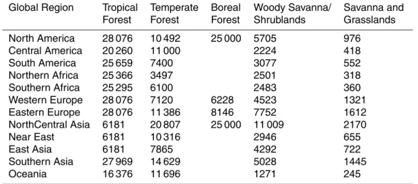
Table 2 of Hoelzemann et al. (2004) and updates shown in our Table 2. For most classes and regions, the average of the GWEM v1.2 and v1.21 are used (Hoelzemann et al., 2004). Changes to the original values presented by Hoelzemann et al. (2004) include the following: (1) Temperate forests in Oceana are assigned the average of the fuel loadings for temperate and tropical forests assigned by Hoelzemann et al. (2004)
5
for that region. (2) The temperate forest loading for Australia, particularly in the euca-lyptus forests of southeastern Australia, is typically much higher than the 7000 g m−2
assigned by Hoelzemann et al. (2004) (C. Murphy, personal communication, 2009) and is been replaced with a larger value. (3) The fuel loading assigned to croplands is 500 g m−2for fires assigned to croplands (Wiedinmyer et al., 2006). The one exception
10
to this rule is for croplands within Brazil, from latitude 20.36◦ to 22.71◦S and longitude
−47.32◦and−49.16◦W. In this region, sugar cane is assumed to be the crop type that
is burned, and the fuel loading here is assigned as 1100 g m−2 (Macedo et al., 2008;
E. Campbell, personal communication, June 2010). This is just one example of how the model can be modified at regional and local levels to include specific information.
15
The fraction of the biomass assumed to burn (FB) at each fire point is assigned as a function of tree cover, as described by Wiedinmyer et al. (2006) and taken from Ito and Penner (2004). For areas with 60% or more tree cover, as defined by the MODIS VCF product, FB is 0.3 for the woody fuel and 0.9 for the herbaceous cover. For areas with less than 40% tree cover, no woody fuel is assumed to burn and the FB is 0.98
20
for the herbaceous cover. Note that these are the upper limits as presented by Ito and Penner (2004). For those fires with 40–60% tree cover, FB is 0.3 for the woody fuels, and FB for the herbaceous fuel is calculated as:
FBherbaceous fuel=e−0
.13×fraction tree cover (2)
The amount of woody fuel available to burn at each fire is determined by the fraction
25
GMDD
3, 2439–2476, 2010The Fire INventory from NCAR (FINN)
C. Wiedinmyer et al.
Title Page
Abstract Introduction
Conclusions References
Tables Figures
◭ ◮
◭ ◮
Back Close
Full Screen / Esc
Printer-friendly Version Interactive Discussion
Discussion
P
a
per
|
Dis
cussion
P
a
per
|
Discussion
P
a
per
|
Discussio
n
P
a
per
|
by the fraction burned and the fractional cover of each vegetation cover (by the MODIS VCF) for each pixel.
For each LULC type, the emission factors for various gaseous and particulate species have been taken from available datasets (see Table 1 and references therein). Detailed emission factors for individual NMOCs emitted by open burning have been
5
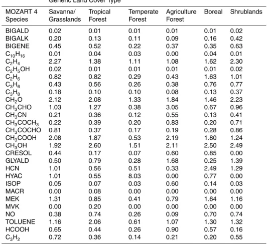
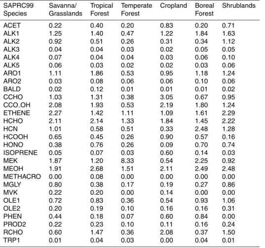
compiled by Akagi et al. (2010), Andreae and Merlet (2001), and (M. O. Andreae, per-sonal communication, October 2008). However, to simulate NMOC chemistry in many models, particularly chemical transport models, many of the individual chemical com-pounds are assigned to “lumped” species in a simplified chemical mechanism. FINNv1 calculates both the total NMOC for each generic land cover type, and also lumps the
10
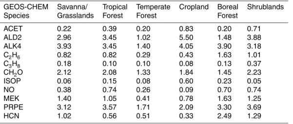
total NMOC emissions as appropriate for various chemical mechanisms. Tables 3–5 include speciation factors developed from the species-specific emissions factors pro-vided by Akagi et al. (2010), Andreae and Merlet (2001), McMeeking (2008), and (M. O. Andreae, personal communication, October 2008). Multiplying the total NMOC emissions (kg) from FINNv1 by the speciation factors shown in the Tables will
pro-15
vide the moles emitted of individual organic compounds or lumped species for the indi-cated chemical mechanism. Here we provide speciation profiles for the GEOS-Chem (Bey et al., 2001; http://www.geos-chem.org/), MOZART-4 (Emmons et al., 2010a), and SAPRC99 (Carter et al., 2000) chemical mechanisms. These speciation profiles are available for use not only with FINNv1 emission estimates, but also other NMOC
20
emission estimates from other models.
The primary differences in the methods described here, compared to the framework presented by Wiedinmyer et al. (2006), include the extension of the model domain from North and Central America to the globe; the removal of fire detections with con-fidence less than 20%; the “smoothing” of the fire detections in the tropical latitudes
25
GMDD
3, 2439–2476, 2010The Fire INventory from NCAR (FINN)
C. Wiedinmyer et al.
Title Page
Abstract Introduction
Conclusions References
Tables Figures
◭ ◮
◭ ◮
Back Close
Full Screen / Esc
Printer-friendly Version Interactive Discussion
Discussion
P
a
per
|
Dis
cussion
P
a
per
|
Discussion
P
a
per
|
Discussio
n
P
a
per
|
significant differences between the results obtained from earlier versions of this model framework (e.g., Wiedinmyer at al., 2006; Wiedinmyer and Neff, 2007).
3 Results
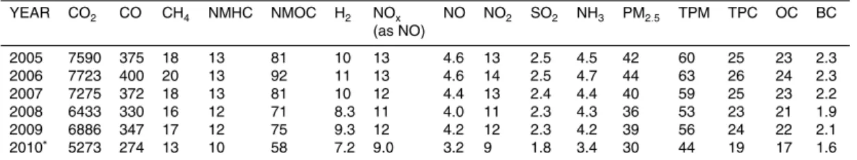
Daily fire emissions for 1 January 2005 through 27 August 2010 were estimated using the FINNv1 model framework and inputs described here. The daily global results for
5
the MOZART-4 and SAPRC99 chemical mechanisms are available for download and use at http://bai.acd.ucar.edu/Data/fire/. The global total emissions of key trace gases and particulate species for each year from 2005–2009 and 2010 through 27 August are shown in Table 6.
3.1 Comparison of FINNv1 to other biomass burning inventories
10
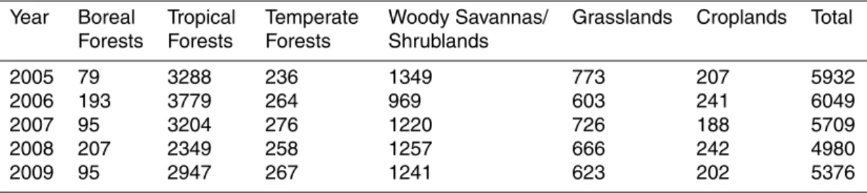
On a global scale, the biomass consumption and total emissions predicted with FINNv1 are fairly similar to amounts from other global estimates. For example, the total global biomass burned in GICC (Mieville et al., 2010) for 2000 was estimated to be 5790 Tg, and the average annual global biomass burned from 2005–2009 estimated with FINNv1 is 5609 Tg (Table 7). The global annual FINNv1 CO2emission estimates
15
are∼5–30% larger than the GFEDv3.1 estimates (Table 8). The agreement is
vari-able by year and the differences result primarily from the different fuel consumption approaches that drive the two models.
Next we compare the detailed emissions of various, mostly reactive, species. For 2005, the GICC estimates 504 Tg CO, 20.5 Tg NOx (as NO2), and 3.8 Tg BC for 2005.
20
FINNv1 estimates for these compounds for 2005 are 375 Tg CO, 20.4 Tg NOx(as NO2), and 2.3 Tg BC. The average annual PM2.5 estimate from FINNv1 (2006–2008) was
40 Tg, whereas this number was 44 Tg from GFEDv2 and 110 Tg from FLAMBE (Reid et al., 2009). The different estimates for the above species are consistent within the uncertainties of the model frameworks (see Sect. 3.5).
GMDD
3, 2439–2476, 2010The Fire INventory from NCAR (FINN)
C. Wiedinmyer et al.
Title Page
Abstract Introduction
Conclusions References
Tables Figures
◭ ◮
◭ ◮
Back Close
Full Screen / Esc
Printer-friendly Version Interactive Discussion
Discussion
P
a
per
|
Dis
cussion
P
a
per
|
Discussion
P
a
per
|
Discussio
n
P
a
per
|
The organic compounds emitted by fires are reactive species that play a role in the formation of ozone and secondary organic aerosol. Thus, accurate estimates of the organic emissions from open burning are critical input for any atmospheric chemistry or air quality model. Comparison of organic emissions derived from FINNv1 with pre-vious BB estimates or with other sources of organic emissions (Sect. 3.2) requires
5
clarification of the relevant terminology, which is also discussed in more detail in Akagi et al. (2010). Non-methane hydrocarbons (NMHC) are organic molecules that by def-inition contain only atoms of C and H such as alkenes and alkanes. In early biomass burning research, NMHC were thought to account for nearly all the organic compounds emitted by fires and it became commonplace to equate NMHC emissions to total
or-10
ganic emissions. More recent work has shown that 60–80% of the identifiable organic compounds emitted by fires contain oxygen atoms in addition to C and H (Yokelson et al., 1996, 2008; Holzinger et al., 1999; Karl et al., 2007). A broader term for or-ganic emissions that includes the oxygenated oror-ganic compounds (e.g. formaldehyde, methanol, etc.) is non-methane organic compounds (NMOC). An updated
compila-15
tion of EF for NMOC by Akagi et al. (2010) is incorporated into FINNv1. However, in some other estimates the term NMHC is still used and the quantity represented by this term may vary. Sometimes NMHC refers to just the molecules with C and H (van der Werf et al., 2006, 2010). In other studies, the term NMHC is not defined and thus un-clear, but it may be intended to indicate the NMHC plus the other NMOC. In any case,
20
the intent of previous work was probably to estimate total organic emissions regard-less of the terminology. Here we compare the amount of identified NMOC emitted by open burning, as derived by FINNv1, to previous estimates of total organic emissions. One other clarification is worthwhile. In studies that measure fire emissions by mass spectrometry or gas chromatography only about one-half of the NMOC peaks can be
25
GMDD
3, 2439–2476, 2010The Fire INventory from NCAR (FINN)
C. Wiedinmyer et al.
Title Page
Abstract Introduction
Conclusions References
Tables Figures
◭ ◮
◭ ◮
Back Close
Full Screen / Esc
Printer-friendly Version Interactive Discussion
Discussion
P
a
per
|
Dis
cussion
P
a
per
|
Discussion
P
a
per
|
Discussio
n
P
a
per
|
however, estimates of total global NMOC that include the unidentified species can be found in Akagi et al. (2010). The emissions of NMOC from FINNv1 are a factor of 3.7 to 4.9 higher than the GFEDv3 NMHC emission estimates, as is to be expected due to the consideration of more species of organic emissions in FINNv1 (Table 8).
3.2 Comparison of biomass burning to other sources
5
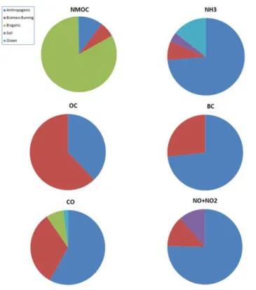
The open biomass burning emissions from FINNv1 for 2008 make up 27% of global particulate BC emissions, 33% of global CO emissions, and 62% of global primary particulate OC emissions; where the 2008 global totals were estimated by Emmons et al. (2010a) (Fig. 1).
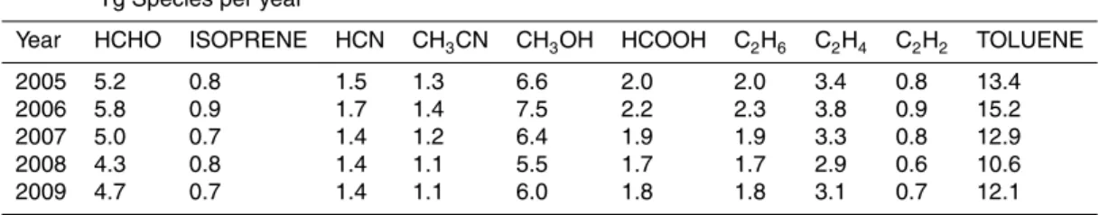
Emissions of individual organic species are estimated from the total global NMOC
10
emissions using the speciation profiles presented in Tables 3 through 5. The global annual totals of a few key organic compounds calculated with the MOZART-4 and SAPRC99 speciation profiles are shown in Table 9. Isoprene, the most abundant bio-genic emission, is also emitted by open fires, but in small amounts compared to the 600 Tg emitted from undisturbed vegetation (Guenther et al., 2006). However, the fire
15
emissions of other individual NMOC species can be more important. Globally, the av-erage annual methanol (CH3OH) emissions from open biomass burning are 2.8 times larger than the anthropogenic emissions of CH3OH, and the emissions of formalde-hyde (CH2O) are a factor of 1.4 larger than anthropogenic emissions (Emmons et al.,
2010a). Note that that the above ratios compare open biomass burning to other
es-20
timates of anthropogenic emissions, and biofuel use (primarily cooking with biomass fuel) is included in the anthropogenic category.
3.3 High variability and major features of emission rates
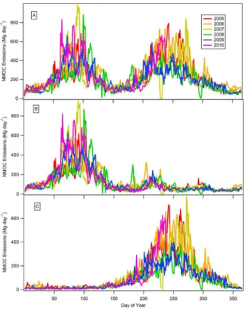
The daily emissions of total identified NMOC for the Northern Hemisphere, the South-ern Hemisphere, and the globe are shown in Fig. 2. The interannual variability can be
25
GMDD
3, 2439–2476, 2010The Fire INventory from NCAR (FINN)
C. Wiedinmyer et al.
Title Page
Abstract Introduction
Conclusions References
Tables Figures
◭ ◮
◭ ◮
Back Close
Full Screen / Esc
Printer-friendly Version Interactive Discussion
Discussion
P
a
per
|
Dis
cussion
P
a
per
|
Discussion
P
a
per
|
Discussio
n
P
a
per
|
emissions for specific time periods can vary by more than a factor of two from year to year. The NMOC emissions (as well as the other emissions of other species not shown) are also extremely variable day to day confirming the need for high temporal resolution for some applications.
The major temporal features of the FINNv1 emissions are summarized next. Two
5
general peaks in emissions occur each year. The first peak is from∼ mid-February
through May and is primarily caused by the burning in the tropical and subtropical regions of the Northern Hemisphere. A second peak occurs from August through September, which corresponds to burning in the Southern Hemisphere tropics. As-suming that CO2 and NMOC are emitted proportionally from open biomass burning,
10
this second peak in emissions is qualitatively similar to what is presented for open burning CO2 emissions estimated by the GICC. However, the first peak in FINNv1
NMOC emissions is somewhat different from the GICC CO2estimates for 1997–2005,
which show a peak in the global CO2emissions starting in January of each year (Fig. 4 of Mieville et al., 2010).
15
Regionally, emissions from open biomass burning show substantial variability. Fig-ure 3 shows the spatial distribution of CO emissions from FINNv1 (allocated to a 1◦
×1◦
resolution) for four months (January, April, July, and October) in 2008. FINNv1 emis-sions for January are relatively low and are centered near the equator. CO emisemis-sions in the tropical Northern Hemisphere, specifically Southeast Asia and Central America,
20
are high during the spring months. There are also large emissions associated with burning throughout Central Asia. SH emission predicted for July are located mainly in South America and Africa, while NH July emissions are found mainly in North Amer-ica, and Northern Asia. In October, open burning emissions are mostly produced in the Southern Hemisphere (Fig. 2)
25
3.4 Applications
GMDD
3, 2439–2476, 2010The Fire INventory from NCAR (FINN)
C. Wiedinmyer et al.
Title Page
Abstract Introduction
Conclusions References
Tables Figures
◭ ◮
◭ ◮
Back Close
Full Screen / Esc
Printer-friendly Version Interactive Discussion
Discussion
P
a
per
|
Dis
cussion
P
a
per
|
Discussion
P
a
per
|
Discussio
n
P
a
per
|
emissions or their predecessors have already been used successfully in several re-gional and global applications (e.g., Fast et al., 2009; Emmons et al., 2010b; Pfister et al., 2008; Hodzic et al., 2008). Methods for allocating the emissions to a diurnal cycle and incorporating plume rise can be found elsewhere (e.g., Frietas et al., 2009; WRAP, 2005). Because the FINNv1 emissions can be produced within a few hours
5
of each satellite overpass, they can be used for model forecast applications. FINNv1 emissions can be generated interactively and feedback provided by users will improve future versions of the model. The FINNv1 emission estimates have advantages over some other inventories when high spatial and/or temporal resolution or rapid availabil-ity is needed. For example, despite the limitations of using the daily fire counts (see
10
Sect. 3.5), the daily estimates allow models to capture the highly episodic nature of fire emissions that could be missed with smoothing to 8-day resolution or using monthly fire counts, as is commonly done. Additionally, FINNv1 produces consistent emission estimates from coarse grid scales to local scales, which facilitates comparisons and is useful for nested applications.
15
3.5 Limitations and uncertainties
FINNv1 produces high-resolution (spatial and temporal) emissions from open biomass burning on a global scale relatively quickly (on the order of minutes to hours). Although useful for multiple applications, the estimates are very uncertain and have only begun to be compared to observations (e.g., Pfister et al., 2010). Uncertainties associated
20
with many aspects of the estimation process are described in detail by Wiedinmyer et al. (2006) and below. In summary, since most global fires are “small” it is likely that the largest uncertainties arise from (1) missed fires causing an underestimation of the number of fires and (2) overestimating the size of the small fires that are detected. These errors tend to cancel as discussed by Wiedinmyer et al. (2006) and Yokelson et
25
GMDD
3, 2439–2476, 2010The Fire INventory from NCAR (FINN)
C. Wiedinmyer et al.
Title Page
Abstract Introduction
Conclusions References
Tables Figures
◭ ◮
◭ ◮
Back Close
Full Screen / Esc
Printer-friendly Version Interactive Discussion
Discussion
P
a
per
|
Dis
cussion
P
a
per
|
Discussion
P
a
per
|
Discussio
n
P
a
per
|
assumptions made in FINNv1 also add uncertainty, such as the smoothing of the fire detections in tropical latitudes to account for the lack of daily coverage by the MODIS instruments in this region, and the assumed burned area of each fire. For the global ap-plication described here, average values for variable phenomena are applied to broad regions. The average value may not always represent the real value for some fires or
5
some years. Next we discuss three of the sources of uncertainty in more detail. Satellite overpass timing and cloud cover may prevent the detection of fires. The need to estimate the number of fires on days without coverage limits the accuracy of any emissions model. Additionally, all remote sensing thermal anomaly products do not detect most of the fires less than∼100 ha and some understory fires (e.g. Hawbaker
10
et al., 2008), both of which can be a significant source of emissions to the atmosphere. The land use/land cover (LULC) classifications assigned to the fires introduces some uncertainty to the emission estimates. For the results presented here, the satellite-derived MODIS LCT and VCF products are used to identify the type and density of vegetation burned. These products were chosen specifically because of their
consis-15
tency with the MODIS fire detections, easy access, and easy use. Yet, determination of ecosystem type can vary significantly from one land cover data product to another. For example, Wiedinmyer et al. (2006) showed that the use of three different LULC datasets to drive a regional fire emissions model for North and Central America led to 26% differences in annual emission estimates. Those authors ultimately selected the
20
Global Land Cover 2000 product (GLC2000; Fritz et al., 2003) to determine the land cover burned at each fire in North and Central America (Wiedinmyer et al., 2006). Giri et al. (2005) detail differences in the MODIS LCT product and the GLC2000 dataset and show that the area totals of the generic land covers agree reasonable well glob-ally, except for woody savannas/shrublands and wetlands. However, at the pixel level,
25
GMDD
3, 2439–2476, 2010The Fire INventory from NCAR (FINN)
C. Wiedinmyer et al.
Title Page
Abstract Introduction
Conclusions References
Tables Figures
◭ ◮
◭ ◮
Back Close
Full Screen / Esc
Printer-friendly Version Interactive Discussion
Discussion
P
a
per
|
Dis
cussion
P
a
per
|
Discussion
P
a
per
|
Discussio
n
P
a
per
|
Correct assignment of the vegetation does not prevent uncertainty due to the fuel consumption estimates. For instance, only one value for fuel loading is assigned to each land cover type in each region. A constant value is most likely not representative of a vegetation class within an entire region and will not reproduce the full heterogene-ity of the landscapes. For example, Soja et al. (2004) found that disparities in the
5
amount of carbon stored in unique Siberian ecosystems and the severity of fire events can affect total direct carbon emissions by as much as 50%. However, a strength of FINNv1 is that it is relatively easy to introduce specific regional information to replace the generic information in an effort to reduce uncertainties in the emission estimation process. For example, as discussed above, specific fuel loadings for crop fires in a
10
small area of Brazil were applied to account for sugar cane burning.
The uncertainty in total emissions that can arise from coupling all the inherent un-certainties is illustrated briefly with a few examples. Al-Saadi et al. (2009) reported that monthly fire emission estimates generated for the contiguous US over several months in 2006 by various remote sensing-based techniques varied by an order of
15
magnitude. Chang and Song (2010) used two different burned area products to de-rive their open burning emissions for Southeast Asia: the L3JRC and the Collection 5 MODIS (MCD45A1) burned-area products. They found that the average annual burned area estimates for the two products over Asia from 2000–2006 were almost a factor of 2 different, and the interannual variation in the burned area estimates differed as well.
20
When compared to the annual average burned area estimates of GFEDv2 for the same time period, GFEDv2 was 50% greater than the MCD45A1 burned area estimates and almost a factor of 2 higher than the L3JRC estimates.
In light of the above discussion, we examine some of the sources of uncertainty in FINNv1 in more detail. For a sensitivity test, we used the GLOBCOVER global
25
GMDD
3, 2439–2476, 2010The Fire INventory from NCAR (FINN)
C. Wiedinmyer et al.
Title Page
Abstract Introduction
Conclusions References
Tables Figures
◭ ◮
◭ ◮
Back Close
Full Screen / Esc
Printer-friendly Version Interactive Discussion
Discussion
P
a
per
|
Dis
cussion
P
a
per
|
Discussion
P
a
per
|
Discussio
n
P
a
per
|
However, the amount of some landcover types that is assumed to burn globally in each run changes substantially when the different land cover datasets are applied, which can have large impacts on the estimated emissions from a region since different land covers have varying emission factors and fuel loadings that can lead to variations in emission estimates. For example, globally for 2006, the GLOBCOVER simulation
es-5
timates that more than 3 times the amount of temperate forest burns compared to the default run driven by the MODIS LCT data. Additionally, the LCT data implies that more shrubland and grasslands burn globally. Regionally variation is also high. For example, the GLOBCOVER assigned 70% more forest fires to the contiguous US, Mexico, and Central America, leading to 20% higher CO and 24% higher NMOC emissions than
10
the default simulation in these regions. In this case, the MODIS LCT assigned more shrubland, cropland and grassland fires. The total emissions estimated using GLOB-COVER were only 10% lower in Canada and Alaska than the default simulation, due to fewer forest fires assigned in these areas.
In summary, a quantitative assignment of uncertainty is difficult, due to the
uncer-15
tainties associated with the land cover classifications, the fire detections, the assumed area burned, the biomass loading, the amount of fuel burned, and emission factors. At this time, we follow other efforts (e.g., Wiedinmyer et al., 2006; Mieville et al., 2010) and assign the uncertainty as a factor of two for the FINNv1 estimates. We continue to apply in situ measurements, satellite observations, and model simulations to
evalu-20
ate the accuracy of the estimates provided here. Future versions of FINN will contain updates intended to reduce these uncertainties.
4 Conclusions
Open biomass burning injects significant amounts of particulate matter and trace gases into the atmosphere. The Fire INventory from NCAR version 1.0 (FINNv1) estimates
25
GMDD
3, 2439–2476, 2010The Fire INventory from NCAR (FINN)
C. Wiedinmyer et al.
Title Page
Abstract Introduction
Conclusions References
Tables Figures
◭ ◮
◭ ◮
Back Close
Full Screen / Esc
Printer-friendly Version Interactive Discussion
Discussion
P
a
per
|
Dis
cussion
P
a
per
|
Discussion
P
a
per
|
Discussio
n
P
a
per
|
also provides speciation profiles for several lumped chemical mechanisms used by some chemical transport models. FINNv1 includes updated emission factors for non-methane organic compounds, which may have an important impact on the way in which global and regional chemistry is simulated. Strengths of FINNv1 include: it quickly provides modelers with reasonable, high temporal/spatial resolution fire emission
esti-5
mates based on updated emission factors, and it is easily adapted to more accurately target specific regions of interest.
For many chemical species, the FINNv1 emission estimates agree well with other inventories; specifically the GICC and the GFEDv3. However, this does not in itself establish the absolute accuracy of the estimates because open burning emission
esti-10
mates are subject to inherent limitations that lead to large uncertainties. Thus, the un-certainty assigned to the FINNv1 estimates is a factor of 2. Future work will compare the FINNv1 estimates to in situ measurements, satellite observations, and chemical transport models.
Acknowledgements. The National Center for Atmospheric Research is operated by the
Univer-15
sity Corporation for Atmospheric Research under sponsorship of the National Science Founda-tion. The authors greatly thank Minnie Wong of the University of Maryland for the distribution of the MODIS fire count data. CW thanks Matthew Evans for assistance with the GEOS-chem mechanism.
References
20
Akagi, S. K., Yokelson, R. J., Wiedinmyer, C., Alvarado, M. J., Reid, J. S., Karl, T., Crounse, J. D., and Wennberg, P. O.: Emission factors for open and domestic biomass burning for use in atmospheric models, Atmos. Chem. Phys. Discuss., 10, 27523–27602, doi:10.5194/acpd-10-27523-2010, 2010.
Al-Saadi, J. A., Soja, A. J., Pierce, R. B., Szykman, J., Wiedinmyer, C., Emmons, L. K.,
Kon-25
GMDD
3, 2439–2476, 2010The Fire INventory from NCAR (FINN)
C. Wiedinmyer et al.
Title Page
Abstract Introduction
Conclusions References
Tables Figures
◭ ◮
◭ ◮
Back Close
Full Screen / Esc
Printer-friendly Version Interactive Discussion
Discussion
P
a
per
|
Dis
cussion
P
a
per
|
Discussion
P
a
per
|
Discussio
n
P
a
per
|
Andreae, M. O. and Merlet, P.: Emission of trace gases and aerosols from biomass burning, Global Biogeochem. Cy., 15(4), 955–966, 2001.
Andreae, M. O. and Rosenfeld, D.: Aerosol-cloud-precipitation interactions. Part 1. The nature and sources of cloud-active aerosols. Earth Sci. Rev., 89, 13–41, doi:10.1016/j.earscirev.2008.03.001, 2008.
5
Arellano, A. F., Kasibhatla, P. S., Giglio, L., van der Werf, G. R., and Randerson, J. T.: Top-down estimates of global CO sources using MOPITT measurements, Geophys. Res. Lett., 31, L01104, doi:10.1029/2003GL018609, 2004.
Arellano, A. F., Jr., Kasibhatla, P. S., Giglio, L., van der Werf, G. R., Randerson, J. T., and Collatz, G. J.: Time- dependent inversion estimates of global biomass-burning CO emissions
10
using Measurement of Pollution in the Troposphere (MOPITT) measurements, J. Geophys. Res., 111, D09303, doi:10.1029/2005JD006613, 2006.
Bey, I., Jacob, D. J., Yantosca, R. M., Logan, J. A., Field, B., Fiore, A. M., Li, Q., Liu, H., Mickley, L. J., and Schultz, M.: Global modeling of tropospheric chemistry with assimilated meteorology: Model description and evaluation, J. Geophys. Res., 106, 23073–23096, 2001.
15
Bond, T. C., Streets, D. G., Yarber, K. F., Nelson, S. M., Woo, J.-H., and Klimont, Z.: A technology-based global inventory of black and organic carbon emissions from combustion, J. Geophys. Res., 109, D14203, doi:10.1029/2003JD003697, 2004.
Campbell, J., Donato, D., Azuma, D., and Law, B.: Pyrogenic carbon emission from a large wild-fire in Oregon, United States, J. Geophys. Res., 112, G04014, doi:10.1029/2007JG000451,
20
2007.
Carroll, M., Townshend, J., Hansen, M., DiMiceli, C., Sohlberg, R., and Wurster, K.: Vegetative Cover Conversion and Vegetation Continuous Fields, in: Land Remote Sensing and Global Environmental Change: NASA’s Earth Observing System and the Science of Aster and MODIS Springer-Verlag, edited by: Ramachandran, B., Justice, C. O., Abrams, M., in press,
25
2010.
Carter, W. P. L.: Implementation of the SAPRC-99 chemical mechanism into the Models-3 framework, U.S. EPA, 2000.
Chang, D. and Song, Y.: Estimates of biomass burning emissions in tropical Asia based on satellite-derived data, Atmos. Chem. Phys., 10, 2335–2351, doi:10.5194/acp-10-2335-2010,
30
2010.
GMDD
3, 2439–2476, 2010The Fire INventory from NCAR (FINN)
C. Wiedinmyer et al.
Title Page
Abstract Introduction
Conclusions References
Tables Figures
◭ ◮
◭ ◮
Back Close
Full Screen / Esc
Printer-friendly Version Interactive Discussion
Discussion
P
a
per
|
Dis
cussion
P
a
per
|
Discussion
P
a
per
|
Discussio
n
P
a
per
|
emissions: 1. Emissions from Indonesian, African, and other fuels, J. Geophys. Res., 108, 4719, doi:10.1029/2003JD003704, 2003.
Colarco, P., da Silva, A., Chin, M., and Diehl, T.: Online simulations of global aerosol distribu-tions in the NASA GEOS-4 model and comparisons to satellite and ground-based aerosol optical depth, J. Geophys. Res., 115, D14207, doi:10.1029/2009JD012820, 2010.
5
Crutzen, P. J. and Andeae, M. O.: Biomass burning in the tropics- impact on atmospheric chemistry and biogeochemical cycles, Science, 250, 4988, 1669–1678, 1990.
Davies, D. K., Ilavajhala, S., Wong, M. M., and Justice, C. O.: Fire Information for Resource Management System: Archiving and Distributing MODIS Active Fire Data, IEEE T. Geosci. Remote Sens., 47(1), 72–79, 2009.
10
Duncan, B. N., Martin, R. V., Staudt, A. C., Yevich, R., and Logan, J. A.: Interannual and seasonal variability of biomass burning emissions constrained by satellite observations, J. Geophys. Res., 108(D2), 4100, doi:10.1029/2002JD002378, 2003.
Friedl, M. A., Sulla-Menashe, D., Tan, B., Schneider, A., Ramankutty, N., Sibley, A., and Huang, X.: MODIS collection 5 global land cover: algorithm refinements and characterization of new
15
datasets, Remote Sens. Environ., 114(1), 168–182, 2010.
Emmons, L. K., Walters, S., Hess, P. G., Lamarque, J.-F., Pfister, G. G., Fillmore, D., Granier, C., Guenther, A., Kinnison, D., Laepple, T., Orlando, J. J., Tie, X., Tyndall, G., Wiedin-myer, C., Baughcum, S. L., and Kloster, S.: Description and evaluation of the Model for Ozone and Related chemical Tracers, version 4 (MOZART-4), Geosci. Model Dev., 3, 43–67,
20
doi:10.5194/gmd-3-43-2010, 2010a.
Emmons, L. K., Apel, E. C., Lamarque, J.-F., Hess, P. G., Avery, M., Blake, D., Brune, W., Cam-pos, T., Crawford, J., DeCarlo, P. F., Hall, S., Heikes, B., Holloway, J., Jimenez, J. L., Knapp, D. J., Kok, G., Mena-Carrasco, M., Olson, J., O’Sullivan, D., Sachse, G., Walega, J., Weib-ring, P., Weinheimer, A., and Wiedinmyer, C.: Impact of Mexico City emissions on regional air
25
quality from MOZART-4 simulations, Atmos. Chem. Phys., 10, 6195–6212, doi:10.5194/acp-10-6195-2010, 2010b.
Fast, J., Aiken, A. C., Allan, J., Alexander, L., Campos, T., Canagaratna, M. R., Chapman, E., DeCarlo, P. F., de Foy, B., Gaffney, J., de Gouw, J., Doran, J. C., Emmons, L. K., Hodzic, A., Herndon, S. C., Huey, G., Jayne, J. T., Jimenez, J. L., Kleinman, L., Kuster, W., Marley,
30
GMDD
3, 2439–2476, 2010The Fire INventory from NCAR (FINN)
C. Wiedinmyer et al.
Title Page
Abstract Introduction
Conclusions References
Tables Figures
◭ ◮
◭ ◮
Back Close
Full Screen / Esc
Printer-friendly Version Interactive Discussion
Discussion
P
a
per
|
Dis
cussion
P
a
per
|
Discussion
P
a
per
|
Discussio
n
P
a
per
|
implications for assessing treatments of secondary organic aerosols, Atmos. Chem. Phys., 9, 6191–6215, doi:10.5194/acp-9-6191-2009, 2009.
Freitas, S. R., Longo, K. M., Silva Dias, M. A. F., Chatfield, R., Silva Dias, P., Artaxo, P., Andreae, M. O., Grell, G., Rodrigues, L. F., Fazenda, A., and Panetta, J.: The Coupled Aerosol and Tracer Transport model to the Brazilian developments on the Regional Atmospheric Modeling
5
System (CATT-BRAMS) – Part 1: Model description and evaluation, Atmos. Chem. Phys., 9, 2843-2861, doi:10.5194/acp-9-2843-2009, 2009.
Fritz, S., Bartholom ´e, E., Belward, A., Hartley, A., Stibig, H.-J., Eva, H., Mayaux, P., Bartalev, S., Latifovic, R., Kolmert, S., Roy, P., Agrawal, S., Bingfang,W., Wenting, X., Ledwith, M., Pekel, F. J., Giri, C., M ¨ucher, S., Badts, E., Tateishi, R., Champeaux, J.-L., and Defourny, P.:
10
Harmonization, mosaicing, and production of the Global Land Cover 2000 database (Beta Version), Ispra, Italy Joint Research Center (JRC), 2003.
Giglio, L., Csiszar, I., and Justice, C. O.: Global distribution and seasonality of active fires as observed with the Terra and Aqua Moderate Resolution Imaging Spectroradiometer (MODIS) sensors, J. Geophys. Res., 111, G02016, doi:10.1029/2005JG000142, 2006.
15
Giglio, L., Randerson, J. T., van der Werf, G. R., Kasibhatla, P. S., Collatz, G. J., Morton, D. C., and DeFries, R. S.: Assessing variability and long-term trends in burned area by merging multiple satellite fire products, Biogeosciences, 7, 1171–1186, doi:10.5194/bg-7-1171-2010, 2010.
Giri, C., Zhu, Z., and Reed, B.: A comparative analysis of the Global Land Cover 2000 and
20
MODIS land cover data sets, Remote Sens. Environ., 94, 123–132, 2005.
Guenther, A., Karl, T., Harley, P., Wiedinmyer, C., Palmer, P. I., and Geron, C.: Estimates of global terrestrial isoprene emissions using MEGAN (Model of Emissions of Gases and Aerosols from Nature), Atmos. Chem. Phys., 6, 3181–3210, doi:10.5194/acp-6-3181-2006, 2006.
25
Hansen, M. C., DeFries, R. S., Townshend, J. R. G., Carroll, M., DiMiceli, C., and Sohlberg, R.: Global percent tree cover at a spatial resolution of 500 meters: first results of the MODIS Vegetation Continuous Fields algorithm, Earth Interact., 7, 1–15, 2003.
Hansen, M. C., Townshend, J. R. G., DeFries, R. S., and Carroll, M.: Estimation of tree cover using MODIS data at global, continental and regional/local scales, Int. J. Remote Sens., 26,
30
4359–4380, 2005.
GMDD
3, 2439–2476, 2010The Fire INventory from NCAR (FINN)
C. Wiedinmyer et al.
Title Page
Abstract Introduction
Conclusions References
Tables Figures
◭ ◮
◭ ◮
Back Close
Full Screen / Esc
Printer-friendly Version Interactive Discussion
Discussion
P
a
per
|
Dis
cussion
P
a
per
|
Discussion
P
a
per
|
Discussio
n
P
a
per
|
2656–2664, 2008.
Hodzic, A., Madronich, S., Bohn, B., Massie, S., Menut, L., and Wiedinmyer, C.: Wildfire par-ticulate matter in Europe during summer 2003: meso-scale modeling of smoke emissions, transport and radiative effects, Atmos. Chem. Phys., 7, 4043–4064, doi:10.5194/acp-7-4043-2007, 2007.
5
Hoelzemann, J. J., Schultz, M. G., Brasseur, G. P., Granier, C., and Simon, M.: Global Wild-land Fire Emission Model (GWEM): Evaluating the use of global area burnt satellite data, J. Geophys. Res., 109, D14S04, doi:10.1029/2003JD003666, 2004.
Holzinger, R., Warneke, C., Hansel, A., Jordan, A., Lindinger, W., Scharffe, D. H., Schade, G., and Crutzen, P. J.: Biomass burning as a source of formaldehyde, acetaldehyde, methanol,
10
acetone, acetonitrile, and hydrogen cyanide, Geophys. Res. Lett., 26(8), 1161–1164, 1999. IPCC: in: Contribution of Working Group I to the Fourth Assessment Report of the
Intergov-ernmental Panel on Climate Change, edited by: Solomon, S., Qin, D., Manning, M., Chen, Z., Marquis, M., Averyt, K. B., Tignor, M., and Miller, H. L., Cambridge University Press, Cambridge, United Kingdom and New York, NY, USA, 2007.
15
Ito, A. and Penner, J. E.: Global estimates of biomass burning emissions based on satellite imagery for the year 2000, J. Geophys. Res., 109, D14S05, doi:10.1029/2003JD004423, 2004.
Karl, T., Guenther, A., Yokelson, R. J., Greenberg, J., Potosnak, M., Blake, D. R., and Artaxo, P.: The tropical forest and fire emissions experiment: Emission, chemistry, and transport of
20
biogenic volatile organic compounds in the lower atmosphere over Amazonia, J. Geophys. Res., 112, D18302, doi:10.1029/2007JD008539, 2007.
Larkin, N. K., O’Neill, S. M., Solomon, R., Raffuse, S., Strand, T., Sullivan, D. C., Krull, C., Rorig, M., Peterson, J. L., and Ferguson, S. A.: The BlueSky smoke modeling framework, Int. J. Wildland Fire, 18(8), 906–920, 2009.
25
Lavoue, D., Liousse, C., Cachier, H., Stocks, B. J., and Goldammer, J. G.: Modeling of carbona-ceous particles emitted by boreal and temperate wildfires at northern latitudes, J. Geophys. Res., 105(D22), 26871–26890, 2000.
Lobert, J. M., Keene, W. C., Logan, J. A., and Yevich, R.: Global chlorine emissions from biomass burning: reactive chlorine emissions inventory, J. Geophys. Res.-Atmos., 104(D7),
30
8373–8389, 1999.
GMDD
3, 2439–2476, 2010The Fire INventory from NCAR (FINN)
C. Wiedinmyer et al.
Title Page
Abstract Introduction
Conclusions References
Tables Figures
◭ ◮
◭ ◮
Back Close
Full Screen / Esc
Printer-friendly Version Interactive Discussion
Discussion
P
a
per
|
Dis
cussion
P
a
per
|
Discussion
P
a
per
|
Discussio
n
P
a
per
|
2020, Biomass Bioenerg., 32(7), 582–595, 2008.
Magi, B. I., Ginoux, P., Ming, Y., and Ramaswamy, V.: Evaluation of tropical and extratropical Southern Hemisphere African aerosol properties simulated by a climate model, J. Geophys. Res., 114, D14204, doi:10.1029/2008JD011128, 2009.
McMeeking, G. R., Kreidenweis, S. M., Lunden, M., Carrillo, J., Carrico, C. M., Lee, T., Herckes,
5
P., Engling, G., Day, D. E., Hand, J., Brown, N., Malm, W. C., and Collett, J. L.: Smoke-impacted regional haze in California during the summer of 2002, Agri. Forest Meteorol., 137(1–2), 25–42, 2006.
McMeeking, G. R.: The optical, chemical, and physical properties of aerosols and gases emit-ted by the laboratory combustion of wildland fuels, Ph.D. Dissertation, Department of
Atmo-10
spheric Sciences, Colorado State University, 109–113, Fall 2008.
Michel, C., Liousse, C., Gr ´egoire, J.-M., Tansey, K., Carmichael, G. R., and Woo, J.-H.: Biomass burning emission inventory from burnt area data given by the SPOT-VEGETATION system in the frame of TRACE-P and ACE-Asia campaigns, J. Geophys. Res., 110, D09304, doi:10.1029/2004JD005461, 2005.
15
Mieville, A., Granier, C., Liousse, C., Guillaume, B., Mouillot, F., Lamarque, F., Gr ´egoire, J.-M., and Petron, G.: Emissions of gases and particles from biomass burning during the 20th century using satellite data and an historical reconstruction, Atmos. Environ., 44, 1469–1477, 2010.
Muhle, J., Lueker, T. J., Su, Y., Miller, B. R., Prather, K. A., and Weiss, R. F.: Trace gas and
20
particulate emissions from the 2003 southern California wildfires, J. Geophys. Res., 112, D03307, doi:10.1029/2006JD007350, 2007.
NASA/University of Maryland, MODIS Hotspot/Active Fire Detections, Data set, MODIS Rapid Response Project, NASA/GSFC [producer], University of Maryland, Fire Information for Resource Management System [distributors], available online http://maps.geog.umd.edu,
25
2002.
Nassar, R., Logan, J. A., Megretskaia, I. A., Murray, L. T., Zhang, L., and Jones, D. B. A.: Anal-ysis of tropical tropospheric ozone, carbon monoxide, and water vapor during the 2006 El Ni ˜no using TES observations and the GEOS-Chem model, J. Geophys. Res., 114, D17304, doi:10.1029/2009JD011760, 2009.
30
GMDD
3, 2439–2476, 2010The Fire INventory from NCAR (FINN)
C. Wiedinmyer et al.
Title Page
Abstract Introduction
Conclusions References
Tables Figures
◭ ◮
◭ ◮
Back Close
Full Screen / Esc
Printer-friendly Version Interactive Discussion
Discussion
P
a
per
|
Dis
cussion
P
a
per
|
Discussion
P
a
per
|
Discussio
n
P
a
per
|
doi:10.1080/15693430500400345, 2005.
Pfister, G. G., Wiedinmyer, C., and Emmons, L. K.: Impacts of the fall 2007 California wildfires on surface ozone: Integrating local observations with global model simulations, Geophys. Res. Lett., 35(19), doi:10.1029/2008GL034747, 2008.
Pfister, G. G., Parrish, D., Worden, H., Emmons, L. K., Edwards, D. P., Wiedinmyer, C., Diskin,
5
G. S., Huey, G., Oltmans, S. J., Thouret, V., Weinheimer, A., and Wisthaler, A.: Characteriz-ing summertime chemical boundary conditions for airmasses enterCharacteriz-ing the US West Coast, Atmos. Chem. Phys. Discuss., 10, 28909–28962, doi:10.5194/acpd-10-28909-2010, 2010. Pope, C. A. and Dockery, D. W.: Health effects of fine particulate air pollution: Lines that
connect, J. Air Waste Ma., 56(6), 709–742, 2006.
10
Randerson, J. T., van der Werf, G. R., Collatz, G. J., Giglio, L., Still, C. J., Kasibhatla, P., Miller, J. B., White, J. W. C., DeFries, R. S., and Kasischke, E. S.: Fire emissions from C3 and C4vegetation and their influence on interannual variability of atmospheric CO2and d13CO2, Global Biogeochem. Cy., 19, GB2019, doi:10.1029/2004GB002366, 2005.
Reid, J. S., Hyer, E. J., Prins, E. M., Westphal, D. L., Zhang, J., Wang, J., Christopher, S. A.,
15
Curtis, C. A., Schmidt, C. C., Eleuterio, D. P., Richardson, K. A., and Hoffman J. P.: Global Monitoring and Forecasting of Biomass-Burning Smoke: Description of Lessons from the Fire Locating and Modeling of Burning Emissions (FLAMBE) Program, IEEE J. Sel. Top. Appl., 2(3), 144–162, 2009.
Soja, A. J., Cofer, W. R., Shugart, H. H., Sukhinin, A. I., Stackhouse, P. W., McRae, D. J., and
20
Conard, S. G.: Estimating fire emissions and disparities in boreal Siberia (1998–2002), J. Geophys. Res., 109, D14S06, doi:10.1029/2004JD004570, 2004.
Stavrakou, T., M ¨uller, J.-F., De Smedt, I., Van Roozendael, M., van der Werf, G. R., Giglio, L., and Guenther, A.: Evaluating the performance of pyrogenic and biogenic emission inven-tories against one decade of space-based formaldehyde columns, Atmos. Chem. Phys., 9,
25
1037–1060, doi:10.5194/acp-9-1037-2009, 2009.
van der Werf, G. R., Randerson, J. T., Collatz, G. J., Giglio, L., Kasibhatla, P. S., Avelino, A., Olsen, S. C., and Kasischke, E. S.: Continental-scale partitioning of fire emissions during the 1997–2001 El Nino/La Nina period, Science, 303, 73–76, 2004.
van der Werf, G. R., Randerson, J. T., Giglio, L., Collatz, G. J., Kasibhatla, P. S., and Arellano
30
Jr., A. F.: Interannual variability in global biomass burning emissions from 1997 to 2004, Atmos. Chem. Phys., 6, 3423–3441, doi:10.5194/acp-6-3423-2006, 2006.
GMDD
3, 2439–2476, 2010The Fire INventory from NCAR (FINN)
C. Wiedinmyer et al.
Title Page
Abstract Introduction
Conclusions References
Tables Figures
◭ ◮
◭ ◮
Back Close
Full Screen / Esc
Printer-friendly Version Interactive Discussion
Discussion
P
a
per
|
Dis
cussion
P
a
per
|
Discussion
P
a
per
|
Discussio
n
P
a
per
|
Morton, D. C., DeFries, R. S., Jin, Y., and van Leeuwen, T. T.: Global fire emissions and the contribution of deforestation, savanna, forest, agricultural, and peat fires (19972009), Atmos. Chem. Phys. Discuss., 10, 16153–16230, doi:10.5194/acpd-10-16153-2010, 2010.
WRAP (Western Regional Air Partnership): 2002 Fire Emission Inventory for the WRAP Region- Phase II, Project No. 178-6, available online at: http://www.wrapair.org/forums/fejf/
5
tasks/FEJFtask7PhaseII.html, last access: 10 October 2010, 22 July 2005.
Wiedinmyer, C., Quayle, B., Geron, C., Belote, A., McKenzie, D., Zhang, X., O’Neill, S., and Wynne, K. K.: Estimating emissions from fires in North America for Air Quality Modeling, Atmos. Environ., 40, 3419–3432, 2006.
Wiedinmyer, C. and Neff, J.: CO2 emissions from fires in the U.S., Implications for policy,
10
Carbon Balance and Management, 2, 10, 1 November 2007.
Yevich, R. and Logan, J. A.: An assessment of biofuel use and burning of agricultural waste in the developing world, Global Biogeochem. Cy., 17, 1095, doi:10.1029/2002GB001952, 2003.
Yokelson, R. J., Griffith, D. W. T., and Ward D. E.: Open-path Fourier transform infrared studies
15
of large-scale laboratory biomass fires, J. Geophys. Res.-Atmos., 101(D15), 21067–21080, 1996.
Yokelson, R. J., Christian, T. J., Karl, T. G., and Guenther, A.: The tropical forest and fire emis-sions experiment: laboratory fire measurements and synthesis of campaign data, Atmos. Chem. Phys., 8, 3509–3527, doi:10.5194/acp-8-3509-2008, 2008.
20
Yokelson, R. J., Crounse, J. D., DeCarlo, P. F., Karl, T., Urbanski, S., Atlas, E., Campos, T., Shinozuka, Y., Kapustin, V., Clarke, A. D., Weinheimer, A., Knapp, D. J., Montzka, D. D., Holloway, J., Weibring, P., Flocke, F., Zheng, W., Toohey, D., Wennberg, P. O., Wiedinmyer, C., Mauldin, L., Fried, A., Richter, D., Walega, J., Jimenez, J. L., Adachi, K., Buseck, P. R., Hall, S. R., and Shetter, R.: Emissions from biomass burning in the Yucatan, Atmos. Chem.
25
GMDD
3, 2439–2476, 2010The Fire INventory from NCAR (FINN)
C. Wiedinmyer et al.
Title Page
Abstract Introduction
Conclusions References
Tables Figures
◭ ◮
◭ ◮
Back Close
Full Screen / Esc
Printer-friendly Version Interactive Discussion
Discussion
P
a
per
|
Dis
cussion
P
a
per
|
Discussion
P
a
per
|
Discussio
n
P
a
per
|
Table 1. Land use/land cover classifications as assigned by the MODIS Land Cover Type,
assigned generic land cover class, and emission factors (g kg Biomass Burned−1). Sources of emission factors are by color.
LCT Classification
Generic vegetation type
CO2 CO CH4 H2 NOx (as NO)
NO NO2 NMOC NMHC SO2 NH3 PM2.5 TPM TPC OC BC
Evergreen Needleleaf Forest BOR 1514 118 6 2.3 1.8 1.5 3 28 5.7 1 3.5 13 18 8.3 7.8 0.2
Evergreen Broadleaf Forest TROP 1643 92 5.1 3.2 2.6 0.91 3.6 24 1.7 0.45 0.76 9.7 13 5.2 4.7 0.52
Deciduous Needleleaf Forest BOR 1514 118 6 2.3 3 1.5 3 28 5.7 1 3.5 13 18 8.3 7.8 0.2
Deciduous Broadleaf Forest TEMP 1630 102 5 1.8 1.3 0.34 2.7 11 5.7 1 1.5 13 18 9.7 9.2 0.56
Mixed Forests TEMP 1630 102 5 1.8 1.3 0.34 2.7 14 5.7 1 1.5 13 18 9.7 9.2 0.56
Closed Shrublands WS 1716 68 2.6 0.97 3.9 1.4 1.4 4.8 3.4 0.68 1.2 9.3 15.4 7.1 6.6 0.5
Open Shrublands WS 1716 68 2.6 0.97 3.9 1.4 1.4 4.8 3.4 0.68 1.2 9.3 15.4 7.1 6.6 0.5
Woody Savannas WS 1716 68 2.6 0.97 3.9 1.4 1.4 4.8 3.4 0.68 1.2 9.3 15.4 7.1 6.6 0.5
Savannas SG 1692 59 1.5 0.97 2.8 0.74 3.2 9.3 3.4 0.48 0.49 5.4 8.3 3 2.6 0.37
Grasslands SG 1692 59 1.5 0.97 2.8 0.74 3.2 9.3 3.4 0.48 0.49 5.4 8.3 3 2.6 0.37
Permanent Wetlands SG 1692 59 1.5 0.97 2.8 0.74 3.2 9.3 3.4 0.48 0.49 5.4 8.3 3 2.6 0.37
Croplands CROP 1537 111 6 2.4 3.5 1.7 3.9 57 7 0.4 2.3 5.8 13 4 3.3 0.69
Cropland/Natural Vegetation Mosaic SG 1692 59 1.5 0.97 2.8 0.74 3.2 9.3 3.4 0.48 0.49 5.4 8.3 3 2.6 0.37
Barren or Sparsely Vegetated SG 1692 59 1.5 0.97 2.8 0.74 3.2 9.3 3.4 0.48 0.49 5.4 8.3 3 2.6 0.37
BOR = Boreal Forest Sources for Emission Factors
TROP = Tropical Forest Andreae 2008, Extratropical Forest
TEMP = Temperate Forest Akagi et al. [2010]
WS = Woody Savannah/Shrubland McMeeking [2008]
SG = Savanna/Grassland Andreae and Merlet [2001] Savanna & Grassland
CROP = Croplands Calculate NO2 EF from NOxand NO EFs Andreae and Merlet [2001] Crop Residue