doi:10.5194/nhess-11-1529-2011
© Author(s) 2011. CC Attribution 3.0 License.
and Earth
System Sciences
Perturbation of convection-permitting NWP forecasts for flash-flood
ensemble forecasting
B. Vincendon, V. Ducrocq, O. Nuissier, and B. Vi´e
Groupe d’´etude de l’atmosph`ere m´et´eorologique, URA1357, GAME/CNRM-Meteo France Ctre Nat. Rech. M´et´eo, M´et´eo France, 42 Av Gaspard Coriolis, 31057 Toulouse Cedex 1, France
Received: 17 November 2010 – Revised: 28 March 2011 – Accepted: 19 April 2011 – Published: 23 May 2011
Abstract. Mediterranean intense weather events often lead to devastating flash-floods. Extending the forecasting lead times further than the watershed response times, implies the use of numerical weather prediction (NWP) to drive hy-drological models. However, the nature of the precipitat-ing events and the temporal and spatial scales of the wa-tershed response make them difficult to forecast, even using a high-resolution convection-permitting NWP deterministic forecasting. This study proposes a new method to sample the uncertainties of high-resolution NWP precipitation fore-casts in order to quantify the predictability of the stream-flow forecasts. We have developed a perturbation method based on convection-permitting NWP-model error statistics. It produces short-term precipitation ensemble forecasts from single-value meteorological forecasts. These rainfall ensem-ble forecasts are then fed into a hydrological model dedicated to flash-flood forecasting to produce ensemble streamflow forecasts. The verification on two flash-flood events shows that this forecasting ensemble performs better than the deter-ministic forecast. The performance of the precipitation per-turbation method has also been found to be broadly as good as that obtained using a state-of-the-art research convection-permitting NWP ensemble, while requiring less computing time.
1 Introduction
Flash-floods (FF) are the most costly hazards in the north-western Mediterranean (Llasat, 2009). They are triggered by heavy rainfall events which often occur in autumn all along the northwestern coast. The geomorphologic characteristics of the region, with steep slopes and small- to medium-size catchments lead to short hydrological response times.
Hy-Correspondence to:B. Vincendon ([email protected])
drological forecasting systems driven only by rainfall obser-vations do not give forecasts providing sufficient advance warning to prepare for a flash-flood event. Extending the forecasting lead times further than the watershed response times implies the use of quantitative precipitation forecasts (QPF) from numerical weather prediction (NWP) models (Melone et al., 2005; Ferraris et al., 2002).
forecasting uncertainties are propagated into hydrological forecasting systems and combine with other uncertainties as-sociated with the hydrological modelling (Krzysztofowicz, 2002; Diomede et al., 2006; Bowler et al., 2006). The ini-tial soil moisture has been shown to be a major source of hydrological modelling uncertainties (Zehe et al., 2005; Le Lay and Saulnier, 2007). Calibration of the model parame-ters is another source of uncertainties and many studies have tried to address the associated equifinality issues (Beven and Freer, 2001; Montanari, 2005). It is, however, accepted that the uncertainty of the QPF plays the largest role in the un-certainties of the hydrological model prediction in cases of flash-floods (Le Lay and Saulnier, 2007).
Ensemble prediction systems are recognised to be efficient in exploring and quantifying the different types of uncer-tainties. Numerous studies have used probabilistic precipi-tation forecasts obtained from atmospheric ensemble predic-tion systems to drive hydrological models (Bartholmes and Todini, 2005; Siccardi et al., 2005; Davolio et al., 2008; Thielen et al., 2009 among others). Many of these sys-tems, known as HEPS (Hydrological Ensemble Prediction Systems), which are running in operational or nearly opera-tional mode, are listed by Cloke and Pappenberger (2009).
Actions like COST731 (Propagation of Uncertainty in Ad-vanced Meteo-Hydrological Forecast Systems, COoperation in Science and Technology, Zappa et al., 2010), MAP D-PHASE (Mesoscale Alpine Programme Demonstration of Probabilistic Hydrological and Atmospheric Simulation of flood Events in the Alpine region, Rotach et al., 2009) or HEPEX (Hydrological Ensemble Prediction EXperiment, Schaake et al., 2007; Thielen et al., 2008) have also con-tributed to the development of HEPS. Most of the reported HEPS concern medium-range daily streamflow forecasts for large- to medium-size watersheds (e.g. Thirel et al., 2008; Randrianasolo et al., 2010; Thirel et al., 2010).
For flash-flood short-range forecasting, a first approach re-lies on downscaling the members of operational large scale ensemble forecasting systems to bridge the scale gap be-tween atmospheric model grid and watershed sizes. Down-scaling techniques can be either statistical or dynamical or both (Wilby and Wigley, 1997; Xu, 1999; Xuan et al., 2009; Beaulant et al., 2011). Several works aim at downscaling the Ensemble Prediction System (EPS) forecast (Molteni et al., 1996) of the ECMWF (European Centre for Medium-range Weather Forecasts). Diomede et al. (2006) performed a 10-km resolution dynamical downscaling of “representative members” selected from a clustering of the ECMWF EPS (COSMO-LEPS, Marsigli et al., 2005). Ferraris et al. (2002) added a multifractal disaggregation of the LEPS members to cope with the smaller Mediterranean watersheds. A draw-back of these statistical-dynamical downscaling methods is that their use introduces an additional potential source of er-ror.
Convection-permitting ensemble NWP could avoid the re-sort to a rainfall disaggregation method for the
Mediter-ranean small-to-medium catchments, but it is still in its in-fancy and is computationally expensive. Multi-model ap-proaches (Jasper et al., 2002; Ludwig et al., 2003; Komma et al., 2007) can avoid the numerical cost issue but it is some-times difficult to find a good overlapping domain. Other numerically cheap methods produce probabilistic precipita-tion forecasts from single-value model outputs. For instance, post-processing based on spatio-temporal neighbourhoods (Theis et al., 2005) or geographical shift of forecast rainfall fields (Diomede et al., 2008) have been investigated in the past.
The goal of this paper is to go one step further in per-turbating high-resolution model QPF. It proposes an alterna-tive approach to take advantage of the progress made by the new convection-permitting operational deterministic NWP systems, in terms of QPF. This approach allows ensemble precipitation fields to be generated that directly match the time and spatial scales of the observed heavy precipitation events and the associated hydrological responses. First, per-turbations are introduced in the deterministic convection-permitting QPF. They are based on model error statistics for north-western Mediterranean heavy rain events. Then, these ensemble precipitation fields are evaluated by driving a hy-drological model specifically set up to simulate flash-floods. The QPF perturbation method is compared to a state-of-the-art convection-permitting ensemble NWP. The outline of the paper is as follows: Sect. 2 describes the models and Sect. 3 the QPF perturbation method. Then the results are discussed in Sect. 4 and sensitivity analyses are considered in Sect. 5. The conclusion follows in Sect. 6.
2 Meteorological and hydrological forecasting systems 2.1 The hydrological model
computes sub-surface runoff and deep drainage, which are routed to the watershed outlets to produce total discharges. ISBA-TOPMODEL calibration (fully described in Bouilloud et al., 2010) is limited to two parameters that manage the ver-tical transfer of soil water (parameters of saturated hydraulic conductivity profile). Once calibrated, ISBA-TOPMODEL proved to be efficient to simulate French Mediterranean flash-floods using hourly observed rainfall such as radar quantitative precipitation estimates (Vincendon et al., 2010). In the work described here, ISBA-TOPMODEL was run in forecasting mode, i.e. using the meteorological forecast to drive ISBA-TOPMODEL during the rainy events. The simu-lation was started 48 h prior the rainy event in order to reach a state of balance in the hydrological model (Bouilloud et al., 2010) before the start of the rainfall. During this initial 48-h period, ISBA-TOPMODEL was driven by the observed me-teorological forcing. The initial conditions (soil water and temperature) came from the M´et´eo-France operational hy-drometeorological system SAFRAN-ISBA-MODCOU (Ha-bets et al., 2008).
2.2 The atmospheric prediction system
2.2.1 AROME deterministic operational forecasts
The convection-permitting precipitation forecasts were pro-vided by the M´et´eo-France operational model AROME (Se-ity et al., 2010). AROME is part of the M´et´eo-France op-erational suite that consists of several nested NWP models. At the time of the study, the global spectral model ARPEGE (Courtier et al., 1991) had a horizontal resolution of about 15 km over France and produced forecasts up to 102-h range. ALADIN (Bubnov`a et al., 1995; Bernard, 2004), a spectral limited-area model coupled to ARPEGE, was issuing up to 54-h forecasts at 7.5 km horizontal resolution over Western Europe. Since the late 2008, AROME has been running at a 2.5 km horizontal resolution over a domain mainly covering France.
AROME is based on the non-hydrostatic version of the adiabatic equations of ALADIN. Its physical parameterisa-tions come from the research model Meso-NH (Lafore et al., 1998). No parameterisation of deep convection is needed thanks to the high resolution and a bulk microphysics scheme (Caniaux et al., 1994) that governs the prognostic equations of six water variables (water vapour, cloud water, rain wa-ter, primary ice, graupel and snow). Moreover, AROME has its own data assimilation cycle based on a 3-D-VAR data assimilation scheme. The rapid forward sequential as-similation cycle produces 3-hourly data analyses and 30-h forecasts at 00:00, 06:00, 12:00 and 18:00 UTC. The as-similated observations include those from radio-soundings, screen-level stations, wind profilers, weather radar (Doppler winds), GPS, buoys, ships and aircraft, and satellite data. The lateral boundaries were provided by ALADIN forecasts.
Fig. 1. Location of the main watersheds (delineated in black) and main rivers (in blue) of the C´evennes-Vivarais region. The studied outlets are indicated by stars: Vallon Pont d’Arc for the Ard`eche river (1930 km2), Bagnols for the C`eze river (1110 km2), and Boucoiran for the Gardons river (1910 km2). The location of this domain with respect to France is given in the top left corner (black box). The red square delineates the domainDused for the SAL comparison described in Sect. 3.1.
2.2.2 AROME ensemble forecasts
ones, which are interesting within the framework of Mediter-ranean floods. The AROME-PEARP ensemble was still found to be underdispersive and its reliability, although sat-isfactory, could also be improved. An important drawback of this method is the high computational cost. Running such a system in real time is hardly affordable with the current computer power dedicated to operational numerical weather prediction. We selected this ensemble as a reference for eval-uating our QPF perturbation method.
3 The QPF perturbation method
3.1 AROME deterministic operational QPF uncertainties
The basic idea was to fully take advantage of the valuable information contained in the AROME deterministic opera-tional forecast to build a set of possible QPF scenarios. A preliminary step was thus to evaluate the errors in location and amplitude of the AROME deterministic operational QPF during heavy precipitation over southeastern France. This al-lowed us to establish the probability density function (pdf) of the errors that was to be used to generate the QPF ensemble members.
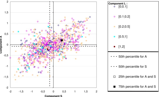
The object-based quality measure SAL defined by Wernli et al. (2008) was selected to verify the hourly AROME QPF. This method can evaluate three different aspects of the qual-ity of rainfall forecast fields over a specific domain: their structure (S), their location (L) and their amplitude (A). Their formulation is given in Appendix A. This method is suitable for the verification of QPF from convection-permitting weather prediction models on short time scales. It is also well-fitted to the object-based QPF perturbation method described in this paper.
The SAL method was applied to verify the hourly AROME QPF against the quantitative precipitation estimates (QPE) from radar data over the domainDshown in Fig. 1. The domain encloses the three watersheds but is a little larger than the area covered by them in order to better cope with the size of the mesoscale precipitation systems inducing heavy precipitation in that region. The 1 km2resolution radar QPE is based on the M´et´eo-France weather radar network and cal-ibrated by raingauges (Tabary, 2007, Tabary at al., 2007). The verification sample contained all the significant rainy events (24 days) that occurred over the domain from Octo-ber 2008 to OctoOcto-ber 2009. A rainy event was considered as significant if the daily rainfall exceeded 70 mm at least at one raingauge station of the domain. The SAL method was ap-plied to each hourly QPF in the 3 h to 24 h forecast range, as the two first hours of forecasting might have been damaged due to AROME spin-up. For each day of the sample, the four daily AROME operational simulations based on the analyses of 00:00, 06:00, 12:00 and 18:00 UTC, were available. Thus, the evaluation sample included more than 1100 hourly QPF
fields in total. The hourly QPF were not all independent, but this large number of fields permited us to assume that the comparison would not be biased.
The SAL method first requires individual precipitation ob-jects to be identified in both the observed and forecasted hourly rainfall fields. The precipitation objects are defined as continuous grid points exceeding a fixed threshold. Two different thresholds are used to enclose coherent objects in the threshold contour. A first threshold is fixed at a low value (2 mm h−1) to delineate the rainy areas (hereafter called “rainy objects”). Then a second higher value (9 mm h−1) enables the areas with convective rainfall (called hereafter “convective objects”) to be identified within the rainy ob-jects. This threshold has been found to be the most suit-able for capturing the convective signature of the precipitat-ing systems such as the convective line within the mesoscale convective systems observed over the region.
-2 -1,5 -1 -0,5 0 0,5 1 1,5 2
-2 -1,5 -1 -0,5 0 0,5 1 1,5 2
Component S
C
o
m
p
o
n
e
n
t
A
[0;0.1]
[0.1;0.2]
[0.2;0.5]
[0.5;1]
[1,2]
50th percentile for A
50th percentile for S
25th percentile for A and S
75th percentile for A and S Component L :
Fig. 2.SAL diagrams for the hourly precipitation forecast of AROME for the threshold 2 mm h−1. Every dot shows the value of the three components of SAL for a particular hour of the days of the sample. TheLcomponent is indicated by the colour of the dots (see scale on the top of the layout). Median values ofSandAare shown as dashed lines, the squares correspond to the 25th (white) and 75th (black) percentiles of the distributions ofSandA. (see Appendix A for more details).
-2 -1,5 -1 -0,5 0 0,5 1 1,5 2
-2 -1,5 -1 -0,5 0 0,5 1 1,5 2
Component S
C
o
m
p
o
n
e
n
t
A
[0;0.1]
[0.1;0.2]
[0.2;0.5]
[0.5;1]
[1,2]
50th percentile for A
50th percentile for S
25th percentile for A and S
75th percentile for A and S Component L :
Fig. 3.Same as Fig. 2, but for the threshold 9 mm h−1.
For the convective objects (Fig. 3), the S component is more frequently positive. Consequently, the simulated ob-jects are too-large and/or too-flat even when rainfall amounts are underestimated (i.e. in the bottom right quadrant). This occurs when the model predicts stratiform precipitation in a situation with intense localised showers.
The L component does not show systematic behaviour withSandAcomponents. Dots of any colour can be found in the four quadrants.
(a) Shift along X axes
0 1 2 3 4 5 6 7
(
%
)
[-5 ;5 ]
- 50 50
- 100 100
- 200 200
(Km)
(b) Shift along Y axes
0 1 2 3 4 5 6 7
(%
)
[-5 ;5 ]
- 50 50
- 100 100
- 200 200
(Km)
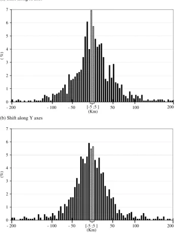
Fig. 4.Empirical pdf for location errors (km) alongX(a)andY (b) axes.
shift along the west-east (X) and north-south (Y) directions for each object. The values of the location errors are shown in Fig. 4a, b. The distance between the barycentre of sim-ulated and observed objects shows that in about 80 percent of the cases, the shift (in the either direction) does not ex-ceed 50 km. The amplitude error is computed as the ratio between mean surface precipitation within simulated and ob-served objects. This factor is calledf for rainy objects and fc for convective ones (Fig. 5a, b). The distribution offc
is well-centred around the value 1, whereas forf the ma-jor class is for a value between 0.8 and 0.9. Similar results were obtained whatever the range of the AROME forecast (not shown). This object-based approach shows that the de-terministic QPF on which the QPF perturbation ensemble will be built is not subject to systematic errors and provides a valuable possible scenario that is not too far from the ob-served one.
3.2 Perturbation generation
The method for generating an ensemble of rainfall forecasts is also based on an object-oriented approach taking advan-tage of the SAL evaluation. The perturbation method is based on the following principles:
(a) Rainy objects mean amplitude error
0 2 4 6 8 10 12 14 16 18
(Intensity factors values by intervals)
(%)
[0.9;1.1] 1.5
0.5 2
0 3 4
(b) Convective objects mean amplitude error
0 2 4 6 8 10 12 14 16 18
(Intensity factors values by intervals)
(%)
[0.9;1.1] 1.5
0.5 2
0 3 4
Fig. 5. Empirical pdf for amplitude error for rainy objects(a), co-efficientf and convective objects(b), coefficientfc. Values are
represented sorted by classes.
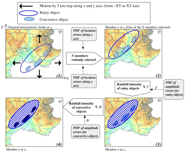
– The rainy objects are moved according to the pdf of the location errors of the AROME deterministic forecast. – The intensity of the rain inside the rainy objects is
mod-ified according to the pdf of the amplitude errors of the AROME deterministic forecast.
– The convective objects within each rainy object are set more or less peaked/flat according to the pdf of the am-plitude errors of the convective objects.
Motion by 5 km-step along x and y axes (from –XY to XY km)
N members radomly selected
Rainfall intensity of rainy objects x
y
Rainy object
Convective object
D
D D
D
X f
Rainfall intensity of convective
objects X fc PDF of location errors along x axis
PDF of location errors along y
axis PDF of amplitude
errors for rainy objects
PDF of amplitude errors for convective objects
f
fc
Original deterministic fields at t0 Membernatt0 (One of the Nmembers selected)
Membernatt0 Membernatt0
(1)
(1) (2)(2)
(3)
(3)
(4)
(4)
Fig. 6.Principle of the perturbation generation method at timet0.
by a factorf, randomly selected according to the pdf of the amplitude errors of the AROME deterministic forecast. Fi-nally, the rainfall intensity of each pixel of the convective objects within the rainy objects is multiplied by a factorfc,
randomly selected according to the pdf of the amplitude er-rors of the convective objects. The same displacement(x,y) and intensity factorsf andfcapply from forecasting range
t0to the final rangetf, to define a physically consistent
rain-fall scenario for each member. This method is called PERT-RAIN hereafter.
So PERT-RAIN has been designed to take advantage not only of the capabilities of the convection-permitting NWP models to produce rain fields of better quality that are more relevant to the hydrological scales involved in flash-flood forecasting, but also of the climatology of the AROME model errors, in terms of both amplitude and location. With this method, the spatial distribution of precipitation within the rainy object is not governed by statistical laws. It follows the physical dis-tribution given by the convection-permitting model that takes the synoptic meteorological situation, the orography and the meso-scale processes involved into account. Within Mediter-ranean heavy precipitation systems, the convective cells are not randomly distributed but generally organised along the
leading edge facing the marine low-level flow (Ducrocq et al., 2008). Our method retains this physical property. PERT-RAIN is applied to each hourly AROME QPF from 3 h (t0) to 24 h (tf) of the forecast. The reference
simula-tion PERT-RAIN considers 50 (N) members, which can be displaced up to±50 km (XY) along the x and y-axes, and have intensity factorsf andfc that can vary from 0.5 up to
1.5. Values ofN andXY are chosen considering the sensi-tivity analyses described in Sect. 5. The 50 rainfall scenarios are used to drive ISBA-TOPMODEL. The other parameters necessary to drive ISBA-TOPMODEL still come from the AROME deterministic operational forecast.
4 Ensemble streamflow forecast evaluation 4.1 Flash-flood cases
Hydrometeorological ensemble forecasts were performed for the two flash-flood events included in the AROME-PEARP evaluation period of Vi´e et al. (2010): 21–22 October 2008 and 1–2 November 2008.
Oct. case :
Nov. case :
(a)
(b)
Ardèche 0 500 1000 1500 2000 2500 3000 3500 4000 450021 o
ct -
12h
21 o
ct -
14h
21 o
ct -
16h
21 o
ct -
18h
21 o
ct -
20h
21 o
ct -
22h
22 o
ct -
00h
22 o
ct -
02h
22 o
ct -
04h
22 o
ct -
06h
22 o
ct -
08h
22 o
ct -
10h
22 o
ct -
12h
22 o
ct -
14h
22 o
ct -
16h
22 o
ct -
18h
22 o
ct -
20h
22 o
ct -
22h (m 3.s -1) Ardèche 0 500 1000 1500 2000 2500 3000 3500 4000 4500
01 n
ov -
12h
01 n
ov -
14h
01 n
ov -
16h
01 n
ov -
18h
01 n
ov -
20h
01 n
ov -
22h
02 n
ov -
00h
02 n
ov -
02h
02 n
ov -
04h
02 n
ov -
06h
02 n
ov -
08h
02 n
ov -
10h
02 n
ov -
12h
02 n
ov -
14h
02 n
ov -
16h
02 n
ov -
18h
02 n
ov -
20h
02 n
ov -
22h (m 3.s -1)
(c)
(d)
Cèze 0 200 400 600 800 1000 1200 1400 1600 1800 200021 o
ct -
12h
21 o
ct -
14h
21 o
ct -
16h
21 o
ct -
18h
21 o
ct -
20h
21 o
ct -
22h
22 o
ct -
00h
22 o
ct -
02h
22 o
ct -
04h
22 o
ct -
06h
22 o
ct -
08h
22 o
ct -
10h
22 o
ct -
12h
22 o
ct -
14h
22 o
ct -
16h
22 o
ct -
18h
22 o
ct -
20h
22 o
ct -
22h (m 3.s -1) Céze 0 200 400 600 800 1000 1200 1400 1600 1800 2000
01 n
ov -
12h
01 n
ov -
14h
01 n
ov -
16h
01 n
ov -
18h
01 n
ov -
20h
01 n
ov -
22h
02 n
ov -
00h
02 n
ov -
02h
02 n
ov -
04h
02 n
ov -
06h
02 n
ov -
08h
02 n
ov -
10h
02 n
ov -
12h
02 n
ov -
14h
02 n
ov -
16h
02 n
ov -
18h
02 n
ov -
20h
02 n
ov -
22h (m 3.s -1)
(e)
(f)
Gardons 0 500 1000 1500 2000 250021 o
ct -
12h
21 o
ct -
14h
21 o
ct -
16h
21 o
ct -
18h
21 o
ct -
20h
21 o
ct -
22h
22 o
ct -
00h
22 o
ct -
02h
22 o
ct -
04h
22 o
ct -
06h
22 o
ct -
08h
22 o
ct -
10h
22 o
ct -
12h
22 o
ct -
14h
22 o
ct -
16h
22 o
ct -
18h
22 o
ct -
20h
22 o
ct -
22h (m 3.s -1) 0 500 1000 1500 2000 2500
01 n
ov -
12h
01 n
ov -
14h
01 n
ov -
16h
01 n
ov -
18h
01 n
ov -
20h
01 n
ov -
22h
02 n
ov -
00h
02 n
ov -
02h
02 n
ov -
04h
02 n
ov -
06h
02 n
ov -
08h
02 n
ov -
10h
02 n
ov -
12h
02 n
ov -
14h
02 n
ov -
16h
02 n
ov -
18h
02 n
ov -
20h
02 n
ov -
22h
(m
3.s -1)
Gardons
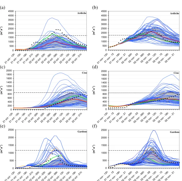
Fig. 7.Observed and forecast discharge time-series from 21 October 2008 at 12:00 UTC to 23 October 2008 at 00:00 UTC (left) and from 1 November 2008 at 12:00 UTC to 3 November 2008 at 00:00 UTC (right) over the three C´evennes-Vivarais watersheds: Ard`eche at Vallon Pont d’Arc(a, b); C`eze at Bagnols(c, d); Gardons at Boucoiran(e, f). Hourly observed discharge is plotted as black diamonds, forecast discharge with ISBA-TOPMODEL using the members of AROME-PEARP ensemble simulation as blue curves. The red curve is for the ensemble median. The shaded area represents the interquartile range. The green curve is the forecast discharge with ISBA-TOPMODEL using the AROME deterministic operational forecast. The orange curve is the simulated discharge with ISBA-TOPMODEL using the radar quantitative precipitation estimation. The dashed black line is the warning reference level used by the French operational flood forecasting centre.
frontal disturbance moving eastward was strengthened by the south to south-easterly convergent low-level flow that supplied moisture from the Mediterranean. The largest rainfall occurred over the foothills of the C´evennes on the evening of 21 October. Daily rainfall reached 470 mm at Le-Grand-Combe raingauge in the Gard department. This led to a significant rise of the water level of Gardons, C`eze and Ard`eche rivers. The AROME deterministic operational
forecast based on the 21 October at 12:00 UTC analysis produced high rainfall amounts over the C´evennes catch-ments. The rainy object location in the AROME forecast approximately matched the observed precipitation area but the convective part was underestimated in terms of both spatial extent and maximum rain intensity.
Table 1. Mean areal rainfall (mm) on 2 November 2008 from 00:00 UTC to 24:00 UTC over Gardons (at Boucoiran), C`eze (at Bagnols) and Ard`eche (at Vallon Pont d’Arc) from radar QPE and from AROME operational forecast based on the 2 November 2008 at 00:00 UTC analysis.
Catchment Boucoiran Bagnols/C`eze Vallon
(Gardons river) (C`eze river) (Ard`eche river)
AROME 113.7 94.8 255.6
RADAR 101.9 60.2 120.9
France from 31 October and evolved into a cut-off low over the Iberian peninsula by 2 November. A surface low pressure centre was located over southwestern France, which generated a rapid northward advection of moist, warm marine air. The C´evennes area was affected by heavy rain and river flooding. From 1 November 12:00 UTC to 2 November 12:00 UTC, around 400 mm were recorded locally over the Massif Central foothills. The AROME operational forecasts underestimated the maximum rainfall totals. 24h-accumulated precipitation reached no more than 200 mm. The rainy objects in the AROME forecasts were also located too far north compared to the observed ones. But the areal rainfall forecast (mean value on Gardons, C`eze and Ard`eche catchments) from the AROME deterministic operational forecast based on the 2 November 00:00 UTC analysis had values close to the observations or higher (see Table 1).
4.2 AROME-PEARP streamflow forecasts
A first set of streamflow ensemble forecasts was produced by the ISBA-TOPMODEL hydrological system driven by the eleven AROME-PEARP ensemble rainfall forecasts de-scribed in Sect. 2.2.2. This set constitutes our reference for evaluating the performance of the PERT-RAIN method in the following sections and for the sensitivity analyses. Fig-ure 7 shows the discharges simulated by ISBA-TOPMODEL using AROME-PEARP hourly rainfall ensemble members for the October and November cases. The discharge sim-ulation starts at 12:00 UTC (either on 21 October or on 1 November) and uses hourly QPF up to 24 h. The simula-tions are extended up to 36 h-range using zero rainfall in-tensity for the last 12 h to include the observed flood peak for the three catchments. The green and orange curves are for the discharges simulated by ISBA-TOPMODEL driven by the AROME deterministic forecast and the radar QPE, respectively. The shaded area in Fig. 7 represents the ensem-ble spread between quantilesq0.25andq0.75of the members. The dashed black line represents the warning level used in the national operational flood forecasting centre.
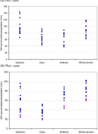
For both cases, the median of the members is generally closer to the observations or to the radar-driven simulation than the simulation driven by the AROME deterministic op-erational forecast. The radar-driven simulation helps to esti-mate the uncertainties associated with the hydrological mod-elling although some of the uncertainties come from the radar observations themselves. For all cases, both the median and the ensemble spread simulate a significant flood peak. This shows that this probabilistic approach introduces useful in-formation compared to the deterministic approach in both cases. Considering streamflow ensembles with respect to the warning level gives an idea of the risk of exceeding this level and so of being faced with a potentially dangerous situation. However, the quality of the results depends on the catchment and the case. Most of the time, the observed flood peak is included into the ensemble spread except for the Ard`eche watershed. For this watershed, the flood peak is underesti-mated by all the members for the October case and overesti-mated by most of the members for the Nov. case. Simulated discharges are of course strongly linked to the total precipi-tation falling over the watershed. For instance, the flow peak underestimation by all the members for the October case is well explained by rainfall totals smaller than the radar rain-fall estimate (Fig. 8).
4.3 Perturbed rainfall forecasts
The discharge time-series simulated by ISBA-TOPMODEL driven by the PERT-RAIN scenario are shown in Fig. 9. Many of the members lead to an underestimation of the dis-charge with no flood at all. Also some members strongly overestimate the peak flow. Nevertheless, the median and the interquartile range provide information about a flood oc-currence. The median is either closer to observations than the deterministic forecast or, at least, it informs on the risk of a flood which was already identified by the deterministic forecast. The stream flow ensemble is also informative as far as flow peak timing is concerned. Of course, encouraging as these results on two events may be, they need to be confirmed on more cases.
The PERT-RAIN interquartile range (shaded area in Fig. 9) is of the same order as our reference (AROME-PEARP). Overall, the PERT-RAIN median discharges are smaller than the AROME-PEARP ones, except for the November case over the Gardons watershed and for the October case for the Ard`eche watershed. The PERT-RAIN median flow peaks are generally closer to the observed ones or of the same accuracy as the AROME-PEARP median peaks, except for the Octo-ber case over the Gardons watershed. It is worth mentioning that even if the perturbation only concerns rainfall location and amplitude (not the rainfall time evolution), we obtained quite different precipitation time-evolution patterns over the watersheds with PERT-RAIN.
Table 2.Hourly discharges (m3.s−1) RPSS, RMSE andσof the ensembles AROME-PEARP and PERT-RAIN (10 members) at Boucoiran, Bagnols and Vallon Pont d’Arc. The values are written in bold when they are better than those of the competing experiment.
Catchment Boucoiran(Gardons river) Bagnols/C`eze (C`eze river) Vallon (Ard`eche river)
Ensemble AROME-PEARP PERT-RAIN AROME-PEARP PERT-RAIN AROME-PEARP PERT-RAIN
RPSS 0.30 0.19 0.06 −0.18 −0.06 −0.04
RMSE 185.8 173.3 158.1 104.6 504.7 462.1
σ 221.1 158.0 116.4 136.9 290.5 221.1
Table 3.Sensitivity experiments concerning the modification method.
Experiment name Modification applied Nvalues XY values
PERT-A Rainfall intensity only (f) 10 None
PERT-S Structure only (fc) 10 None
PERT-L Only location of 10 25 km/50 km
rainy objects modified
PERT-R[N] All modifications of the 10, 20, 30 50 km
PERT-RAIN (=PERT-R50) method 40, 50
The same number of members are considered for both the PERT-RAIN and AROME-PEARP methods to permit a fair comparison (Richardson, 2001). Only ten members were considered in PERT-RAIN so as to fit the AROME-PEARP ensemble size. In order to compare both streamflow ensem-bles in terms of mean error and spread, the Root Mean Square Error of the ensemble (RMSE) and the ensemble spread (σ) was computed for the hourly discharges at the three outlets. The reference was given by observed hourly discharges. An informative ensemble will lead to weak values of RMSE and to an order of magnitude of σ not higher than the RMSE one. Then, to evaluate the improvement with respect to the deterministic AROME forecast, the Ranked Probability Skill Score (RPSS) score was computed for the three catchments. RPSS gives an idea of the performance of an ensemble com-pared to a reference forecast (here the deterministic model). The values obtained are quite close for both methods. These scores confirm the visual inspection of the hydrograph: there is no method that systematically performs better than the other. For instance, PERT-RAIN obtains better scores than AROME-PEARP for the Ard`eche watershed whereas the op-posite is true for the C`eze river.
5 Sensitivity analyses
Some additional experiments were carried out to examine the sensitivity of the PERT-RAIN method to its degrees of free-dom. The characteristics of the sensitivity experiments are given in Table 3. The sensitivity experiments were eval-uated on the same October and November 2008 cases for
Quantitative Discharge Forecasts (QDF) but also on a larger sample of heavy precipitation events for QPF. As AROME forecasts have only been available since 2008, a compromise was made between building an independent evaluation sam-ple and a sufficient samsam-ple size. The QPF samsam-ple was thus composed of both the October and November 2008 events and five events with rainfall exceeding 70 mm day−1in 2009 and 2010. The four events in 2010 were outside the period used to establish the AROME error climatology on which the PERT-RAIN method is based. Scores were computed for 24-hour accumulated rainfall. The QDF was not evaluated on this period to save computer time and, also, discharge ob-servations have not yet been quality checked for this recent period.
Figure 10 shows the RPSS score computed on the 24-h rain-fall totals of the whole evaluation sample for all the sensitiv-ity experiments. Experiments PERT-RN with the number of membersNvarying from 50 to 10 (Table 3) allows an exam-ination of how much the PERT-RAIN method deteriorated with fewer members. As expected, decreasing the number of members deteriorates the RPSS score. The impact is larger when going from 10 to 20 members than when further enlarg-ing the ensemble size. Similar conclusions were drawn from QDF. The simulated hydrograms for experiments PERT-R10 to PERT-R50 for the Nov. case or October case (not shown) led to a median of the ensemble that fitted the observations better when the number of members was increased.
(a) Oct. case
0 20 40 60 80 100 120 140 160
Gardons Cèze Ardèche Whole domain
2
4
h
-a
c
c
u
m
u
la
te
d
p
re
c
ip
it
a
ti
o
n
(
m
m
)
(b) Nov. case
0 20 40 60 80 100 120
Gardons Cèze Ardèche Whole domain
2
4
h
-a
c
c
u
m
u
la
te
d
p
re
c
ip
it
a
ti
o
n
(
m
m
)
Fig. 8. 24h-accumulated rainfall (in mm) averaged over the three watersheds and over the whole domain from radar data (black crosses), the AROME deterministic operational forecast (pink cir-cle) and the members of the AROME-PEARP ensemble (blue points) between 21 October 2008 at 12:00 UTC and 22 Octo-ber 2008 at 12:00 UTC (a) and between 1 November 2008 at 12:00 UTC and 2 November 2008 at 12:00 UTC(b).
PERT-L experiment, only the location of the rainy objects was modified (step 1 of the perturbation method). In PERT-A only step 2, varying the amplitude of the rainy object through f, was kept. For the members of PERT-S, only the ampli-tude of the convective objects was modified (step 3 of the perturbation method) throughfc. These experiments were
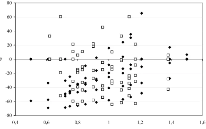
performed with 10 members only in order to reduce the com-putational cost. When only the location varied (PERT-L), keeping the sameXY=50 km maximum range as in the full PERT-RAIN ensemble, the RPSS value was slightly smaller than with the full method (PERT-R10). When the maximum range is reduced toXY=25 km, the skill was significantly reduced. The skill became negative which means that the en-semble forecast was less accurate than the reference. When the location of the forecasted objects was not modified in the perturbation method (for PERT-A and PERT-S experiments), the RPSS was further reduced (Fig. 10). Regarding the QDF, Fig. 11 presents the peak discharge error for each member according tof (for experiment PERT-A) orfc (for
experi-ment PERT-S) values. Although thefc pdf is almost
sym-metric, the QDF are underestimated for almost all values of fc. Even though the error is reduced with the larger values of
f, peak discharges remain underestimated most of the time. These results confirm the necessity of considering perturba-tions both in location and in amplitude. For the cases studied, the location perturbations had a larger impact than the ampli-tude perturbations. Allowing displacement of the rainy ob-jects up to 50 km for the perturbations is better for cases with larger errors in location of the AROME deterministic opera-tional forecast. These results are confirmed when the stream-flow ensemble obtained for experiments PERT-L, PERT-A, PERT-S and PERT-R is considered. The more satisfactory ensemble, on the basis of the two study cases of November 2008 and October 2008, was obtained for the PERT-R exper-iment, that is when location, amplitude and structure were perturbed.
6 Conclusions
Short-term precipitation ensemble forecasts for Mediter-ranean flash-floods can be produced from hourly forecasts issued by a convection-permitting meteorological determin-istic model. For this, a perturbation method has been de-veloped. The meteorological ensemble forecasts are fed into the ISBA-TOPMODEL model, which was specifically set up to simulate flash-floods to produce ensemble stream-flow forecasts. The perturbation method tries to take advan-tage of the high-resolution, process-based model trajectory of the new generation convection-permitting NWP forecasts. In addition, it also allows the uncertainty to be sampled in both location and magnitude of the precipitation forecast. This method makes use of the location and magnitude er-rors of the meteorological AROME model QPF in southeast-ern France.The SAL object-oriented verification method of Wernli et al. (2008) has been found to be well suited to sep-arately evaluating the errors of the rainfall forecasts in terms of location, amplitude and structure. No systematic biases of the AROME QPF have been found. More specifically the general drawback of underestimation of heavy precipitation by the coarser NWP models is not found for the convection-permitting AROME model. Errors in location do not exceed 50 km in 80 % of cases. Consequently, one can consider that AROME QPF are of good quality as far as heavy rain-fall is concerned. This justifies the approach developed for the PERT-RAIN perturbation method, directly based on the high-resolution model scenario and its simulated rainy ob-jects.
Oct. case :
Nov. case :
(a)
(b)
Ardèche 0 500 1000 1500 2000 2500 3000 3500 4000 450021 o
ct -
12h
21 o
ct -
15h
21 o
ct -
18h
21 o
ct -
21h
22 o
ct -
00h
22 o
ct -
03h
22 o
ct -
06h
22 o
ct -
09h
22 o
ct -
12h
22 o
ct -
15h
22 o
ct -
18h
22 o
ct -
21h (m 3.s -1) Ardèche 0 500 1000 1500 2000 2500 3000 3500 4000 4500
01 n
ov -
12h
01 n
ov -
15
01 n
ov -
18h
01 n
ov -
21
02 n
ov -
00h
02 n
ov -
03
02 n
ov -
06h
02 n
ov -
09
02 n
ov -
12h
02 n
ov -
15
02 n
ov -
18h
02 n
ov -
21 (m 3.s -1)
(c)
(d)
Cèze 0 200 400 600 800 1000 1200 1400 1600 1800 200021 o
ct -
12h
21 o
ct -
15h
21 o
ct -
18h
21 o
ct -
21h
22 o
ct -
00h
22 o
ct -
03h
22 o
ct -
06h
22 o
ct -
09h
22 o
ct -
12h
22 o
ct -
15h
22 o
ct -
18h
22 o
ct -
21h (m 3.s -1) Cèze 0 200 400 600 800 1000 1200 1400 1600 1800 2000
01 n
ov -
12h
01 n
ov -
15
01 n
ov -
18h
01 n
ov -
21
02 n
ov -
00h
02 n
ov -
03
02 n
ov -
06h
02 n
ov -
09
02 n
ov -
12h
02 n
ov -
15
02 n
ov -
18h
02 n
ov -
21 (m 3.s -1)
(e)
(f)
Gardons 0 500 1000 1500 2000 250021 o
ct -
12h
21 o
ct -
15h
21 o
ct -
18h
21 o
ct -
21h
22 o
ct -
00h
22 o
ct -
03h
22 o
ct -
06h
22 o
ct -
09h
22 o
ct -
12h
22 o
ct -
15h
22 o
ct -
18h
22 o
ct -
21h (m 3.s -1) Gardons 0 500 1000 1500 2000 2500
01 n
ov -
12h
01 n
ov -
15
01 n
ov -
18h
01 n
ov -
21
02 n
ov -
00h
02 n
ov -
03
02 n
ov -
06h
02 n
ov -
09
02 n
ov -
12h
02 n
ov -
15
02 n
ov -
18h
02 n
ov -
21
(m
3.s -1)
Fig. 9.Same as Fig. 7, but ISBA-TOPMODEL is driven by the members of the PERT-RAIN ensemble.
state-of-the-art research convection-permitting NWP ensem-ble (AROME-PEARP). The sensitivity analyses show that an ensemble size larger than 20 members provides better skill regarding the deterministic forecast than ensembles with fewer members. The perturbations in location have the strongest impact on the skill of the ensemble. However, the best ensemble, in terms of both precipitation forecast and streamflow simulation, was obtained when the three kinds of perturbation were combined (location, amplitude and struc-ture). Further verification on a larger size sample of flash-flood cases is still needed to confirm these promising re-sults. The observing periods of the HYMEX field experiment (http://www.hymex.org) will also provide a test-bed for eval-uating the method in a real-time framework.
The PERT-RAIN method is based on the pdf of AROME QPF errors. Completing our climatology of those errors will be a way to improve the skill and reliability of the PERT-RAIN ensemble. For instance, it could be useful to determine location error in terms of distance rather than using x and y coordinates errors and also to determine different PDFs for each forecast range.
convection--0,4 -0,3 -0,2 -0,1 0 0,1 0,2 0,3 0,4
PER T-A
PER T-S
PER T-L
XY =25
PER T-L
XY =50
PER T-R
10
PER T-R
20
PER T-R
30
PER T-R
40
PER T-R
50
R
P
S
S
Fig. 10. 24h-accumulated rainfall (mm day−1) RPSS for the en-sembles obtained with experiments PERT-A withN=10, PERT-S withN=10, PERT-L withN=10 and XY = 25 km, PERT-L with
N=10 and XY = 50 km, PERT-RN with XY = 50 km and varying the number of members (N).
-80 -60 -40 -20 0 20 40 60 80
0,4 0,6 0,8 1 1,2 1,4 1,6
%
Fig. 11. Flood peak errors in percentages in function off (filled diamonds) andfc(blank squares) values.
permitting NWP ensembles in order to enlarge the size of the ensemble. Considering their cost, the size of such convection-permitting NWP ensembles should still be lim-ited (around 10–20 members) in the foreseeable future. The PERT-RAIN method addresses the first source of uncer-tainty in flash-flood hydrological forecasting, that is QPF un-certainties. Other hydrological uncertainties, such as those associated with the initial soil moisture content or with the hydrological modelling system itself, will also be examined in the future in order to sample the total uncertainty associ-ated with Mediterranean flash-flood forecasting.
Appendix A
Definition of the three components of SAL (Wernli et al., 2008)
SAL is an object-based quality measure, which evaluates three components concerning the structure of the precipita-tion field (S), its amplitude (A) and its location (L). This measure is valid for a given geographical domainD. It is based on the differences between a simulated precipitation fieldRmodand the observed fieldRobs.
The A component is the normalised difference of the domain-averaged precipitation values:
A=2.Rmod−Robs Rmod+Robs
(A1) It is a relative measure of the bias of the model over the do-mainD. Values of the A component are between−2 and +2 and a perfect forecast corresponds toA=0.
Evaluation ofSandLrequires the identification of coher-ent precipitation objects in both forecast and observation.
The location componentLis the sum of two contributions denotedL1andL2. L1is the normalised distance between the barycentre of the simulated field (x(Rmod)) and that of the observed field (x(Robs)) over the whole domainD.
L1=|x(Rmod)−x(Robs)|
d (A2)
withdthe maximum distance possible between two points of the domainD. L2 takes into account the mean distance be-tween the barycentre of the whole precipitation field (x) and the barycentre of each individual object (xn) This function is
denotedr: r=
PM
n=1Rn|x−xn|
PM
n=1Rn
(A3) whereMis the total number of individual objects in the field, andRnis the integrated amount of precipitation for the object
n.L2is then given by: L2=2|rmod−robs|
d (A4)
L (=L1+L2)allows the global shift of the simulated field to be evaluated with respect to the observation. It also gives information about the spatial precipitation distribution. Val-ues of the L-component are between 0 and +2 and a perfect forecast corresponds toL=0.
The structure component S is based on the “scaled vol-ume” of each precipitation objectVn:
Vn=
Rn
Rmax
n
(A5) whereRnmaxis the maximum rainfall value within the object
For the whole field, one can compute the weighted mean precipitation volume of all objects denotedV:
V=
PM
n=1Rn.Vn
PM
n=1Rn
(A6) Sis then the normalised difference between observed and simulatedV:
S=2.Vmod−Vobs Vmod+Vobs
(A7) Values of theS component are between −2 and +2 and a perfect forecast corresponds toS=0. Positive values ofS
correspond to simulated objects that are too-large compared to the observed ones or to a widespread simulated precipita-tion field when the observed field presents small convective events, i.e. the simulated objects are too flat. Conversely, negative values ofS correspond to too-small or too-peaked simulated objects.
Appendix B Statistical tools
The skill of ensemble predictions (rainfall and streamflows) is evaluated in the study through the root mean square er-ror (RMSE), the spread (σ) and the ranked probability skill score. The RMSE is defined as:
RMSE= v u u
t1
N
N
X
i=1
(mi−oi)2 (B1)
whereN is the total number of time steps,oi the reference
value at time stepiandmi the mean of the forecast members.
The spread is computed as:
σ= 1 N
N
X
i=1
v u u t 1 n
n
X
k=1
(xk,i−mi)2 (B2)
wherenis the number of forecast members andxk,ithe value
of memberkat time stepi.
The Ranked Probability Score (RPS) derives from the Brier Score (BS) (Brier, 1950; Wilks, 1995). It considers the exceedance of K-1 thresholds. The forecasts are divided into K classes.
RPS= 1 K−1
K
X
k=1
[Yk−Ok]2 (B3)
whereYk andOkare the cumulated k threshold distributions
for forecasts and observations respectively. RPS varies be-tween 0 and+∞;0 is for a perfect forecast. Then the Ranked Probability Skill Score (RPSS) situates the forecasted ensem-ble with respect to a reference forecast:
RPSS=1− RPS RPSref
(B4)
RPSS varies between−∞and 1; 1 corresponds to a perfect forecast.
Acknowledgements. This work was carried out in the framework of the MEDUP project (Grant ANR-07-VULN-06-001), funded by the Vuln´erabilit´e Milieux et Climat (VMC) programme of the National Research Agency (ANR).
Edited by: G. Molinie
Reviewed by: M.-H. Ramos and two other anonymous referees
The publication of this article is financed by CNRS-INSU.
References
Anquetin, S., Yates, E., Ducrocq, V., Samouillan, S., Chancibault, K., Davolio, S., Accadia, C., Casaioli, M., Mariani, S., Ficca, G., Gozzini, B., Pasi, F., Pasqui, M., Garcia, A., Martorell, M., Romero, R., and Chessa, P.: The 8 and 9 September 2002 flash flood event in France: a model intercomparison, Nat. Hazards Earth Syst. Sci., 5, 741–754, doi:10.5194/nhess-5-741-2005, 2005.
Bartholmes and Todini: Coupling meteorological and hydrological models for flood forecasting, Hydrol. Earth Syst. Sci., 9, 333– 346, doi:10.5194/hess-9-333-2005, 2005.
Beaulant, A.-L., Joly, B., Nuissier, O., Somot, S., Ducrocq, V., Joly, A., Sevault, F., D´equ´e, M., and Ricard, D.: Statistico-dynamical downscaling for Mediterranean heavy precipitation, Q. J. Roy. Meteorol. Soc., 137 (656), 736–748, doi:10.1002/qj.796, 2011.
Bernard, P.: Aladin/AROME dynamical core, status and
possible extension to IFS, in: ECMWF Seminar
Pro-ceedings, September 2004, http://www.ecmwf.int/publications/ libraryinNOV.2004, 2004.
Beven, K. and Kirkby, M. J.: A physically based, variable contribut-ing area model of basin hydrology, Hydrol. Sci. Bull., 24, 43–69, 1979.
Beven, K. and Freer, J.: Equifinality, data assimilation, and uncer-tainty estimation in mechanistic modelling of complex environ-mental systems using the GLUE methodology, J. Hydrol., 249, 11–29, 2001.
Bouilloud, L., Chancibault, K., Vincendon, B., Ducrocq, V., Habets, F., Saulnier, G. M., Anquetin, S., Martin, E., and Noilhan, J.: An advanced coupling between the ISBA land surface model and the TOPMODEL hydrological model to simulate Mediterranean flash-floods, J. Hydrometeor., 11(2), 315–333, 2010.
Brier, G. W.: Verification of forecasts expressed in terms of proba-bility, Mon. Weather. Rev., 78, 1–3, 1950.
Bowler, N., Pierce, C., and Seed, A.: STEPS: A probabilistic precipitation forecasting scheme which merges an extrapolation nowcast with downscaled NWP, Q. J. Roy. Meteorol. Soc., 132, 99, 132, 2127–2155, 2006.
pressure terrain-following coordinate in the framework of ARPEGE/ALADIN NWP system, Mon. Weather. Rev., 123, 515–535, 1995.
Caniaux, G., Redelsperger, J. L., and Lafore J. P.: A numerical study of the stratiform region of e fast-moving squall line. Part I. Gen-eral description and water and heat budgets, J. Atmos. Sci., 51, 2046–2074, 1994.
Chancibault, K., Anquetin, S., Ducrocq, V., and Saulnier, G.-M.: Hydrological evaluation of high resolution precipitation forecasts of the Gard flash-flood event (8–9 September 2002), Q. J. Roy. Meteor. Soc., 132, 1091–1117, 2006.
Cloke, H.-L. and Pappenberger, F.: Ensemble flood forecasting: a review, J. Hydrol., 375(3–4), 613–626, 2009.
Courtier, P., Freydier, C., Geleyn, J.-F., Rabier, F., and Rochas, M.: The ARPEGE project at M´et´eo-France, in: Workshop on numer-ical methods in atmospheric models, Reading, UK, ECMWF, 2, 193–231, 1991.
Davolio, S., Miglietta, M. M., Diomede, T., Marsigli, C., Morgillo, A., and Moscatello, A.: A meteo-hydrological prediction system based on a multi-model approach for precipitation forecasting, Nat. Hazards Earth Syst. Sci., 8, 143–159, doi:10.5194/nhess-8-143-2008, 2008.
Deidda, R.: Rainfall downscaling in a space multifractal frame-work, Water Res. Res., 36, 1779–1794, 2000.
Diomede, T., Marsigli, C., Nerozzi, F., Paccagnella, T., and Mon-tani, A.: Quantifying the discharge forecast uncertainty by differ-ent approaches to probabilistic quantitive precipitation forecast, Adv. Geosci., 7, 189–191, 2006,
http://www.adv-geosci.net/7/189/2006/.
Diomede, T., Marsigli, C., Nerozzi, F., Papetti, P., and Paccagnella, T.: Coupling high-resolution precipitation forecasts and dis-charge predictions to evaluate the impact of spatial uncertainty in numerical weather prediction model outputs, Meteor. Atmos. Phys., 102, 1–2, 37–62, 2008.
Ducrocq V., Nuissier, O., Ricard, D., Lebeaupin, C., and Thou-venin, T.: A numerical study of three catastrophic precipitat-ing events over southern France. II: Mesoscale triggerprecipitat-ing and stationarity factors, Quart. J. Roy. Meteor. Soc., 134, 131–145, doi:10.1002/qj.199, 2008.
Ferraris, L., Rudari, R., and Siccardi, F.: The uncertainty in the prediction of flash-floods in the northern Mediterranean environ-ment, J. Hydrometeor., 3, 714–726, 2002.
Habets, F., Boone, A., Champeaux, J. L., Etchevers, P., Franchis-teguy, L., Leblois, E., Ledoux, E., Le Moigne, P., Martin, E., Morel, S., Noilhan, J., Quintana-Segui, P., Rousset-Regimbeau, F., and Viennot, P.: The SAFRAN-ISBA-MODCOU hydrome-teorological model applied over France, J. Geophys. Res., 113, D06113, doi:10.1029/2007JD008548, 2008.
Hamill, T. M., Hagedorn, R., and Whitaker, J. S.: Probabilistic fore-cast calibration using ECMWF and GFS ensemble forefore-casts. Part II: Precipitation, Mon. Weather Rev., 136, 7, 2620–2632, 2007. Jasper, K., Gurtz, J., and Lang, H.: Advanced flood forecasting in
Alpine watersheds by coupling meteorological observations and forecasts with a distributed hydrological model, J. Hydrol., 267, 40–52, 2002.
Komma, J., Reszler, C., Bl¨oschl, G., and Haiden, T.: Ensem-ble prediction of floods – catchment non-linearity and fore-cast probabilities, Nat. Hazards Earth Syst. Sci., 7, 431–444, doi:10.5194/nhess-7-431-2007, 2007.
Krzysztofowicz, R.: Bayesian system for probabilistic river stage forecasting, J. Hydrol., 268, 16–40, 2002.
Lafore, J. P., Stein, J., Asencio, N., Bougeault, P., Ducrocq, V., Duron, J., Fischer, C., Hreil, P., Mascart, P., Masson, V., Pinty, J. P., Redelsperger, J. L., Richard, E., and Vil`a-Guerau de Arel-lano, J.: The Meso-NH Atmospheric Simulation System. Part I: adiabatic formulation and control simulations, Ann. Geophys., 16, 90–109, doi:10.1007/s00585-997-0090-6, 1998.
Le Lay, M. and Saulnier, G. M.: Exploring the signature of spatial variabilities in flash flood events: Case of the 8–9 September 2002 C´evennes-vivarais catastrophic event, Geophys. Res. Lett., 34, L13401, doi:10.1029/2007GL029746, 2007.
Llasat, M. C.: Chapter 18: Storms and floods, in: The Physical Geography of the Mediterranean basin, edited by: J. Woodward, Published by Oxford University Press, 504–531, 2009.
Ludwig, R., Taschner, S., and Mauser, W.: Modelling floods in the Ammer catchment: limitations and challenges with a coupled meteo-hydrological model approach, Hydrol. Earth Syst. Sci., 7, 833–847, doi:10.5194/hess-7-833-2003, 2003.
Marsigli, C., Boccanera, F., Montani, A., and Paccagnella, T.: The COSMO-LEPS mesoscale ensemble system: validation of the methodology and verification, Nonlin. Processes Geophys., 12, 527–536, doi:10.5194/npg-12-527-2005, 2005.
Melone, F., Barbetta, S., Diomede, T., Perucacci, S., Rossi, M., Tessarollo, A., and Verdecchia, M.: Review and selec-tion of hydrological models – Integraselec-tion of hydrological mod-els and meteorological inputs, Resulting from Work Package 1, Action 13, RISK AWARE – INTERREG III B – CAD-SES, 34 pp., http://www.smr.arpa.emr.it/riskaware/get.php?file= ReportWP1.13.pdf, 2005.
Molteni, F., Buizza, R., Palmer, T. N., and Petroliagis, T.: The ECMWF Ensemble Prediction System: Methodology and Val-idation, Q. J. Roy. Meteor. Soc., 122, 73–119, 1996.
Montanari, A.: Large sample behaviours of the generalized likeli-hood uncertainty estimation (GLUE) in assessing the uncertainty of rainfall-runoff simulations, Water Resour. Res., 41, W08406, doi:10.1029/2004WR003826, 2005.
Nicolau, J.: Short-range ensemble forecasting. WMO/CSB Tech-nical Conference meeting, Cairns (Australia), December 2002 (Proceedings), 2002.
Noilhan, J. and Planton, S.: A simple parametrization of land sur-face processes for meteorological models, Mon. Weather. Rev., 117, 536–549, 1989.
Pellarin, T., Delrieu, G., Saulnier, G. M., Andrieu, H., Vignal, B., and Creutin, J. D.: Hydrological visibility of weather radars oper-ating in mountainous regions: case study for the Ard`eche catch-ment, France, J. Hydrometeor., 3, 5, 539–555, 2002.
Randrianasolo, A., Ramos, M. H., Thirel, G., Andrassian, V., and Martin, E.: Comparing the scores of hydrological ensemble fore-casts issued by two different hydrological models, Atmos. Sci. Lett., 11, 2, 100–107, 2010.
Regimbeau, F. R., Habets, F., Martin, E., and Noilhan, J.: Ensemble streamflow forecasts over France, ECMWF Newsletter, 111, 21– 27, 2007.
Richardson, D.: Measures of skill and value of ensemble prediction systems, their interrelationship and the effect of ensemble size, Quart. J. Roy. Meteor. Soc., 127, 2473–2489, 2001.
forecasts for advance warning of the Carlisle flood, north-west England, Meteorol. App., 16(1), 23–44, doi:10.1002/met.94, 2009.
Rotach, M. W., Ambrosetti, P., Ament, F., Appenzeller, C., Arpa-gaus, M., Bauer, H.-S., Behrendt, A., Bouttier, F., Buzzi, A., Corazza, M., Davolio, S., Denhard, M., Dorninger, M., Fontan-naz, L., Frick, J., Fundel, F., Germann, U., Gorgas, T., Hegg, C., Hering, A., Keil, C.,. Liniger, M., Marsigli, C., McTaggart-Cowan, R., Montaini, A., Mylne, K., Ranzi, R., Richard, E., Rossa, A., Santos-Muoz, D., Schr, C., Seity, Y., Staudinger, M., Stoll, M., Volkert, H., Walser, A., Wang, Y., Werhahn, J., Wulfmeyer, V., and Zappa, M.: MAP D-PHASE: Real-time Demonstration of Weather Forecast Quality in the Alpine Re-gion, B. Am. Meteor. Soc., doi:10.1175/2009BAMS2776.1, 90, 1321–1336, 2009.
Schaake, J. C., Hamill, T. M., Buizza, R., and Clark, M.: HEPEX: the Hydrometeorological Ensemble Prediction EXperiment, J. Hydrometeor., 88, 1541–1547, 2007.
Seity, Y., Brousseau, P., Malardel, S., Hello, G., Bernard, P., Bout-tier, F., Lac C., and Masson, V.: The AROME-France convective scale operational model, Mon. Weather. Rev., 139(3), 976–991, 2010.
Siccardi, F., Boni, G., Ferraris, L., and Rudari, R.: A Hydromete-orological approach for probabilistic flood forecast, J. Geophys. Res., 110, D05101, doi:10.1029/2004JD005314, 2005.
Tabary, P.: The new French radar rainfall product. Part I : method-ology, Weather Forecast., 22, 3, 393–408, 2007.
Tabary, P., Desplats, J., Do Khac, K., Eideliman, F., Gueguen, C., and Heinrich, J.-C.: The new French radar rainfall product. Part II : Validation, Wea. Forecast., 22, 3, 409–427, 2007.
Theis, S. E., Hense, A., and Damrath, U.: Probabilistic precipita-tion forecasts from a deterministic model: a pragmatic approach, Meteorol. Appl., 12, 257–268, 2005.
Thielen, J., Schaake, J., Hartman, R., and Buizza, R.: Aims, chal-lenges and progress of the Hydrological Ensemble Prediction EXperiment (HEPEX) following the third HEPEX workshop held in Stresa 27 to 29 June 2007, Atmos. Sci. Lett., 9, 29–35, 2008.
Thielen, J., Bartholmes, J., Ramos, M.-H., and de Roo, A.: The Eu-ropean Flood Alert System – Part 1: Concept and development, Hydrol. Earth Syst. Sci., 13, 125–140, doi:10.5194/hess-13-125-2009, 2009.
Thirel, G., Rousset-Regimbeau, F., Martin, E., and Habets, F.: On the impact of short-range meteorological forecasts for ensem-ble stream flow predictions, J. Hydrometeorol., 9, 6, 1301–1317, 2008.
Thirel, G., Regimbeau, F., Martin, E., Noilhan, J., and Habets, F.: Short-and medium-range hydrological ensemble forecasts over France, Atmos. Sci. Lett., 11, 2, 72–77, 2010.
Vi´e, B., Nuissier, O., and Ducrocq, V.: Cloud-resolving ensemble simulations of heavy precipitating events: uncertainty on initial conditions and lateral boundary conditions, Mon. Weather. Rev., 139, 403–423, doi:10.1175/2010MWR3487.1, 2010.
Vincendon, B., Ducrocq, V., Dierer, S., Kotroni, V., Le Lay, M., Milelli, M., Quesney, A., Saulnier, G.-M., Rabuffetti, D., Bouil-loud, L., Chancibault, K., Anquetin, S., Lagouvardos, K., and Steiner, P.: Flash flood forecasting within the PREVIEW project: value of high-resolution hydrometeorological coupled forecast, Meteor. Atmos. Phys., 103, 115–125, 2009.
Vincendon, B., Ducrocq, V., Saulnier, G. M., Bouilloud, L., Chancibault, K., Habets, F., and Noilhan, J.: Benefit of coupling the ISBA land surface model with a TOPMODEL hydrological model dedicated to Mediterranean flash floods, J. Hydrol., 394, 256–266, doi:10.1016/j.jhydrol.2010.04.012, 2010.
Wernli, H., Paulat, M., Hagen, M., and Frei, C.: SAL-A novel qual-ity measure for the verification of quantitative precipitation fore-casts, 2008, Mon. Weather. Rev., 136, 4470–4487, 2008. Wilby, R. L. and Wigley, T. M. L.: Downscaling general circulation
model output: a review of methods and limitations, Prog. Phys. Geogr., 21, 530–548, 1997.
Wilks, D. S.: Statistical methods in the Atmospheric sciences: An introduction, Academic Press, 467 pp., 1995.
Xu, C.: From GCMs to river flow: a review of downscaling methods and hydrologic modelling approaches, Prog. Phys. Geogr., 23(2), 229–249, 1999.
Xuan, Y., Cluckie, I. D., and Wang, Y.: Uncertainty analysis of hydrological ensemble forecasts in a distributed model utilising short-range rainfall prediction, Hydrol. Earth Syst. Sci., 13, 293– 303, doi:10.5194/hess-13-293-2009, 2009.
Zappa, M., Beven, K., Bruen, M., Cofio, A., Kok, K., Martin, E., Nurmi, P, Orfila, B., Roulin, E., Schrater, K, Seed, A, Szturc, J., Vehvilinen, B., Germann, U., and Rossa, A.: Propagation of uncertainty from observing systems and NWP into hydrological models: COST-731 Working Group 2, Atmos. Sci. Lett., 11(2), 83–91, 2010.