www.nonlin-processes-geophys.net/21/393/2014/ doi:10.5194/npg-21-393-2014
© Author(s) 2014. CC Attribution 3.0 License.
Nonlinear Processes
in Geophysics
Provision of boundary conditions for a convection-permitting
ensemble: comparison of two different approaches
C. Marsigli, A. Montani, and T. Paccagnella
ARPA-SIMC, HydroMeteoClimate Service of ARPA Emilia-Romagna, Bologna, Italy
Correspondence to:C. Marsigli ([email protected])
Received: 26 July 2013 – Revised: 20 December 2013 – Accepted: 9 January 2014 – Published: 12 March 2014
Abstract. The current resolution of the operational global models favours the possibility of driving convection-permitting limited-area model (LAM) simulations directly, sparing the necessity for an intermediate step with a coarser-resolution LAM. Though the coarser-resolution of global ensemble systems is generally lower than that of deterministic ones, it is also possible to consider this opportunity in the field of ensemble forecasting. The aim of this paper is to investigate the effect of this choice for driving a convection-permitting ensemble based on the COSMO model, for a specific ap-plication, namely the forecast of intense autumn precipita-tion events over Italy. The impact of the direct nesting in the ECMWF global ensemble is compared to a two-step nesting, which makes use of a LAM ensemble system with parametrised convection. Results show that the variability in-troduced in the geopotential field by the direct nesting is usu-ally contained within the uncertainty described by the stan-dard ensemble, and differences between pairs of members following different nesting approaches are generally smaller than the ensemble error, computed with respect to analy-sis. The relation between spread and error is even improved by the direct nesting approach. In terms of precipitation, it is found that the forecasts issued by members with differ-ent nesting approaches generally have differences at spatial scales between 16 and 180 km, depending on the case, hence not negligible. Nevertheless, the skill of the LAM ensemble precipitation forecasts, evaluated by means of an objective verification, is comparable. Therefore, the overall quality of the 2.8 km ensemble for the specific application is not deteri-orated by the provision of lower resolution lateral boundary conditions directly from the global ensemble.
1 Introduction
The current resolution of operational global circulation models (GCM) paves the way towards driving convection-permitting limited-area model (LAM) integrations directly, with lateral boundary conditions (LBCs) provided by a global model. Presently, high-resolution LAM runs are gen-erally nested in coarser-resolution integrations of the same model. The intermediate step with a coarser-resolution run is usually performed to ensure a ratio of spatial resolutions between nested models in the range of 2:1–5:1. The aim is to reduce the loss of information due to nesting which would affect the nested model in the case of a larger resolution gap (see for example Warner et al., 1997 and Denis et al., 2001). With the resolution increase of the GCMs, the intermediate step with a coarser-resolution LAM could be avoided, with some potential benefits. First of all, removing one step in the nesting procedure would decrease the time needed to perform the whole cascade up to the convection-permitting integra-tion, with a consequent reduction of the computational costs. This would be most beneficial in an operational environment, requiring timely delivery of products. Secondly, one short-coming of the intermediate LAM run is that nowadays this usually runs in the so-called “grey zone”, where convection is partly resolved and partly sub-grid. This is recognised to be a delicate issue for many models (see e.g. Gerard et al., 2009). On the other hand, the coarser spatial and temporal resolution of the LBCs provided by a global model could in-troduce errors in the forecast, especially if the LAM domain is small, as is often the case for convection-permitting mod-els. Some studies have addressed this issue.
is true if boundaries are set far from the region of inter-est, which is usually not true for convection-permitting sim-ulations. Temporal resolution is also an issue, since LBCs are often produced at much lower frequency than the time step used in the LAM. If information changes rapidly at the boundary, then the LBCs might not reflect the actual changes in the state of the atmosphere (Termonia et al., 2009). Termo-nia (2003) found that the use of a coupling update interval of 3 h has a detrimental effect on the forecast quality of a very intense storm, affecting significantly the depth of the low-pressure system. Davies (2014) showed that, with an 11 km resolution model, 3-hourly LBCs already lead to a loss of information with respect to hourly LBCs at a 12 h forecast range. Amengual et al. (2007) found that for regional climate model (RCM) runs the update frequency of LBCs has a larger impact on the downscaling results than their spatial resolu-tion. Nevertheless, the ratio between the two factors is de-pendent on the actual resolutions involved and on the forecast range. As for the relation between the two effects and their impact on LAM ensembles, Nutter et al. (2004) showed that the impact of coarsely resolved LBCs or temporal interpola-tion of LBCs on error growth is quite similar. Both effects act to remove small-scale features from the external fields passing through the lateral boundary, thereby constraining ensemble dispersion. The impact of coarsely resolved LBCs has been identified as stronger than the one of temporal inter-polation when the LBC update frequency is reasonably high. In this work, the issue of LBC resolution is considered in the framework of ensemble forecasting. The aim of this pa-per is to investigate the effect of the provision of LBCs to a LAM ensemble run at a convection-permitting resolution by a global ensemble, compared with providing LBCs from an intermediate LAM ensemble run at coarser resolution. The analysis is confined to a specific meteorological situation, namely autumn precipitation cases over the Mediterranean.
Aiming at the development of an ensemble system at the convection-permitting scale over Italy, ARPA-SIMC has im-plemented an experimental ensemble based on the COSMO model (Steppeler et al., 2003) during SOP (Special Obser-vation Period) 1.1 of the Hymex Project (HYMEX, 2010– 2020). The ensemble, named COSMO-H2-EPS (COSMO Hymex 2.8 km Ensemble Prediction System, Marsigli et al., 2013), consists of 10 runs of the COSMO model at 2.8 km horizontal resolution, with 50 levels in the vertical, and re-ceives perturbed ICs and LBCs from the first 10 members of COSMO-LEPS (COSMO Limited-area Ensemble Predic-tion System, Montani et al., 2011). COSMO-LEPS, running at 7 km horizontal resolution with parametrised convection, in turn receives initial and boundary conditions from the global ensemble of ECMWF, referred to as ENS. ENS is cur-rently running with an approximate horizontal resolution of 32 km, which is planned to increase to about 20 km in 2015. This may enable direct use of LBCs from ENS members to drive ensemble systems for the convection-permitting scale (2–3 km).
In this work, it is studied how the performance of the COSMO-H2-EPS ensemble varies if the 2.8 km runs receive ICs and BCs from the ENS members directly, skipping the intermediate step with COSMO-LEPS at 7 km. The aim is to evaluate the effect of removing this step, heading for the future operational set-up of the ensemble, which will benefit from the resolution increase of ENS, up to 20 km. Though in the present configuration the resolution gap between driv-ing model (32 km, retrieved on a grid of 0.25◦
mesh size) and driven model (2.8 km) is quite high, it is believed that an assessment of the difference between the two nesting proce-dures on the specific ensemble application can provide sci-entific guidance useful for defining the operational set-up. It is also worth mentioning that, in its operational configura-tion, the 2.8 km ensemble will not use as ICs the downscaled ENS analyses, since high-resolution perturbed initial condi-tions will be provided by a LETKF scheme developed in the COSMO consortium (KENDA system, Reich et al., 2011), which is currently under testing.
The paper is organised as follows: in the next section, the configuration of the ensembles is described. Then, in Sect. 3 results are commented on, divided into an analysis of fields of geopotential at 500 hPa and precipitation. Finally, conclu-sions are drawn in Sect. 4.
2 Configuration of the ensemble systems
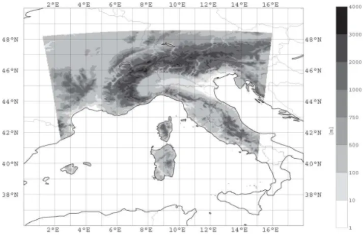
COSMO-H2-EPS is an ensemble system specifically de-signed for the Hymex Project, which was run regularly dur-ing SOP 1.1, takdur-ing place from 5 September to 6 Novem-ber 2012. The ensemble consists of 10 runs of the COSMO model at 2.8 km horizontal resolution, with 50 levels in the vertical, over a domain including most of the target areas of the project. In particular, it covers a large part of Italy, Switzerland and the French Mediterranean coast (Fig. 1). The model domain contains 399×412 grid points. The ensemble was run once per day, starting at 12:00 UTC, for a forecast range of 36 h.
be highlighted that this same model perturbation technique is adopted in COSMO-LEPS, with some differences in the pa-rameters which are perturbed. These pertubations affect the model run starting from the first time step, but do not af-fect the analysis, therefore ICs are not changed due to model perturbation. For a comprehensive description of the two systems the reader is referred to Marsigli et al. (2013) for H2-EPS and to Montani et al. (2011) for COSMO-LEPS.
A second experimental ensemble, named EXP-H2-EPS, has been implemented for the present study. It has been run for 21 cases of the SOP 1.1 period, selected as events of mod-erate to intense (observed) precipitation. A description of the meteorological situation during the SOP and of a few severe events can be found in Ducrocq et al. (2013) and Ferretti et al. (2013) (the latter focussing on Italy).
The ensemble configuration of EXP-H2-EPS is identi-cal to that of COSMO-H2-EPS in terms of resolution, do-main, model set-up, and parameter perturbation. The only difference is in the way ICs and BCs are provided: for EXP-H2-EPS they are derived directly from 10 members of ENS, the same members that have been selected to drive the first 10 COSMO-LEPS operational runs. Therefore, pairs of members of EXP-H2-EPS and COSMO-H2-EPS can be compared directly: theith member of the former ensemble is driven by an ENS member, while theith member of the latter ensemble is driven by theith COSMO-LEPS member, which was in turn driven by this same ENS member. It should be underlined that the temporal resolution of the LBCs is also different: hourly BCs are provided to COSMO-H2-EPS by COSMO-LEPS, while 3-hourly BCs are provided to EXP-H2-EPS by ENS.
3 Comparison of the two ensembles
3.1 Analysis of 500 hPa geopotential
A quantitative assessment of the differences between the geopotential fields at 500 hPa predicted by the 2.8 km ensem-ble runs, when driven by COSMO-LEPS members and when driven by ENS members, is provided here.
First, the spread and the root-mean-square error (RMSE) of the ensemble mean in terms of geopotential at 500 hPa are computed for the 21 cases and over the whole domain. En-semble spread has been computed as the root-mean-square (RMS) distance of all the ensemble members from the en-semble mean. RMSE of the enen-semble mean has been com-puted against the operational ECMWF analyses interpolated on the 2.8 km grid. Since analyses are available only every 6 h, RMSE has also been computed every 6 h, while spread has been computed hourly. The relation between spread and error is usually regarded as an indicator of the capability of the ensemble to represent the forecast error through the dis-persion of the members. The spread matching the error
guar-Fig. 1.Orography of the COSMO model at 2.8 km horizontal res-olution, also showing the extension of the integration domain of COSMO-H2-EPS.
Fig. 2. RMSE of the ensemble mean (dashed lines) and ensem-ble spread (solid lines) for COSMO-H2-EPS (black, labelled “on-CLEPS”) and EXP-H2-EPS (grey, labelled “onEPS”), in terms of geopotential at 500 hPa.
antees that the ensemble variability allows one to find, on av-erage, the true atmospheric state among the states predicted by the ensemble (e.g. Buizza et al., 2005).
nesting allows one to improve the spread–error relation in terms of geopotential at 500 hPa, evaluated over the full pe-riod and over the whole domain.
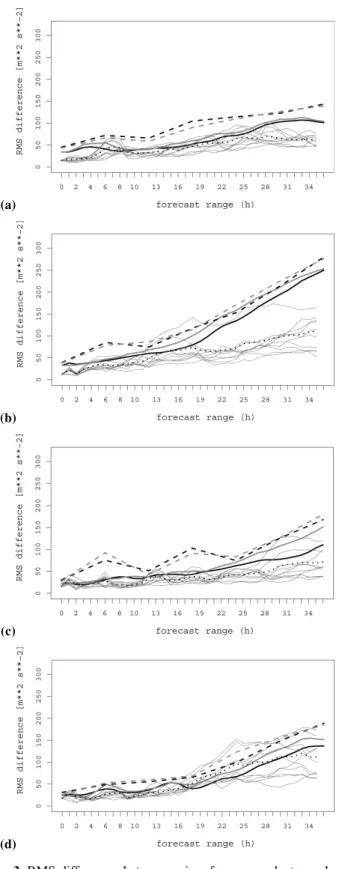
In order to check whether the direct nesting causes prob-lems in particular meteorological situations, error and spread have also been computed case by case. First, the RMS dif-ference between the geopotential field forecasted by each member of the COSMO-H2-EPS ensemble and by the cor-respondent member of the EXP-H2-EPS ensemble is com-puted. This is performed for each case separately, for each forecast hour (from 0 to 36 h) and over the whole integra-tion domain. RMS differences are shown in Fig. 3 as thin solid lines, while the thick dotted line is the average RMS difference, computed between all pairs of members. Results are shown for 4 cases only, selected as representative of the whole sample.
In order to provide a reference against which to evaluate the magnitude of these differences, the spread of the two en-sembles has also been computed for each case. The spread is regarded as a measure of the uncertainty expressed by each ensemble. Therefore a difference between pairs of members smaller than the spread would not be detected in the stan-dard ensemble configuration. The spread is plotted as thick solid lines, black for COSMO-H2-EPS and grey for EXP-H2-EPS. Finally, the RMSE of the ensemble mean is also computed for each case, and it is shown in Fig. 3 as a dashed line, black for COSMO-H2-EPS and grey for EXP-H2-EPS. RMSE provides the ultimate limit for the RMS differences between pairs of members, since it quantifies the error of the ensemble: until the difference induced by the different nest-ing approach is smaller than the error of the ensemble, it is not actually possible to establish if this difference is detri-mental to the forecast.
In all cases, the spread of each ensemble generally lies among the larger RMS differences between pairs of members and is larger than the average RMS difference. This indicates that the variability introduced by nesting the 2.8 km model on ENS directly is usually included within the uncertainty de-scribed by the reference ensemble (COSMO-H2-EPS). Fur-thermore, the RMS differences between pairs of members are generally smaller than the RMS error of the ensemble mean, with the few exceptions discussed below. This indicates that in most cases the impact of the different nesting is lower than the forecast error of the reference system.
Nevertheless, some differences can also be identified. The behaviour of the major part of cases (15 cases) is close to the one shown in Fig. 3a, relative to the 2012092512 case. The spread is smaller than the error of the ensemble mean for both ensembles, the two spread curves remaining quite close together for the entire forecast range. The differences between pairs of members are generally small, and do not give rise to additional uncertainty with respect to that rep-resented by the COSMO-H2-EPS ensemble. In a few cases among these 15, the RMS differences can increase up to the level of the RMSE for a few hours during the forecast range.
(a)
(b)
(c)
(d)
Fig. 3.RMS differences between pairs of correspondent members (thin solid), average RMS difference between all pairs (thick dot-ted), RMS spread (thick solid) and RMSE of the ensemble mean (thick dashed), as a function of the forecast range. RMS spread and error lines are black for COSMO-H2-EPS and grey for
EXP-H2-EPS. Plots are relative to four cases only: 2012092512 (a),
In the 2012101412 case (Fig. 3b), the spread increases quite sharply after 18–21 h of simulation, gaining distance from the RMS differences, which become negligible, with the exception of one pair of members. The spread curves roughly match the error curves. In this case, a trough enters the domain from the northwest corner after about 18 h of in-tegration. The z500 field forecasted by member 1 of EXP-H2-EPS (not shown) reproduces the observed trough and its evolution quite well, at difference with the corresponding member of COSMO-H2-EPS. The other pairs of members do not differ that much, but provide less skillful predictions. In the 2012102512 case (Fig. 3c), the RMS differences be-tween members are generally smaller than the spread and quite below the RMSE values. Also in this case, a marked spread increase is observed for EXP-H2-EPS after 20 h, lead-ing to a better match to the RMSE. The meteorological sit-uation is similar to the previous one, with one member of EXP-H2-EPS performing better than the others and better than the corresponding COSMO-H2-EPS member. In both the 2012101412 and 2012102512 cases, additional spread is gained with the direct nesting approach, with almost no in-crease in the RMSE, mainly due to the better performance of one EXP-H2-EPS member. A similar feature has been de-tected in two other cases (not shown).
The 2012103012 case (Fig. 3d) offers the most notable exception to the behaviour identified so far. The spread in-creases with the forecast range, especially after 18 h, in agreement with the increase in the forecast error. Never-theless, some members have differences larger than the en-semble spread, so that the variability introduced by the di-rect nesting can be detected as an “outlier” with respect to the variability described by the COSMO-H2-EPS ensemble. Furthermore, two pairs of members have differences larger than the RMSE. Since the RMSE of EXP-H2-EPS is higher that the RMSE of COSMO-H2-EPS, it is concluded that for this case additional error is introduced by the direct nest-ing. In this case, a deep low-pressure system over the west-ern Mediterranean develops and enters the domain approx-imately at the 18 h forecast range. Three members of EXP-H2-EPS provide a poor description of the position and inten-sity of the low, unlike the correspondent COSMO-H2-EPS members. For the other ensemble members, differences are smaller. Similar behaviour is found on the following day, for the 2012103112 case (not shown).
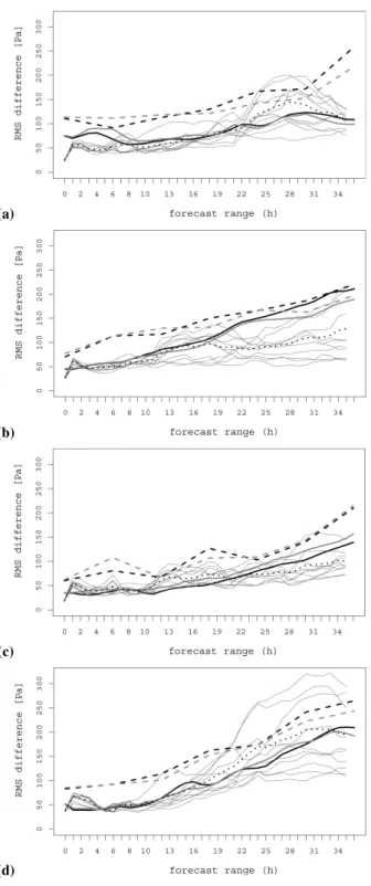
The same analysis has also been performed in terms of mean sea level pressure (Fig. 4), in order to assess the ro-bustness of the previous analysis.
Results are generally in good agreement with those ob-tained in terms of geopotential at 500 hPa. In the 2012092512 case (Fig. 4a), few RMS differences reach values close to or even above the RMSE. For most of the cases similar to this, though, RMS differences are well below these values. In the 2012103012 case (Fig. 4d), RMS differences of a few pairs of members are also quite high in terms of MSLP, confirming
(a)
(b)
(c)
(d)
Fig. 4.The same as in Fig. 3 but for mean sea level pressure.
the problem already detected in terms of z500 and ascribed to the evolution of the deep low-pressure system.
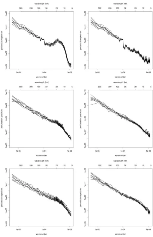
Fig. 5.Perturbation spectra of the field of geopotential at 500 hPa for each member of COSMO-H2-EPS (left panels) and EXP-H2-EPS (right panels) at the initial time (top), and at +6 h (middle) and +12 h (bottom) forecast range.
Initial state perturbations come, for both ensembles, from the ENS perturbed analyses, to which only the effect of the interpolation is added (Fig. 5, top panels). It is recalled here that the initial conditions of EXP-H2-EPS are directly inter-polated from the ECMWF ENS ones, from a 0.25 to 0.025 degree grid, while the initial conditions of COSMO-H2-EPS are interpolated from the COSMO-LEPS initial conditions,
all the larger-scale signals. For smaller scales, the spectra behave quite differently. With the direct interpolation (top right), perturbation amplitude is low on scales smaller than 60 km. The magnitude of the perturbations decreases quite steadily, with some noise especially at the wavelengths be-tween 10 and 5 km, close to the resolution of the 2.8 km grid. However, with the intermediate step (top left) there is a peak of magnitude in the perturbations at wavelengths between 20 and 10 km, approximately at the scale resolved by the 7 km model, followed by a sharp decrease and with little signal on the smaller scales. The peak at the 20–10 km wavelength is the part of the perturbations introduced by the interpola-tion on the 7 km grid. After 6 h of forecast (middle panels), the difference between the two spectra are significantly re-duced, both at the 20–10 and 10–5 km scale. The two spectra become quite similar after 12 h (bottom panels), both being characterised by a decrease in the perturbation magnitude for wavelengths below 10 km. Therefore the geopotential pertur-bations behave similarly from the point of view of how the signal propagates at the different scales. Similar behaviour has been detected for the other cases (not shown).
3.2 Analysis of the precipitation fields
The impact of the different nesting approaches on the precip-itation forecast is first evaluated by analysing the precipita-tion patterns, then by performing an objective verificaprecipita-tion of the ensemble performances against observations.
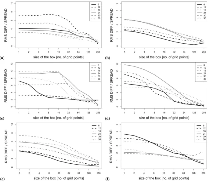
The difference between 6-hourly precipitation fields fore-casted by the members of COSMO-H2-EPS and of EXP-H2-EPS has been computed, summing up the RMS differ-ences between pairs of members. This computation has been performed at first on the original grid, then it has been re-peated after an upscaling of the fields over boxes which con-tain an increasing number of grid points: 2×2, 4×4, . . ., up to 256×256 points. Finally, the RMS difference has been divided by the spread of the COSMO-H2-EPS ensemble, to provide an indication of its significance with respect to the variability of the reference ensemble. Computation has been performed for each case and for each forecast range sepa-rately. In Fig. 6 the ratio between RMS difference and spread is shown for six cases, as a function of the horizontal scale of upscaling, for forecast ranges from 0–6 up to 30–36 h. It should be noted that the vertical scale is not the same in all the plots. This choice has been made to improve readability and should not affect the analysis of the results, since, as de-scribed, RMS difference is normalised by the correspondent spread. In order to identify the scale characterising the differ-ence in the precipitation patterns, the curve decrease is anal-ysed: a marked decrease in the curve (referred to as a “knee” in the curve) indicates which level of upscaling is needed to make the precipitation patterns significantly more similar to each other, compared with the spread of the ensemble. This level of upscaling, expressed in km of the upscaling box, de-tects the minimum spatial scale of the differences. When it
is not possible to find a “knee”, the scale at which the ra-tio between RMS difference and spread halves is adopted as a quantitative indicator of the scale of the differences. Here only 6 cases are shown, selected in order to represent the full spectrum of different behaviours of the 21 cases.
For the 2012092512 case (Fig. 6a), the differences are quite constant up to a horizontal scale of 8×8 grid points, then they start to decrease. A more marked decrease takes place for most forecast ranges at scales between 16 and 32 grid points. Therefore, the precipitation patterns fore-casted by the two systems have a minimum scale of differ-ences of the order of 24 km, but differdiffer-ences remain relatively high up to 90 km.
For the 2012093012 case (Fig. 6b), different behaviour is detected. The differences decrease quite steadily from the be-ginning, with a more marked decrease starting from the 4x4 grid point scale. Therefore, it is difficult to detect a minimum scale for the differences. The scale at which the ratio halves with respect to its original value is around 32×32 grid points, therefore about 90 km.
For the 201210612 case (Fig. 6c), the curves behave sim-ilarly to those of the first case. For all the forecast ranges a sharp decrease is observed, either at 16×16 or 32×32 grid point scale. Therefore, the minimum scale of the differences is in the order of 45 or 90 km, depending on the range consid-ered. The 6 h forecast range should not be considered, since only very light and localised precipitation was forecast and observed.
For the 2012101712 case (Fig. 6d), the behaviour is inter-mediate: the curves decrease already from the beginning, but the decrease is faster than for the 2012093012 case. The scale at which the ratio halves is between 16 and 32 grid points (45 and 90 km) for most of the forecast ranges, reducing to about 24 km only for the 12 h forecast range.
For the 2012102212 case (Fig. 6e), the curve decrease is initially very slow, then more pronounced. The scale at which the ratio halves is quite large, about 64 points (180 km) for the forecast ranges 18, 24, and 30 h, while it is smaller for the 12 (about 90 km) and 6 (about 45 km) h forecast range.
Finally, the 2012103012 case (Fig. 6f) has behaviour sim-ilar to that of the 2012101712 case for the first 4 forecast ranges: the curves decrease quite rapidly, especially from the 8×8 grid point scale, reaching values of half the initial ratio at scales between 45 and 90 km.
(a) (b)
(c) (d)
(e) (f)
Fig. 6.Ratio between the RMS difference between all the members of the two ensembles and the spread of COSMO-H2-EPS as a function of the horizontal scale of upscaling (indicated as the size, in grid points, of each upscaling box) in terms of 6 h accumulated precipitation for the different forecast ranges (from 0–6 to 30–36 h). Plots are for the cases (from top left to bottom right): 2012092512, 2012093012, 2012101612, 2012101712, 2012102212, 2012103012.
precipitation patterns forecasted by pairs of members is not negligible, even if in some cases it might be difficult to de-tect it properly with a synop observation network. It is not possible to draw conclusions about the influence of the fore-cast range, since the cases have been examined separately, and precipitation forecast in the different ranges is actually mainly dependent on the evolution of the phenomenon rather than on the forecast range itself.
Since differences are not negligible, an objective verifica-tion has also been performed, in order to assess the quality of the precipitation forecasts issued by the two ensembles. The verification period extends from 25 September to 6 Novem-ber 2012. As already mentioned, the experimental ensemble has only been run for 21 cases in this period, with a 36 h
forecast range. Therefore, the verification sample is slightly smaller than 1 month.
Verification was first performed over the entire domain, in terms of precipitation accumulated over 12 h compared against synop observations (about 400 stations in the do-main), considering the forecast value at the nearest grid point for each observation location.
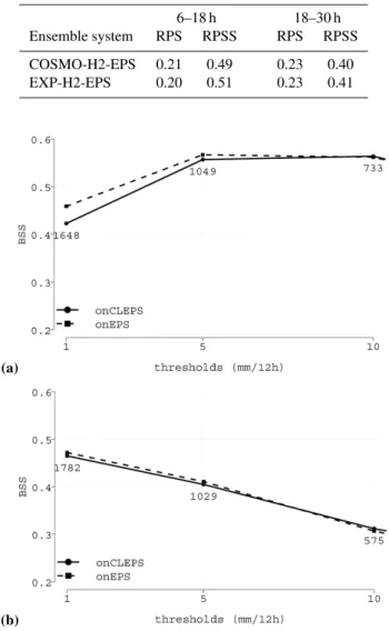
In Table 1 the values of the ranked probability score (RPS) and skill score (RPSS) are shown for each system and for each forecast range (6–18 and 18–30 h). The skill of the two ensembles is comparable, with a little outperformance of EXP-H2-EPS over COSMO-H2-EPS.
Table 1.Ranked probability score and skill score of the two ensem-bles computed in terms of 12 h accumulated precipitation against SYNOP data.
6–18 h 18–30 h
Ensemble system RPS RPSS RPS RPSS
COSMO-H2-EPS 0.21 0.49 0.23 0.40
EXP-H2-EPS 0.20 0.51 0.23 0.41
(a)
(b)
Fig. 7.Brier skill score of COSMO-H2-EPS (solid line, labelled “onCLEPS”) and EXP-H2-EPS (dashed line, labelled “onEPS”) as
a function of the threshold for the 6–18 h(a)and 18–30 h(b)
fore-cast range. Verification is performed for 12-hourly precipitation. Numbers indicate the observed occurrences of each event.
EXP-H2-EPS outperforming COSMO-H2-EPS for light pre-cipitation at the first forecast range (6–18 h). The number of events for each threshold is also reported in the plots.
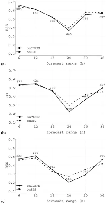
Since some heavy precipitation events took place over northern and central Italy during the analysed period, a dif-ferent verification has also been performed, aimed at evalu-ating the impact of the LBC diversity focussing on intense precipitation cases. Precipitation accumulated over 6 h has been considered and scores have been computed against ob-servations collected by a dense network covering northern and central Italy (about 850 stations). In order to perform a verification more suitable for high-resolution forecast of in-tense events, a different methodology has been adopted,
con-(a)
(b)
Fig. 8. Ranked probability score (a) and skill score (b) of COSMO-H2-EPS (solid line, labelled “onCLEPS”) and EXP-H2-EPS (dashed line, labelled “onEXP-H2-EPS”) as a function of the fore-cast range. Verification is performed for 6-hourly precipitation over northern and central Italy.
sisting in an upscaling of both forecast and observed values (Marsigli et al., 2008). The verification area has been cov-ered with boxes of 0.2 degrees×0.2 degrees, then the aver-ages (one for each member) of the values forecasted on the grid points falling in each box are compared with the average of the values observed on the stations falling in the same box, provided that a box contains at least 3 stations.
Both RPS and RPSS indicate that the skill of the two en-sembles is comparable (Fig. 8), EXP-H2-EPS slightly out-performing COSMO-H2-EPS at the 24 and 30 h forecast ranges. This dependence on the forecast range is ascribed to the performance of the two systems over a few intense events, which took place at these ranges, rather than on the forecast range itself. In order to check the dependency on the precip-itation intensity, the Brier skill score is also shown, for the 1, 5, and 10 mm thresholds (Fig. 9).
(a)
(b)
(c)
Fig. 9.The same as in Fig. 8 but for the Brier skill score. Thresholds
are: 1 mm(a), 5 mm(b), and 10 mm(c).
4 Summary and conclusions
An analysis has been undertaken of the performance of two different nesting approaches for convection-permitting en-semble forecasting. The reference approach, adopted in the COSMO-H2-EPS ensemble, consists of providing ICs and LBCs to the 2.8 km ensemble by a coarser-resolution ensem-ble based on the same model. The experimental approach, implemented in the EXP-H2-EPS ensemble, is a direct nest-ing, where ICs and LBCs are provided by a global ensem-ble, run at quite coarser resolution. The purpose of this work was to investigate the effect of the direct nesting approach,
compared with the one based on the intermediate step, for a specific application, which is ensemble forecasting over Italy with the main focus on the forecast of intense precipi-tation. Analysis has been performed in terms of geopotential at 500 hPa and precipitation.
Results show that the variability introduced in the geopo-tential fields by the direct nesting is often smaller than the uncertainty described by the reference ensemble, represented by the ensemble spread. When the forecast error is consid-ered, expressed by the RMSE of the ensemble mean, it ap-pears that the differences between pairs of members having different nesting approaches are generally smaller than this error, therefore hardly detectable from ensemble forecasting evaluation. A case study-based evaluation highlights that few cases show a different behaviour. In four cases the exper-imental nesting approach leads to a better performance of the ensemble, due to the better performance of one member. Nevertheless, in two other cases, an additional error is in-troduced on two ensemble members with the direct nesting. These results are confirmed by a similar analysis carried out in terms of mean sea level pressure.
Considering the relation between spread and error over the whole sample, it is found that the direct nesting leads to an improved relation, with spread slightly increased and error significantly reduced.
An analysis of the perturbation spectra indicates that the geopotential perturbations behave similarly in the two ap-proaches, from the point of view of the way the signal prop-agates at the different scales. Both ensembles are charac-terised by little signal on the small scales at initial time, as expected since ICs are downscaled from analyses perturbed at coarse resolution. Nevertheless, this feature will not af-fect the 2.8 km ensemble in its operational set-up, since high-resolution perturbed analyses derived from KENDA will be used as ICs.
In terms of precipitation, it is found that forecasts issued by members with different nesting approaches generally dif-fer on spatial scales which are highly dependent on the case, ranging from 16 up to 180 km. Though these differences are not negligible, it might be difficult to evaluate their impact on the forecast quality, since spatial errors in the precipita-tion fields may reach scales of 50–100 km even if forecasted by a high-resolution model.
This work should be regarded as the first step of a deeper analysis, where more cases will be considered, especially cluding different weather situations. Furthermore, it is in-tended to study the impact of spatial and temporal resolu-tion separately, considering the usefulness of hourly bound-ary conditions provided by the global ensemble.
Acknowledgements. This work was partly supported by the Italian Civil Protection Department, in the framework of the MODMDET3 Project. The Italian institutions providing observed precipitation data are also acknowledged. The authors are grateful to Jun Du and to two anonymous referees for their valuable comments, which allowed them to improve the manuscript greatly.
Edited by: R. Buizza
Reviewed by: J. Du and two anonymous referees
References
Amengual, A., Romero, R., Homar, V., Ramis, C., and Alonso, S.: Impact of the lateral boundary conditions resolution on dynam-ical downscaling of precipitation in mediterranean Spain, Clim. Dynam., 29, 487–499, doi:10.1007/s00382-007-0242-0, 2007. Buizza, R., Houtekamer, P. L.,Toth, Z.,Pellerin, G., Wei, M., and
Zhu, Y.: A Comparison of the ECMWF, MSC, and NCEP Global Ensemble Prediction Systems, Mon. Weather Rev., 133, 1076– 1097, 2005.
Davies, T.: Lateral boundary conditions for limited-area models, Q. J. Roy. Meteor. Soc., 140, 185–196, doi:10.1002/qj.2127, 2014. de Elia, R., Laprise, R., and Denis, B.: Forecasting skill limits
of nested, limited-area models: a perfect-model approach, Mon. Weather Rev., 130, 2006–2023, 2002.
Denis, B., Laprise, R., Côté, J., and Caya, D.: Downscaling abil-ity of one-way nested regional climate models: The big-brother experiment, Clim. Dynam., 18, 627–646, 2001.
Ducrocq, V., Braud, I., Davolio, S., Ferretti, R., Flamant, C., Jansa, A., Kalthoff, N., Richard, E., Taupier-Letage, I., Ayral, P.-A., Belamari, S., Berne, A., Borga, M., Boudevillain, B., Bock, O., Boichard, J.-L., Bouin, M.-N., Bousquet, O., Bouvier, C., Chig-giato, J., Cimini, D., Corsmeier, U., Coppola, L., Cocquerez, P., Defer, E., Delanoë, J., Di Girolamo, P., Doerenbecher, A., Drobinski, P., Dufournet, Y., Fourrié, N., Gourley, J. J., Labatut, L., Lambert, D., Le Coz, J., Marzano, F. S., Molinié, G., Mon-tani, A., Nord, G., Nuret, M., Ramage, K., Rison, B., Roussot, O., Said, F., Schwarzenboeck, A., Testor, P., Van Baelen, J., Vin-cendon, B., Aran, M., and Tamayo, J.: HyMeX-SOP1, the field campaign dedicated to heavy precipitation and flash flooding in the northwestern Mediterranean, B. Am. Meteorol. Soc., online first, doi:10.1175/BAMS-D-12-00244.1, 2013.
Ferretti, R., Pichelli, E., Gentile, S., Maiello, I., Cimini, D., Davo-lio, S., Miglietta, M. M., Panegrossi, G., Baldini, L., Pasi, F., Marzano, F. S., Zinzi, A., Mariani, S., Casaioli, M., Bartolini, G., Loglisci, N., Montani, A., Marsigli, C., Manzato, A., Pucillo, A., Ferrario, M. E., Colaiuda, V., and Rotunno, R.: Overview of the first HyMeX Special Observation Period over Italy: obser-vations and model results, Hydrol. Earth Syst. Sci. Discuss., 10, 11643–11710, doi:10.5194/hessd-10-11643-2013, 2013.
Gerard, L., Piriou, J.-M., Brožková, R., Geleyn, J.-F., and Banciu D.: Cloud and Precipitation Parameterization in a Meso-Gamma-Scale Operational Weather Prediction Model, Mon. Weather Rev., 137, 3960–3977, 2009.
HYMEX – HYdrological cycle in the Mediterranean EXperi-ment, Hymex Project, available at: www.hymex.org, last access: 4 March 2014, 2010–2020.
Marsigli, C., Montani, A., Nerozzi, F., Paccagnella, T., Tibaldi, S., Molteni, F., and Buizza, R.: A strategy for High–Resolution Ensemble Prediction. Part II: Limited–area experiments in four Alpine flood events, Q. J. Roy. Meteor. Soc., 127, 2095–2115, 2001.
Marsigli, C., Montani, A., and Paccagnella, T.: A spatial verifica-tion method applied to the evaluaverifica-tion of high–resoluverifica-tion ensem-ble forecasts, Meteorol. Appl., 15, 125–143, 2008.
Marsigli, C., Montani, A., and Paccagnella, T., 2013. Test of a COSMO-based convection-permitting ensemble in the Hymex framework, COSMO Newsletter No. 13, available at: http://www.cosmo-model.org/content/model/documentation/ newsLetters/default.htm, last access: 4 March 2014, 2013 Molteni, F., Buizza, R., Marsigli, C., Montani, A., Nerozzi, F., and
Paccagnella, T.: A strategy for High–Resolution Ensemble Pre-diction. Part I: Definition of Representative Members and Global Model Experiments, Q. J. Roy. Meteor. Soc., 127, 2069–2094, 2001.
Montani, A., Cesari, D., Marsigli, C., and Paccagnella, T.: Seven years of activity in the field of mesoscale ensemble forecasting by the COSMO-LEPS system: main achievements and open chal-lenges, Tellus A, 63, 605–624, 2011.
Nutter, P., Stensrud, D., and Xue, M.: Effects of coarsely resolved and temporally interpolated lateral boundary conditions on the dispersion of limited-area ensemble forecasts, Mon. Weather Rev., 132, 2358–2377, 2004.
Reich, H., Rhodin, A., and Schraff, C.: LETKF for the nonhy-drostatic regional model COSMO-DE, COSMO Newsletter No. 11, available at: http://www.cosmo-model.org/content/model/ documentation/newsLetters/default.htm, last access: 4 March 2014, 2011.
Steppeler, J., Doms, G., Schattler, U., Bitzer, H. W., Gassmann, A., Damrath, U., and Gregoric, G.: Meso-gamma scale forecasts us-ing the nonhydrostatic model LM, Meteorol. Atmos. Phys., 82, 75–96, 2003.
Termonia, P.: Monitoring and improving the temporal interpolation of lateral-boundary coupling data for limited-area models, Mon. Weather Rev., 131, 2450–2463, 2003.
Termonia, P., Deckmyn, A., and Hamdi, R.: Study of the lateral boundary condition temporal resolution problem and a proposed solution by means of boundary error restarts, Mon. Weather Rev., 137, 3551–3566, 2009.