Article
J. Braz. Chem. Soc., Vol. 22, No. 2, 327-336, 2011. Printed in Brazil - ©2011 Sociedade Brasileira de Química
0103 - 5053 $6.00+0.00
A
*e-mail: [email protected]
Elemental Analysis of Wines from South America and their Classiication
According to Country
Fabrina R. S. Bentlin,a Fernando H. Pulgati,b Valderi L. Dresslerc and Dirce Pozebon*,a
aInstituto de Química and bInstituto de Matemática, Universidade Federal do Rio Grande do Sul,
Av. Bento Gonçalves 9500, 91501-970 Porto Alegre-RS, Brazil
cDepartamento de Química, Universidade Federal de Santa Maria,
97105-900 Santa Maria-RS, Brazil
Elementos majoritários, minoritários e traço em vinhos provenientes de países produtores na América do Sul (Argentina, Brasil, Chile e Uruguai) foram determinados. A espectrometria de emissão óptica com plasma indutivamente acoplado (ICP OES) e a espectrometria de massa com plasma indutivamente acoplado (ICP-MS) em conjunto com nebulização pneumática e/ou nebulização ultra-sônica foram utilizadas. Foram determinados 45 elementos (Al, Ag, As, Ba, Be, Bi, Ca, Cd, Ce, Co, Cr, Cu, Dy, Er, Eu, Fe, Gd, Ho, K, La, Li, Lu, Mg, Mn, Mo, Na, Nd, Ni, P, Pb, Pr, Rb, Sb, Sn, Se, Sm, Sr, Tb, Ti, Tl, Tm, U, V, Yb e Zn) em 53 vinhos tintos. Mediante análise multivariada, os vinhos puderam ser discriminados de acordo com o país de origem, independentemente do tipo da uva. Os elementos discriminantes foram Tl, U, Li, Rb e Mg.
Major, minor and trace elements in wines from wine-producing countries in South America (Argentina, Brazil, Chile, and Uruguay) were determined. Inductively coupled plasma optical emission spectrometry (ICP OES) and inductively coupled plasma mass spectrometry (ICP-MS) combined with pneumatic and/or ultrasonic nebulization were used. The concentrations of 45 elements (Al, Ag, As, Ba, Be, Bi, Ca, Cd, Ce, Co, Cr, Cu, Dy, Er, Eu, Fe, Gd, Ho, K, La, Li, Lu, Mg, Mn, Mo, Na, Nd, Ni, P, Pb, Pr, Rb, Sb, Sn, Se, Sm, Sr, Tb, Ti, Tl, Tm, U, V, Yb, and Zn) in 53 red wines were determined. By means of multivariate analysis, the wines could be discriminated according to the country of origin, regardless of the type of grape. The discriminant elements were Tl, U, Li, Rb, and Mg.
Keywords: red wine provenance, multivariate analysis, element concentration, ICP OES, ICP-MS
Introduction
Wine has a long history dating back to biblical times. With the evolution of the viticulture, a wide sort of wines became available to consumers due to the varieties of grape grown and different methods of wine producing.
Several elements (especially Cd, Cu, Fe, Mn, Sn and Zn) when present in excessively high concentration in wines, adversely affect the organoleptic quality and the stability of the wine. They may cause a metallic taste, undesired color change or give rise to obstinate hazing and cloudiness.1 The
concentration of some elements can be a sort of ingerprint of the wine. The element proile does not depend exclusively
on the geochemistry of the provenance soil but is affected by the winemaking process and the grape variety. Identifying the origin of wine is of great interest to producers and consumers, as it provides criteria for deciding about the quality of wine. Therefore, a method for verifying authenticity is an essential requirement to control the product origin claims.
Studies have shown that the concentration proile of elements can be used to identify the provenance of a wine as well as its authenticity. 2-6 Lanthanides have been suggested
as a ingerprint for the provenance of wines.2,4 However,
caution must be taken because contamination may occur at the production step, transport and storage, as well as by inadequate winemaking practices.7,8
most appropriate techniques for the determination of trace elements in wine.9 However, the formation of molecular
species in the plasma, such as Ar2+, ArO+, ArN+, ArH+,
MAr+, ArX+ (M is a metal and X a non-metal) and other
polyatomic species (MO+, MOH+, XO+, XO
2+, XOH+) that
cause isobaric interferences may worsen precision and accuracy.10-12 Additionally, the formation of oxides can
also deteriorate the sensitivity for elements such as U, Ba and lanthanides.13,14 It is worth citing that the conditions
of operation of the instrument, the instrument type and quality of aerosol introduced into the plasma inluence the formation of molecular species. The use of nebulizers in conjunction with desolvation systems is a simple and effective way to decrease the formation of O and H interfering species, since most of the water is removed before the introduction of the sample solution into the plasma. Thus, the formation of oxide and hydroxides ions is drastically reduced.12,15 In addition, the limits of detection
(LODs) are better (typically in one order of magnitude) because more sample is transported to the plasma.14 With
the introduction of dry aerosol, the plasma is also more stable and consequently precision is improved. Molecular species of Ar and N interfere in the determination of Al, As, Se, Fe, K, Ca and Mg.14-16 These elements can be better
determined by using a double focusing sector ield mass spectrometer17 or ICP OES (in the case of Al, Fe, K, Ca and
Mg). Another way to minimize interferences by polyatomic ions in ICP-MS is the use of electrothermal vaporization (ETV) for introducing the sample into the plasma.18,19
However, elements such as B, Mo,20 lanthanides and
actinides produce thermally stable carbides in the graphite tube, increasing the LODs.
Due to the high content of organic compounds in wine, pretreatment of the sample is preferable for element determination by ICP OES and ICP-MS. The most common sample preparation procedure used is wet acid digestion or simple dilution of the sample. Although simple dilution is faster, not all investigated elements in the wine sample can be correctly determined in this way.
Studies to identify the origin of wines have already been published,2-6, 21,22 but none of them compared wines
from different countries of South America. Therefore, the main goal of this study was to develop a method for identifying the origin of red wines produced in Argentina, Brazil, Chile and Uruguay (the wine-producing countries in South America) by the concentration of major, minor and trace elements. The data was statistically processed by multivariate analysis in an attempt to identify the country of origin of the analyzed wines. A set of 45 elements was investigated in order to ind those that would better discriminate the wines.
Different procedures of sample treatment are evaluated in order to achieve good precision and accuracy of the results.
Experimental
Instrumentation
Major and minor elements (Al, Ba, Ca, Fe, K, Mg, Mn, Na, P, Rb, Sr, Ti, and Zn) were determined by using an Optima 2000 DV ICP OES spectrometer (Perkin-Elmer, Shelton, CT, USA). The following spectral lines (wavelength in nm) were monitored: Al (396.153), Ba (233.527), Ca (317.933), Fe (238.204), K (766.490), Mg (285.213), Mn (257.610), Na (589.592), P (213.617), Rb (780.023), Sr (407.771), Ti (334.940) and Zn (206.200). A pneumatic nebulizer itted to a cyclonic spray chamber was used for introducing the sample solution into the plasma. An ELAN DRC II instrument (from PerkinElmer/ SCIEX, Thornhill, Canada) was employed for minor and trace elements determination. Instrumental parameters (using the ICP-MS instrument in standard mode) such as the nebulizer gas low rate, RF power and lens voltage were optimized in order to obtain the maximum intensity of 115In+ and minimum intensity of Ba++/Ba+ and LaO+/La+.
The following isotopes were monitored: 7Li, 9Be, 51V, 53Cr, 58Ni, 59Co, 65Cu, 75As, 82Se, 98Mo, 107Ag, 111Cd, 120Sn, 121Sb, 205Tl, 208Pb, 209Bi, 238U, 139La, 140Ce, 141Pr, 146Nd, 147Sm, 151Eu, 157Gd, 159Tb, 163Dy, 165Ho, 167Er, 169Tm, 172Yb, and 175Lu.
An ultrasonic nebulizer was used for the determination of Be, Ag, Cd, Sn, Sb, Tl, Bi, U, La, Ce, Pr, Nd, Sm, Eu, Gd, Tb, Dy, Ho, Er, Tm, Yb, and Lu. The heating and cooling temperatures of the ultrasonic nebulizer were set at 140 °C and − 4 °C, respectively. A concentric nebulizer
(Meinhard®, Golden, CO, USA) itted to a cyclonic spray
chamber was used for the determination of Li, V, Cr, Ni, Co, Cu, As, Mo, Se, and Pb.
The spray chambers and MicroMist nebulizer used were from Glass Expansion (Melbourne, Australia), the ultrasonic nebulizer was from CETAC (Omaha, NE, USA), whereas the Meinhard nebulizer was from Meinhard Associates. The conditions established for the elements determination in the wine samples are summarized in Table 1. The SPSS 18.0 software was used for statistical analysis. Factorial, cluster and discriminant analysis were used.
Reagents and solutions
Nitric acid (from Merck, Darmstadt, Germany), puriied by distillation in sub-boiling quartz apparatus was used. High-purity water (resistivity of 18.2 MΩ cm) obtained
USA) was used for the preparation of all samples and solutions. Calibration solutions were prepared (in 5% v/v HNO3) from serial dilutions of 10 mg L-1 multielemental
stock solutions (Plasma Cal SCP33MS from SCP Science-Canada and CLMS-1 from SPEX, Metuchen, NJ, USA). The calibration solutions of P were prepared from a 1000 mg L-1
P stock solution (Titrisol/Merck). The calibration solutions concentration and techniques used for each group of elements are summarized in Table 2. The elements quantiication was assessed using external calibration.
Samples and sample preparation
Samples of red wine from different regions of the four wine-producing countries in South America (Argentina, Brazil, Chile and Uruguay) were purchased in local markets. The geographical origin and cultivars were given on the label of the wine bottle. The identiication of the analyzed samples is given in Table 3. Excepting Bordeaux and Isabella, the wines were produced from grapes of Vitis vinifera species (speciic for wine production). Assemblage is a type of wine produced by a blend of different grapes, unlike a varietal wine, which is made from only one grape and carrying the name of that grape. The blend of different grapes aims to add new lavors and aromas to the wine, leaving it more complex,
or soft, depending on the goal. For instance, wine-tasting tannins such as Tannat can be softened by addition of Merlot grape. Another example of combination of aromas and lavors is the blend of the grapes Shiraz (also named Syrah) and Cabernet Sauvignon. According to Table 3, the number of samples was not the same for each country because not all cultivars are produced in the four wine-producing countries in South America or not easily found in the market.
The wine samples were decomposed according to the following procedure: 1 mL of wine was transferred to polytetraluoroethylene (PTFE) lasks, to which 3 mL of HNO3 were added and the mixture let to stand for 15 h. Subsequently, the vessels were closed and heated in a metal block, in three steps: 50 °C for 1 h, 100 °C for 1 h and 150 °C for 3 h. After cooling, the obtained solution was transferred to graduated-polypropylene vial and the volume was made up to 25 mL with water. This solution was tenfold diluted with 5% v/v HNO3 for determinations by ICP OES, twofold diluted with 5% v/v HNO3 for determinations by ICP-MS or directly analyzed by ICP-MS. All samples were analyzed in triplicate.
Analyte recovery tests and comparison of results obtained by ICP-MS and ICP OES were used to evaluate possible interferences and check precision and accuracy. For evaluation of the sample preparation procedure, a red Table 1. Instrumental and optimized operating conditions
Parameter ICP OES ICP-MS
Pneumatic Nebulization Ultrasonic Nebulization
RF Power / W 1500 1200 1100
Plasma gas low rate / (L min-1) 15 15 15
Auxiliary gas low rate / (L min-1) 0.20 1.20 1.20
Nebulizer carrier gas low rate / (L min-1) 0.75 1.03 1.00
Sample uptake rate / (mL min-1) 0.75 1.2
-Nebulizer MicroMist MCN-600 Meinhard® type A US-5000 AT+
Background correction 2 points/peak -
-Spray chamber Cinnabar cyclonic unbafled Cinnabar cyclonic-bafled
-Injector tube alumina 2-mm id quartz 2-mm id
Table 2. Stock solutions, concentrations range of calibration curves and nebulizers used for the elements determination by ICP-MS and ICP OES
Stock Solution Element calibration curve / (Concentration range of
µg L-1) Technique/nebulizer
CLMS-1 La, Ce, Pr, Nd, Sm, Eu, Gd, Tb, Dy, Ho, Er, Tm, Yb and Lu
0.01-1.0 ICP-MS/ultrasonic
SCP 33MS Be, Se, Ag, Cd, Sn, Sb, Tl, Bi, U 0.01-1.0 ICP-MS/ultrasonic
SCP 33MS Li, V, Cr, Ni, Co, Cu, As, Mo and Pb 0.05-10 ICP-MS/Meinhard
SCP 33MS Al, Ba, Ca, Fe, K, Mg, Mn, Na, Rb, Sr, Ti and Zn 50-500 ICP OES/MicroMist ICP-MS/Meinhard
wine sample was simply diluted with nitric acid solution (to obtain 5% v/v HNO3) or left in contact with HNO3(1 mL of wine + 3 mL of HNO3) or decomposed as above described.
Results and Discussion
Chemical analysis
Wine is a complex matrix, producing spectral and non-spectral interferences in the plasma. Investigations were irstly carried out with respect to wine sample preparation, with the aim to analyze the wine samples directly (without
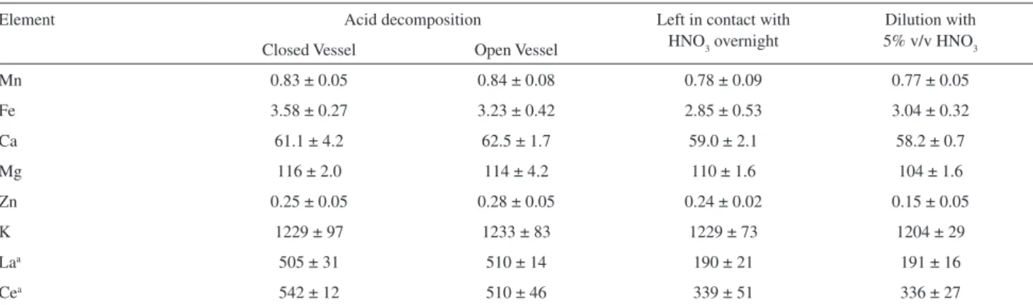
decomposition), which would simplify the work. The results obtained for some elements are presented in Table 4. It shows thatthe concentrations of the elements tend to be higher when the wine is decomposed with acid. With respect to major elements, there is no signiicant statistic difference (at 95% of conidence level, according to the t-student test) between the procedures of sample preparation, except for diluting the sample with nitric acid. However, the concentrations of La and Ce (trace elements) are different. Change of plasma characteristics due to the organic matrix loading can be one of the reasons for the lower results observed, and/or the residence time Table 3. Wine samples identiication
Country Grape Region Year Country Grape Region Year
Argentina Cabernet
Sauvignon
Salta 2006 Chile Cabernet
Sauvignon
Maipo 2007
Mendoza 2006 Colchagua 2003
Mendoza 2005 Curicó 2006
Malbec Mendoza 2008 Requinoa 2005
Mendoza 2007 Requinoa 2008
Mendoza 2007 Malbec Curicó 2005
Mendoza 2006 Aconcagua 2006
Mendoza 2005 Merlot Requinoa 2002
Merlot Mendoza 2008 Maipo 2007
Mendoza 2006 Racangua 2007
Shiraz Mendoza 2007 Carmenere Colchagua 2008
Pinot Noir Patagonia 2009 Shiraz Racangua 2007
Assemblage Mendoza 2002 Pinot Noir Requinoa 2008
Brazil Cabernet
Sauvignon
Bento Gonçalves/RS 2005 Uruguay Cabernet
Sauvignon
Montevideo 2006
Santana do Livramento/RS
2007 San José 2006
Farroupilha/RS 2009 Colonia 2007
Santa Maria/RS 2006 Canelones 2004
Santa Maria/RS 1999 Malbec Florida 2007
Malbec Bento Gonçalve/RS 2005 Merlot Colonia 2007
Bento Gonçalves/RS 2006 Florida 2007
Merlot Santana do
Livramento/RS
2008 Tannat Canelones 2007
Bento Gonçalves/RS 2006 Montevideo 2007
Bento Gonçalves/RS 2009 Canelones 2007
Pinot Noir Santana do
Livramento/RS
2007 Shiraz Artigas 2008
Shiraz Casa Nova/BA 2007 Pinot Noir Canelones 2008
Tannat Santana do
Livramento/RS
2007
Isabella Cotiporã/RS 2006
in the plasma is not suficient for all processes (matrix decomposition and analyte ionization). Some wine samples that were simply diluted were also analyzed by ICP-MS. In this case, the main problem observed was the enhancement of the signals of As and Se, probably due to the presence of carbon.23 On the other hand, progressive signal suppression
of other elements was observed, caused mainly by carbon deposits on the interface (cones, photon stop and lens) of the ICP-MS instrument. Therefore, according to the results obtained in this step of the work and keeping in mind the large number of elements to be determined by ICP-MS or ICP OES, the wine samples were acid digested.
Since there was no certiied wine available, the matrix inluence was investigated by means of recovery tests and/ or analyte determination by both ICP OES and ICP-MS. For the recovery tests, the solution of a digested sample (1 mL of wine was digested and the obtained solution diluted to 25 mL) was spiked with the elements of interest. As shown in Table 5, either analyte recovery was close to 100% or the results obtained by ICP-MS and ICP OES were in agreement (similar at 95% level, according to the t-student test).
As expected, the LODs improved and oxide formation rate reduced for a group of elements (Be, Ag, Cd, Sn, Sb, Tl, Bi, U, La, Ce, Pr, Nd, Sm, Eu, Gd, Tb, Dy, Ho, Er, Tm, Yb, and Lu) by using ultrasonic nebulization (a dessolvated aerosol is produced) for sample introduction into the plasma.11 However, Se could not be determined
by using ultrasonic nebulization due to signal instability (the relative standard deviation was higher than 30%). The instability of the signal is possibly due to heating and volatilization of Se in the ultrasonic nebulizer. Then, pneumatic nebulization was used for Se determination in all samples. With respect to major elements measured by ICP OES (K, P, Mg, Ca, and Na) no interferences were
observed. In this case, the digested sample solution was diluted at least 100 fold.
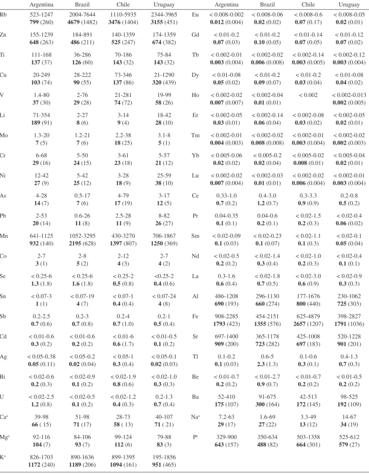
The concentrations of the investigated elements in the wine samples are summarized in Table 6 and Table S1 (Supplementary Information, SI). According to the results shown in these tables, the concentrations of most elements are heterogeneous within the samples. This may be caused not only by the soil type where the vines are grown, but also by the chemicals used as pesticides, winemaking processes and storage. It can be observed that the highest concentrations of V, Mo, As, Cd, Ag and Bi were found in wines from Chile; Rb, Tl, Mn, Be and Ba in wines from Brazil; Li and U in wines from Argentina; and Cu, Pb and Ni in wines from Uruguay. The concentrations of some elements in several samples are lower than the LODs. The LOD is the concentration equivalent to (B + 3s)fd, where B is the average concentration of ten consecutive measurements of the sample blank, s is the standard deviation of ten consecutive measurements of the same blank, and fd is the dilution factor of the wine sample (1 mL of wine diluted to 25 mL). Values lower than the LODs were treated by assuming the LOD values in the calculations of the means and standard deviations shown in Tables 6 and S1.
Statistical analysis
An exploratory analysis of the data was initially carried out. A Merlot wine from Chile was considered an extreme value and for that reason it was excluded. With respect to the other analyzed wines, only those obtained from grapes of Vitis vinifera strains were considered for multivariate analysis. Therefore, four wine samples were excluded from the multivariate analysis: one Merlot (from Chile) and the assemblage, Isabella and Bordeaux (see Table 3). Of the
Table 4. Elements determined (mg L-1) in red wine, as a function of different sample preparation procedures. Results are the average and standard deviation of triplicates
Element Acid decomposition Left in contact with
HNO3 overnight
Dilution with 5% v/v HNO3
Closed Vessel Open Vessel
Mn 0.83 ± 0.05 0.84 ± 0.08 0.78 ± 0.09 0.77 ± 0.05
Fe 3.58 ± 0.27 3.23 ± 0.42 2.85 ± 0.53 3.04 ± 0.32
Ca 61.1 ± 4.2 62.5 ± 1.7 59.0 ± 2.1 58.2 ± 0.7
Mg 116 ± 2.0 114 ± 4.2 110 ± 1.6 104 ± 1.6
Zn 0.25 ± 0.05 0.28 ± 0.05 0.24 ± 0.02 0.15 ± 0.05
K 1229 ± 97 1233 ± 83 1229 ± 73 1204 ± 29
Laa 505 ± 31 510 ± 14 190 ± 21 191 ± 16
Cea 542 ± 12 510 ± 46 339 ± 51 336 ± 27
Table 5. Recovery of the elements in a digested Cabernet Sauvignon wine
determined by ICP-MS or by two different techniques for Sr, Fe, Al, Ba, Mn, Rb, Sn, and Ti. Uncertainties are the standard deviations of triplicates
Element Concentration found in the sample / (µg L-1)
Added / (µg L-1)
Found / (µg L-1)
Recovery / %
Cu 52.8 ± 0.6 2.50 54.2 ± 0.4 98
V 6.44 ± 0.30 2.50 8.68 ± 0.25 97
Li 13.1 ± 2.9 2.50 15.5 ± 2.1 99
Mo 3.30 ± 0.41 2.50 5.69 ± 0.45 98
Cr 2.84 ± 015 2.50 5.51± 0.20 103
Ni 18.7 ± 1.3 2.50 20.8 ± 15 98
As 3.11 ± 0.36 2.50 5.50 ± 0.28 98
Pb 8.40 ± 0.34 2.50 11.1 ± 0.38 102
Co 2.50 ± 0.04 2.50 5.00 ± 0.06 100
Se < 0.25a 2.50 2.48 ± 0.10 99
Sn 15.2 ± 1.4 2.50 17.0 ± 1.2 96
Sb 0.249 ± 0.041 2.50 2.64 ± 0.03 96
Cd < 0.10 a 2.50 2.48 ± 0.12 99
Ag < 0.05 2.50 2.45 ± 0.01 98
Tl 4.12 ± 0.11 2.50 6.62 ± 0.14 100
Bi < 0.025a 2.50 2.48 ± 0.05 99
Be 0.930 ± 0.08 2.50 3.40 ± 0.08 99
U < 0.025 2.50 2.48 ± 0.02 99
La 0.610 ± 0.090 0.250 0.869 ± 0.070 101
Ce 0.800 ± 0.090 0.250 1.08 ± 0.027 103
Pr 0.201 ± 0.012 0.250 0.455 ± 0.040 101
Nd < 0.025a 0.250 0.247 ± 0.030 99
Sm 0.147 ± 0.013 0.250 0.389 ± 0.018 98
Eu 0.063 ± 0.034 0.250 0.307 ± 0.040 98
Gd 0.152 ± 0.034 0.250 0.410 ± 0.038 102
Tb 0.020 ± 0.004 0.250 0.267 ± 0.005 99
Dy 0.153 ± 0.031 0.250 0.399 ± 0.030 99
Ho 0.043 ± 0.008 0.250 0.293 ± 0.007 100
Er 0.139 ± 0.013 0.250 0.363 ± 0.016 101
Tm 0.022 ± 0.003 0.250 0.272 ± 0.005 100
Yb 0.153 ± 0.019 0.250 0.399 ± 0.023 99
Lu 0.024 ± 0.004 0.250 0.269 ± 0.005 99
ICP OES / (µg L-1) ICP-MS / (µg L-1)
Sr 570 ± 90 576 ± 121
Fe 1918 ± 75 1841 ± 53
Al 296 ± 27 302 ± 33
Ba 250 ± 10 240 ± 15
Mn 3232 ± 43 3167 ± 78
Rb 7644 ± 154 7338 ± 191
Zn 343 ± 22 333 ± 34
Ti 1145 ± 31 1123 ± 26
alimits of detection.
total of 45 variables (elements) ive of them (Mg, Li, Rb, U and Tl) were actually used after exploratory analysis of the data. Figure 1 shows the box-plot graphs related to these elements, showing the differences observed between the countries, which were signiicant according to the F test with sampling descriptive level of p < 0.001. According to Figure 1, three values of Rb are outliers, which were kept for the subsequent multivariate analysis. In this work, the outliers and extreme values were deined as those values whose distances from the nearest quartile were 1.5 and 3.0 times greater than the interquartile range, respectively.
Table 6. Concentrations range (µg L-1), means (in bold) and standard deviations (values in parenthesis) of minor and trace elements found in red wines. Number of samples: 13 from Argentina, 15 from Brazil, 13 from Chile, and 12 from Uruguay
Argentina Brazil Chile Uruguay Argentina Brazil Chile Uruguay
Rb 523-1247
799 (260)
2004-7644
4679 (1482)
1110-5935
3476 (1404)
2344-3965
3155 (451)
Eu < 0.008-0.002
0.012 (0.004)
< 0.008-0.06
0.02 (0.02)
< 0.008-0.6
0.07 (0.17)
< 0.008-0.05
0.02 (0.01)
Zn 155-1239
648 (263)
184-891
486 (211)
140-1359
525 (247)
174-1359
674 (382)
Gd < 0.01-0.2
0.07 (0.03)
< 0.01-0.2
0.10 (0.05)
< 0.01-0.14
0.07 (0.05)
< 0.01-0.12
0.07 (0.02)
Ti 111-168
137 (37)
36-286
126 (60)
70-186
143 (32)
75-84
143 (32)
Tb < 0.002-0.01
0.003 (0.004)
< 0.002-0.02
0.006 (0.008)
< 0.002-0.14
0.003 (0.005)
< 0.002-0.12
0.003 (0.004)
Cu 20-249
103 (74)
28-222
90 (55)
73-346
137 (86)
21-1290
320 (439)
Dy < 0.01-0.08
0.05 (0.02)
< 0.01-0.2
0.09 (0.07)
< 0.01-0.2
0.03 (0.04)
< 0.01-0.08
0.04 (0.02)
V 1.4-80
37 (30)
2-76
29 (28)
21-281
74 (72)
19-99
58 (26)
Ho < 0.002-0.02
0.007 (0.007)
< 0.002-0.04
0.01 (0.01)
< 0.002 < 0.002-0.013
0.002 (0.005)
Li 71-354
189 (91)
2-27
8 (6)
3-14
9 (4)
18-42
28 (10)
Er < 0.002-0.05
0.03 (0.01)
< 0.002-0.14
0.06 (0.04)
< 0.002-0.08
0.03 (0.02)
< 0.002-0.05
0.02 (0.01)
Mo 1.3-20
7 (5)
1.2-21
7 (6)
2.2-38
18 (25)
3.1-8
5 (1)
Tm < 0.002-0.01
0.004 (0.003)
< 0.002-0.02
0.008 (0.008)
< 0.002-0.01
0.003 (0.004)
< 0.002-0.02
0.002 (0.003)
Cr 6-68
29 (16)
5-50
24 (15)
3-61
23 (18)
5-57
21 (12)
Yb < 0.005-0.06
0.02 (0.02)
< 0.005-0.2
0.02 (0.04)
< 0.005-0.02
0.008 (0.01)
< 0.005-0.04
0.02 (0.01)
Ni 12-42
27 (9)
5-42
25 (12)
3-28
18 (9)
25-59
38 (10)
Lu < 0.002-0.02
0.007 (0.004)
< 0.002-0.03
0.01 (0.01)
< 0.002-0.02
0.006 (0.004)
< 0.002-0.01
0.003 (0.004)
As 4-28
14 (7)
0.5-17
7 (6)
4-79
17 (19)
3-17
12 (5)
Ce 0.33-1.0
0.7 (0.2)
0.4-3.0
1.2 (0.7)
0.3-3.3
0.9 (0.9)
0.2-0.8
0.5 (0.2)
Pb 2-53
20 (14)
0.6-26
11 (8)
2.5-28
11 (9)
8-82
26 (27)
Pr 0.04-0.35
0.1 (0.1)
0.04-0.6
0.2 (0.1)
< 0.02-1.5
0.2 (0.3)
< 0.02-0.4
0.06 (0.02)
Mn 641-1125
932 (140)
1052-3295
2195 (628)
430-3270
1397 (807)
706-1867
1250 (369)
Sm < 0.02-0.09
0.1 (0.03)
< 0.02-0.23
0.1 (0.07)
< 0.02-1.1
0.1 (0.3)
< 0.02-0.1
0.05 (0.04)
Co 2-7
3 (1)
2-8
5 (2)
2-12
4 (3)
2-7
4 (2)
Nd < 0.02-0.5
0.2 (0.2)
< 0.02-1.4
0.3 (0.4)
< 0.02-1.0
0.2 (0.3)
< 0.02-0.4
0.1 (0.1)
Se < 0.25-6
1.3 (1.8)
< 0.25-6
1.6 (1.8)
< 0.25-2
0.5 (0.8)
<0.25-2
0.4 (0.6)
La 0.3-1.6
0.6 (0.4)
< 0.02-1.8
0.7 (0.5)
< 0.02-3.0
0.6 (0.9)
< 0.02-0.9
0.3 (0.3)
Sn < 0.07-3
1 (1)
< 0.07-19
4 (7)
< 0.07-1
0.4 (0.4)
< 0.07-24
4 (8)
Al 486-1208
690 (193)
296-1130
660 (274)
177-1676
800 (440)
230-1062
725 (303)
Sb 0.2-2.5
0.7 (0.6)
0.2-3
0.7 (0.8)
0.2-4
0.7 (1.0)
0.2-1
0.5 (0.4)
Fe 908-2285
1793 (423)
454-2151
1355 (576)
625-4879
2657 (1207)
398-2827
1791 (1036)
Cd < 0.01-0.6
0.3 (0.2)
< 0.01-0.6
0.2 (0.2)
< 0.01-6
0.6 (1.7)
< 0.01-0.5
0.1 (0.2)
Sr 697-1400
909 (200)
365-1178
723 (282)
425-1008
697 (183)
520-1228
901 (201)
Ag < 0.05-0.38
0.05 (0.11)
< 0.05-0.2
0.02 (0.04)
< 0.05-1
0.3 (0.4)
< 0.05-0.1
0.02 (0.03)
Tl 0.1-0.2
0.1 (0.03)
0.6-5
2.3 (1.3)
0.1-0.6
0.3 (0.1)
0.4-1.3
0.7 (0.3)
Bi < 0.02-0.6
0.2 (0.3)
< 0.02-0.9
0.1 (0.2)
< 0.02-1.9
0.8 (0.6)
< 0.02-1.0
0.3 (0.3)
Be < 0.01-0.7
0.2 (0.2)
< 0.01-2.7
0.9 (0.7)
< 0.01-0.7
0.2 (0.2)
< 0.01-0.5
0.2 (0.2)
U < 0.02-2.5
1.2 (0.8)
< 0.02-0.5
0.1 (0.2)
< 0.02-1.2
0.4 (0.3)
0.2-1.3
0.7 (0.4)
Ba 52-410
175 (107)
91-675
300 (164)
42-513
172 (145)
98-525
192 (109)
Caa 39-98
66 ( 15)
51-98
71 (17)
28-73
58 ( 13)
40-107
71 ( 21)
Naa 7.2-63
29 (17)
1.6-69
27 (22)
3.3-49
13 (12)
14-67
34 (19)
Mga 92-116
104 (7)
84-106
93 (7)
99-124
112 (6)
79-88
83 (3)
Pa 329-900
643 (157)
350-634
488 (82)
503-1358
664 (301)
525-612
579 (27)
Ka 826-1703
1172 (240)
890-1636
1189 (206)
899-1395
1094 (161)
195-1856
951 (465)
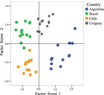
The result of cluster analysis is depicted in Figure 3, which highlights the similarity of the composition of the wines with respect to the elements shown in Figure 2. The similarity matrix was obtained using squared Euclidean, while distance and clustering were produced using the Ward’s method. Figure 3 shows strong evidence that the similarity observed is closely associated with the country of origin, since the resulting groups are primarily structured according to the origin. Excepting a Chilean wine (sample 34), classiied within the group dominated by Brazilian wines, all other observations (samples) follow a pattern of very high similarity within a country and extremely high dissimilarity between countries.
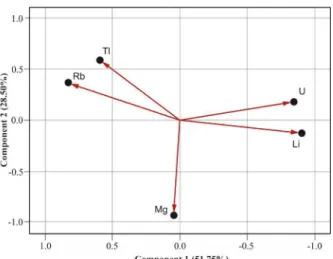
Figure 4 shows the dispersion of the scores of principal component analysis associated with each wine, with an indication of each group resulting from cluster analysis presented in Figure 3. By analyzing Figures 2 and 4 together it is observed that Li and U are higher in Argentinean wines in comparison to Brazilian and Chilean wines; Rb and Tl are higher in Brazilian and Chilean wines when compared with Argentinean wines; Mg is higher in Chilean and some Argentinean wines at the same time as it is lower in Uruguayan and some Brazilian wines.
In the second approach the discriminant model was employed, which considered the origin of the wines as the dependent variable and the ive elements previously identiied (Li, Mg, Rb, Tl and U) as the independent variable. The non-standardized coefficients for each canonical discriminant function (used to discriminate the ive countries as a function of the ive chemical elements) andthe correlation between discriminating variables and standardized discriminant function are presented in Table 7. The discriminant variables (B) show that Li and Rb are more correlated with function 1, Mg with functions 2 and 3, and Tl and U with function 3.
As a result, the centroids for each country were obtained; the dispersion among the scores from the discriminant functions 1 and 2 are shown in Figure 5. According to this igure, function 1 discriminates the samples from Argentina in a group and samples from Brazil and Chile in another group; function 2 discriminates the samples from Chile of those from Brazil and Uruguay; and function 3 discriminates the samples from Brazil of those from Uruguay.
Additionally, a cross validation text was performed. The results of classiication of cases revealed that the proposed model of classiication was successful in 100% of the cases and the results were 100% accurate.
Figure 2. Scatter plot of components 1 and 2 and respective loadings of Mg, Rb, Tl, U, and Li.
Conclusions
By multivariate analysis based on the concentration of chemical elements it was possible to discriminate red wines from the four wine-producing countries in South America according to country. Lithium, Mg, Rb, Tl, and U allowed discrimination of varietal red wines obtained from grapes of Vitis vinifera species. The type of yeast used, the way the vines are cultivated, knowledge of the winemaker that inluences the way of making wine, storage form, fertilizers and fungicides used may have contributed for the differences among the wines.
Although some authors have recommended that the lanthanides alone can distinguish wines,2,4 this strategy
was not feasible in the present work. The concentrations of these elements are very low in most wines from South America and not all of them were detected in several samples, despite using a highly sensitive technique (ICP-MS and ultrasonic nebulization for sample introduction into the plasma).
It was observed that the concentrations of some elements measured in red wine may be lower than the actual concentrations if the sample is simply diluted instead of being digested.
Supplementary Information
Supplementary data are available free of charge at http://jbcs.sbq.org.br, as PDF ile.
Acknowledgments
To CNPq for inancial support and CAPES for the scholarship of Fabrina R. S. Bentlin.
References
1. Detering, J.; Sanner, A.; Usnegger, B.; US pat 5,094,867 1992.
2. Galgano, F.; Favati, F.; Caruso, M.; Scarpa, T.; Palma, A.; Food Sci. Technol. 2008, 41, 1808.
3 Kment, P.; Mihaljevic, E. M. V.; Sebek, O.; Strnad, L.; Rohlová, L.; Food Chem. 2005, 91, 157.
4. Augagneur, S.; Médina, B.; Szpunar, J.; Lobinski, R.; J. Anal. At. Spectrom. 1996, 11,713.
5. Capron, X.; Smeyers-Verbeke, J.; Massart, D. L.; Food Chem.
2007, 101,1608.
6. Coetzee, P. P.; Steffens, F. E.; Eiselen, R. J.; Ockert, P. A.; Balcaen, L.; Vanhaecke, F.; J. Agric. Food Chem. 2005, 53,
5060.
7. Jakubowski, N.; Brandt, R.; Stuewer, D.; Schnauer, H. R.;
Görtges, S.; Fresenius J. Anal. Chem. 1999, 364, 424.
Figure 4. Scatter plot of the scores of the two principal component analysis of red wines (49 samples) from South America showing similarity within the country and dissimilarity between countries.
Figure 5. Scatter plot of the unstandardized canonical discriminant
functions 1 and 2 describing the countries of red wines (49) origin.
Table 7. Non-standardized coeficients of the canonical discriminant functions (A) and correlation between the discriminant function and the measured chemical element (B)
Variable
Function
1 2 3 1 2 3
A B
Mg −6.476 17.94 5.676 −0.041 0.639a 0.639a
Li 1.786 −0.492 −0.246 0.720a 0.111 0.019
Tl 0.148 −3.714 3.532 −0.255 0.450 0.651a
U 0.636 1.356 −0.613 0.235 0.035 −0.256a
Rb −1.913 0.413 −1.858 0.543a 0.253 −0.391
(Constant) 83.40 −206.3 −51.49 - -
-aLargest absolute correlation between each variable and the discriminant
8. Rossano, E. C.; Szilágyi, Z.; Malorni, A.; Pocsfalvi, G.; J. Agric. Food Chem. 2007, 55, 311.
9. Gonzálvez, A.; Llorens, A.; Cervera, M. L.; Armenta, S.; de la Guardia M.; Food Chem. 2009, 112, 26.
10. Longerich, H. P.; Fryer, B. J.; Strong, D. F.; Kantipuly, C. J.; Spectrochim. Acta, Part B 1987, 42, 75.
11. Tan, S. H.; Horlick. G.; Appl. Spectrosc. 1986, 40, 445. 12. Vanhoe, E. H.; Goosens, J.; Moens, L.; Richard, D.; J. Anal.
At. Spectrom. 1994, 9, 177.
13. Becker, J. S.; Inorganic Mass Spectrometry: Principles and Application; John Wiley and Sons: Chichester, 2007. 14. Dressler,V. L.; Pozebon, D.; Matusch, A.; Becker, J. S.; Int. J.
Mass Spectrom. 2007, 266, 25.
15. D’Ilio, S.; Violante, N.; Caime, S.; Gregório, D.; Petrucci, F.; Senofonte, O.; Anal. Chim. Acta 2006, 573, 432.
16. Pozebon, D.; Dressler, V. L.; Curtius, A. J.; At. Spectrosc. 1998,
19, 80.
17. Serapinas, P.; Venskutonis, P. R.; Aninkevi ius, V.; Ežerinskis, Ž.; Galdikas, A.; Juzikiene, V.; Food Chem. 2008, 107, 1652.
18. Grindlay, G.; Mora, J.; Gras, L.; de Loos-Vollebregt, M. T. C.; Anal. Chim. Acta 2009, 652, 154.
19. Resano, M.; Vanhaecke, F.; de Loos-Vollebregt, M. T. C.; J. Anal. At. Spectrom. 2008, 23, 1450.
20. Pozebon, D; Dressler, V. L.; Curtius, A. J.; Talanta 1998, 47, 849.
21. Fabani, M. P.; Toro, M. E.; Vázquez, F.; Díaz, M. P.; Underlin, D. A.; J. Agric. Food Chem. 2009, 57, 7409.
22. Paneque, P.; Álvarez-Sotomayor, M. T.; Gómez, I. A.; Food Chem. 2009, 117, 302.
23. Dressler, V. L.; Pozebon, D.; Curtius, A. J.; Anal. Chim. Acta
1999, 379, 175.
Submitted: July 14, 2010
Supplementary Information
J. Braz. Chem. Soc., Vol. 22, No. 2, S1-S5, 2011. Printed in Brazil - ©2011 Sociedade Brasileira de Química
0103 - 5053 $6.00+0.00
S
I
*e-mail: [email protected]
Elemental Analysis of Wines from South America and their Classiication
According to Country
Fabrina R. S. Bentlin,a Fernando H. Pulgati,b Valderi L. Dresslerc and Dirce Pozebon*,a
aInstituto de Química and bInstituto de Matemática, Universidade Federal do Rio Grande do Sul,
Av. Bento Gonçalves 9500, 91501-970 Porto Alegre-RS, Brazil
cDepartamento de Química, Universidade Federal de Santa Maria,
97105-900 Santa Maria-RS, Brazil
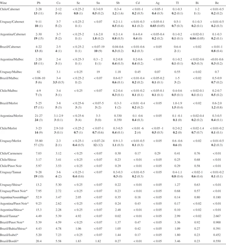
Table S1. Concentrations (in μg L-1) range, means (in bold) and standard deviations (in parenthesis) of minor and trace elements found in the wines.
Concentrations of K, P, Mg, Ca and Na are in mg L-1. Those wines marked with * only one sample was analysed
Wine K P Mg Ca Na Sr Fe Al Mn Rb
Chile/Cabernet 898-1230
1054 (161)
542-849
642 (133)
111-124
116 (53)
50-80
61 (12)
3-13
8 (4)
551-995
669 (185)
1770-4849
3373 (1547)
388-1676
1118 (468)
832-3270
1601 (979)
3377-4973
3969 (698)
Uruguay/Cabernet 502-852
618 (159)
525-597
578 (35)
79-85
83 (3)
40-67
51 (13)
17-40
24 (11)
520-847
724 (149)
907-1629
1261 (394)
230-394
327 (72)
1251-1867
1455 (282)
3108-3574
3246 (219)
Argentina/Cabernet 1184-1316
1244 (67)
534-895
665 (200)
92-108
101 (8)
48-71
60 (11)
20-55
39 (18)
697-991
844 (147)
1938-2271
2068 (178)
694-805
744 (56)
873-982
911 (62)
557-1247
905 (345)
Brazil/Cabernet 1068-1487
1222 (160)
350-552
476 (81)
84-98
90 (5)
62-84
74 (11)
14-69
34 (24)
365 -1382
771 (392)
454-1918
1254 (736)
296 -1130
572 (347)
1217-3232
2155 (747)
2348-7644
4804 (1977)
Argentina/Malbec 827 -1087
1013 (108)
627-900
713 (107)
100-116
107 (7)
57-79
66 (9)
10-63
32 (22)
705-1070
902 (151)
1387-2099
1824 (323)
486 -1208
703 (319)
798 -1125
1015 (133)
523-865
669 (139)
Uruguay/Malbec 908 554 85 62 55 842 3177 946 706 3072
Brazil/Malbec 938 -1187
1062 (176)
407 -572
489 (117)
87 -95
91 (4)
49 -51
50 (1)
56-62
59 (3)
593-1178
886 (414)
857-1015
936 (112)
530 -850
690 (226)
1761-1957
1859 (139)
5332-5391
5362 (42)
Chile/Malbec 1078-1117
1097 (27)
503-1358
930 (604)
105-113
109 (6)
28-49
38 (14)
3-16
10 (8)
760-846
803 (61)
2033-2078
2056 (32)
443 -653
548 (148)
2273-2545
2509 (192)
4264-4387
4326 (87)
Brazil/Merlot 1094-1300
1203 (104)
449-634
535 (93)
82-103
94 (11)
58-83
72 (13)
13-23 19 (5)
478-829
640 (177)
516-2098
1318 (791)
548 -1014
818 (242)
1784 -2407
2194 (355)
3253-6343
4970 (1573)
Argentina/Merlot 987 -1237
1112 (177)
329-661
495 (235)
97-110
104 (9)
65 -67 66 (1)
22-38
33 (6)
887-983
935 (68)
1227-1567
1397 (240)
555-695
625 (99)
641 -766
704 (88)
585-658
622 (52)
Chile/Merlot 955-1395
1094 (260)
559-997
718 (242)
99-117
108 (9)
51 -56 53 (2)
8-49
23 (22)
425-885
638 (232)
2231-2828
2524 (299)
765 -921
861 (84)
892 -975
938 (42)
1110- 3613
1986 (1410)
Uruguay/Merlot 895-1439
1167 (272)
545-595
567 (35)
84 -88 86 (2)
62 -75
68 (6)
19 -55
37 (18)
830-857
844 (14)
2400-2728
2564 (232)
801 -882
842 (41)
723 -1193
958 (235)
2729-3070
2900 (170)
Chile/Carmenere 1085 886 116 65 23 606 625 780 1096 5935
Chile/Shiraz 1340 302 116 73 10 1008 2327 182 840 2568
Chile/Pinot Noir 1048 217 106 68 9 580 3038 177 590 2237
Uruguay/Tannat 1126-1856
1417 (387)
564-612
582 (26)
79-81
80 (1)
73-107
88 (17)
17-67
40 (25)
897-1194
1070 (154)
398-3267
1511 (1539)
897-981
945 (43)
1043-1894
1351 (472)
2344-3813
Tabela S1. Continued
Wine K P Mg Ca Na Sr Fe Al Mn Rb
Uruguay/Shiraz* 195 595 87 102 14 1228 2827 871 1382 3965
Uruguay/Pinot Noir* 1255 597 80 78 46 948 785 1062 1119 2828
Argentina/Assemblage* 976 773 105 39 7 615 2285 613 984 1138
Argentina/Pinot Noir* 1541 538 98 98 23 892 908 673 1004 1235
Argentina/Shiraz* 1703 505 107 79 8 1400 2003 682 919 709
Brazil/Tannat* 1636 543 106 81 33 1014 1511 439 3295 5114
Brazil/Pinot Noir* 1222 544 901 59 12 585 1318 1030 1649 5215
Brazil/Bahia/Shiraz* 1350 509 89 71 8 637 2151 758 1052 2004
Brazil/Isabel* 893 368 90 75 2 559 1633 602 2434 4646
Brazil/Bordô* 890 390 100 978 4 507 1618 367 2273 3557
Wine Zn Ba Cu Ti V Li Mo Cr Ni As
Chile/Cabernet 214-926
592 (324)
133-195
155 (24)
64-177
113 (45)
101-171
136 (26)
21-137
65 (55)
7-14
11 (4)
2-91
31 (36)
2-22
13 (9)
3-16
12 (5)
4-23
12 (7)
Uruguay/Cabernet 337-818
526 (209)
142-184
168 (18)
124-247
170 (54)
75-182
141 (47)
19-88
54 (35)
19-30
25 (6)
3-5
4 (1)
17-25
20 (4)
27-43
34 (7)
3-21
11 (8)
Argentina/Cabernet 591 -685
630 (49)
122-410
229 (158)
20-249
149 (117)
132-158
149 (15)
21-67
43 (23)
175-283
226 (54)
5-19
12 (7)
15-31
25 (9)
15-42
28 (13)
11-15
13 (2)
Brazil/Cabernet 184-681
412 (189)
117-303
244 (73)
38-56
49 (7)
36-161
93 (50)
2-52
16 (21)
3-13
6 (4)
1-12
5 (4)
9-37
17 (12)
19-44
28 (10)
< 0.5-8
4 (3)
Argentina/Malbec 460-1239
800 (299)
100-158
134 (26)
23-133
107 (73)
111-168
145 (25)
< 0.9-80
34 (41)
71-354
173 (112)
1-10
6 (4)
6-37
23 (12)
20-38
29 (8)
4-28
14 (10)
Uruguay/Malbec 737 525 1290 179 42 21 5.5 17 33 8.5
Brazil/Malbec 308-530
419 (157)
432-481
457 (35)
28-161
95 (94)
79-112
96 (23)
3-5
4 (1)
3-5
4 (1)
1-4
3 (2)
20-43
31 (16)
11-18
15 (4)
1.7-2.0
1.8 (0.3)
Chile/Malbec 544-1181
863 (450)
452-513
483 (43)
73-77
75 (3)
124-179
152 (39)
29-83
56 (38)
5-11
8 (4)
3-23
13 (14)
24-32
28 (6)
3-28
16 (18)
5-16
11 (8)
Brazil/Merlot 232-891
619 (344)
279-675
425 (218)
39 -115
80 (38)
80-180
127 (57)
15-31
21 (9)
5-14
9 (5)
3-9
5 (3)
5-13
10 (4)
19-39
29 (10)
5-10
8 (3)
Argentina/Merlot 561-823
692 (185)
305-341
323 (25)
54-76
65 (15)
131-157
144 (18)
1-50
26 (51)
169-184 177 (11)
3-8
5 (3)
28-31 29 (1)
22-38
30 (11)
7-20
14 (7)
Chile/Merlot 670-1359
933 (372)
42-53
47 (5)
95-346
186 (130)
145-186
161 (22)
40-281
139 (126)
9-14
11 (3)
4-32
14 (16)
14-61
34 (24)
26-28
27 (1)
13 -79
35 (38)
Uruguay/Merlot 231-737
484 (253)
98-115
107 (8)
86-1210
648 (562)
121-144
133 (12)
64-70
68 (2)
21-49
35 (14)
4-6
5 (1)
5 -12
9 (4)
25-59
42 (17)
13 -14
13 (1)
Chile/Carmenere 923 105 290 165 35.1 3.19 5.41 55.1 23.9 10.1
Chile/Shiraz 174 108 123 153 42.5 4.31 4.67 12.4 24.3 11.2
Chile/Pinot Noir 186 121 98 70.2 44.3 3.92 6.84 10.6 14.7 13.9
Uruguay/Tannat 390-890
665 (254)
176-212
191 (19)
20.8-196
101 (88)
116-184
140 (38)
37-99
61 (33)
18-42
32 (10)
4-8
6 (2)
15-57
31 (23)
29-47
40 (8)
10-14
12 (2)
Uruguay/Shiraz* 358 162 182 157 34.8 20.9 4.20 21.2 48.4 13.8
Uruguay/Pinot Noir* 140 159 89 136 82.6 29.4 6.03 23.6 38.1 17.3
Argentina/Assemblage* 618 52.7 30.3 119 11.5 127 1.43 68.4 26.6 10.5
Argentina/Pinot Noir* 155 132 64 168 66.9 90.3 7.47 15.2 12.3 18.5
Argentina/Shiraz* 381 96 132 33 42.8 345 11.5 44.9 18.7 17.3
Brazil/Tannat* 444 293 76 144 62.9 27.3 13.8 37.1 40.9 15.1
Brazil/Pinot Noir* 499 91.1 124 156 76.5 9.85 11.4 50.2 42.0 15.8
Brazil/Bahia/Shiraz* 278 100 134 145 62.8 4.04 21.0 48.1 22.5 17.2
Brazil/Isabel* 767 479 118 118 74.0 3.75 9.53 26.5 11.5 15.6
Tabela S1. Continued
Wine Pb Co Se Sn Sb Cd Ag Tl Bi Be
Chile/Cabernet 2-28
13 (11)
2-12
5 (4)
< 0.25-2
0.8 (1)
0.3-0.9
0.5 (0.2)
0.3-4
1.2 (1.6)
< 0.01-1
0.2 (0.5)
< 0.05-1
0.4 (0.5)
0.1-0.3
0.2 (0.1)
1-2
1 (1)
< 0.01-0.5
0.2 (0.2)
Uruguay/Cabernet 9-11
10 (1)
3-7
5 (2)
< 0.25-2
1 (1)
< 0.07 0.2-1.1
0.5 (0.4)
< 0.01-0.3
0.1 (0.2)
< 0.05-0.1
0.03 (0.05)
0.5-1
0.7 (0.3)
0.1-0.3
0.2 (0.1)
< 0.01-0.5
0.2 (0.3)
Argentina/Cabernet 2-30
19 (15)
3-7
5 (2)
< 0.25-2
1 (1)
1.6-2.0
1.8 (0.2)
0.2-1.4
0.8 (0.5)
0.4-0.4
0.4 (0)
< 0.05-0.4
0.2 (0.2)
0.1-0.2
0.1 (0.1)
< 0.02-0.1
0.04 (0.05)
0.1-0.3
0.2 (0.1)
Brazil/Cabernet 4-22
13 (8)
2-5
4 (1)
< 0.25-2
1 (1)
< 0.07-19
10 (9)
0.04-0.6
0.3 (0.2)
< 0.01-0.6
0.2 (0.3)
< 0.05 0.6-4
2 (1)
< 0.02 < 0.01-1
0.8 (0.4)
Argentina/Malbec 2-20
15 (11)
2-4
3 (1)
< 0.25-3
1 (1)
0.3 – 2
1 (1)
0.2-0.8
0.4 (0.3)
0.2-0.6
0.4 (0.2)
< 0.05 0.1-0.2
0.1 (0.1)
< 0.02-0.6
0.3 (0.3)
<0.01-0.6
0.3 (0.2)
Uruguay/Malbec 82 3.1 < 0.25 19 1.18 0.45 0.07 0.55 < 0.02 0.7
Brazil/Malbec < 0.06-10
5 (6)
3-4
3.5 (0.5)
< 0.25-2
1 (2)
< 0.07 0.6-0.7
0.6 (0.1)
< 0.01-0.4
0.2 (0.2)
< 0.05-0.2
0.1 (0.1)
1-5
3 (2)
< 0.02 0.5-0.9
0.7 (0.2)
Chile/Malbec 4-9
7 (3)
3-4
3 (1)
< 0.25 < 0.07 0.2-0.4
0.3 (0.1)
< 0.01-0.2
0.1 (0.1)
< 0.05-0.1
0.1 (0.1)
0.4-0.6
0.5 (0.1)
< 0.02-0.1
0.1 (0.1)
0.2-0.7
0.5 (0.2)
Brazil/Merlot 5-25
17 (11)
3-8
5 (3)
< 0.25-6
3 (3)
< 0.07-5
3 (2)
0.3-3
1 (2)
< 0.01 -0.4
0.2 (0.2)
< 0.05 1.0-1.9
1.5 (0.4)
< 0.02 0.6-2.0
1.2 (0.8)
Argentina/Merlot 21-27
24 (3)
3.1-2.9
3 (0.1)
< 0.25-6
3 (4)
3-3
3 (0)
0.330 0.350
0.1 -0.6
0.4 (0.3)
< 0.05 0.1 -0.1
0.1 (0)
< 0.02-0.4
0.2 (0.2)
0.3-0.5
0.4 (0.1)
Chile/Merlot 3-23
14 (9)
2.9-3.0
3 (0.1)
< 0.25-2
0.7 (1)
< 0.07-1
0.7 (0.6)
0.3-0.5
0.4 (0.1)
< 0.01 -6
2 (4)
< 0.05 -1
0.5 (0.5)
0.2-0.2
0.2 (0)
< 0.02-1.4
0.7 (0.7)
< 0.01-0.2
0.1 (0.1)
Uruguay/Merlot 35-80
57 (23)
2-3
2 (1)
< 0.25-1
0.4 (0.5)
< 0.07-24
12 (12)
0.9-1.3
1.1 (0.3)
< 0.01-0.5
0.1 (0.3)
< 0.05 0.6 -0.6
0.6 (0)
< 0.02 < 0.01-0.5
0.2 (0.3)
Chile/Carmenere 7.03 3.12 < 0.25 < 0.07 0.30 0.17 0.29 0.41 0.76 < 0.01
Chile/Shiraz 3.17 3.41 < 0.25 < 0.07 0.23 < 0.01 < 0.05 0.25 0.68 < 0.01
Chile/Pinot Noir 5.97 3.53 < 0.25 < 0.07 0.29 < 0.01 < 0.05 0.29 0.58 < 0.01
Uruguay/Tannat 9-28
19 (10)
3-6
4 (2)
< 0.25-1
0.4 (0.6)
< 0.07 0.3-0.3
0.3 (0)
< 0.01-0.5
0.2 (0.3)
< 0.05 0.4-1.1
0.8 (0.4)
< 0.02-1
0.6 (0.4)
< 0.01-0.2
0.1 (0.1)
Uruguay/Shiraz* 13.2 5.30 < 0.25 < 0.07 0.22 < 0.01 < 0.05 1.27 0.63 < 0.01
Uruguay/Pinot Noir* 7.95 2.72 < 0.25 < 0.07 0.23 < 0.01 < 0.05 0.68 0.57 < 0.01
Argentina/Assemblage* 52.9 3.47 2.05 < 0.07 0.35 0.18 < 0.05 0.14 0.80 0.180
Argentina/Pinot Noir* 9.23 2.62 < 0.25 < 0.07 0.24 0.43 < 0.05 0.17 < 0.02 < 0.01
Argentina/Shiraz* 15.3 2.28 < 0.25 < 0.07 2.48 < 0.01 < 0.05 0.10 < 0.02 < 0.01
Brazil/Tannat* 4.49 5.39 4.92 < 0.07 0.02 < 0.01 < 0.05 2.99 < 0.02 2.667
Brazil/Pinot Noir* 5.39 4.59 < 0.25 < 0.07 1.37 0.47 < 0.05 3.36 0.92 0.900
Brazil/Bahia/Shiraz* 4.43 4.78 1.06 < 0.07 1.05 0.42 < 0.05 1.09 0.27 0.391
Brazil/Isabel* 5.20 7.23 < 0.25 < 0.07 1.44 0.17 < 0.05 1.80 0.23 0.452
Tabela S1. Continued
Wine U La Ce Pr Nd Sm Eu Gd Tb
Chile/Cabernet < 0.02-0.4
0.2 (0.1)
0.2-3
1 (1)
0.5-2.5
1 (1)
< 0.02-0.2
0.1 (0.1)
< 0.02-1
0.3 (0.4)
< 0.02-0.09
0.05 (0.04)
< 0.01-0.1
0.03 (0.04)
< 0.01-0.1
0.08 (0.04)
< 0.002-0.01
0.01 (0.01)
Uruguay/Cabernet 0.2-0.5
0.3 (0.1)
< 0.02-0.5
0.1 (0.2)
0.3-0.7
0.5 (0.2)
< 0.02 -0.1
0.08 (0.02)
< 0.02 < 0.02-0.1
0.03 (0.06)
< 0.01-0.05
0.02 (0.03)
0.06-0.1
0.07 (0.03)
< 0.002-0.01
0.04 (0.07)
Argentina/Cabernet 0.2-2
1.4 (1.1)
0.4-1
0.7 (0.3)
0.8-1
0.9 (0.1)
0.1-0.3
0.2 (0.1)
0.1-0.5
0.3 (0.2)
0.05-0.09
0.07 (0.02)
< 0.008 0.07-0.2
0.1 (0.1)
< 0.002
Brazil/Cabernet < 0.02-0.5
0.1 (0.2)
< 0.02 -1
0.6 (0.5)
0.5-2
1 (0.5)
< 0.02-0.2
0.1 (0.1)
< 0.02 < 0.02-0.2
0.1 (0.1)
< 0.01-0.06
0.03 (0.03)
0.06-0.2
0.15 (0.05)
< 0.002-0.02
0.01 (0.01)
Argentina/Malbec 0.2-2.2
1.1 (0.7)
0.4-1.6
0.9 (0.5)
0.4-1
0.6 (0.3)
< 0.02-0.1
0.07 (0.02)
< 0.02-0.3
0.1 (0.1)
0.05-0.09
0.07 (0.02)
< 0.01 < 0.01-0.08
0.06 (0.02)
< 0.002
Uruguay/Malbec 1.2 0.3 0.5 0.06 < 0.02 0.050 < 0.01 0.05 < 0.002
Brazil/Malbec < 0.02-0.2
0.1 (0.1)
0.4-1.7
1.0 (0.7)
0.4-0.4
0.4 (0)
< 0.02-0.06
0.05 (0.01)
< 0.02 < 0.02-0.04
0.02 (0.02)
< 0.01 < 0.01 -0.04
0.02 (0.02)
< 0.002
Chile/Malbec 0.4-0.6
0.5 (0.1)
0.2-0.6
0.4 (0.2)
0.3-0.9
0.6 (0.3)
< 0.02-0.1
0.1 (0.1)
< 0.02 < 0.02-0.07
0.04 (0.03)
< 0.01 < 0.01-0.07
0.04 (0.03)
< 0.002 0.012
Brazil/Merlot < 0.02-0.3
0.2 (0.1)
0.5-0.7
0.6 (0.1)
0.9-1.4
1.1 (0.3)
< 0.02-0.2
0.1 (0.1)
< 0.02-0.6
0.3 (0.3)
< 0.02-0.1
0.1 (0.01)
< 0.01 0.06-0.1
0.1 (0.04)
< 0.002-0.02
0.01 (0.01)
Argentina/Merlot 1.0-1.5
1.3 (0.3)
0.3-0.4
0.3 (0.1)
0.5-0.6
0.5 (0.1)
< 0.02 0.2-0.2
0.2 (0)
0.03-0.04
0.03 (0.01)
< 0.01 0.04-0.05
0.04 (0.01)
< 0.002
Chile/Merlot 0.3-1.2
0.6 (0.5)
0.3-2.8
1.2 (1.4)
0.3-3.3
1.4 (1.6)
< 0.02-1.5
0.6 (0.8)
< 0.02-1
0.4 (0.5)
< 0.02 -1
0.4 (0.6)
< 0.01 -0.6
0.2 (0.4)
0.05 -0.2
0.1 (0.1)
< 0.002
Uruguay/Merlot 0.3 -1.1
0.7 (0.6)
0.3-0.3
0.3 (0)
0.4-0.5
0.4 (0.1)
< 0.02-0.07
0.3 (0.4)
< 0.02-0.2
0.1 (0.1)
< 0.02-0.05
0.02 (0.03)
< 0.01 0.06-0.06
0.06 (0)
< 0.002
Chile/Carmenere 0.15 <0.02 0.30 < 0.02 < 0.001 < 0.02 < 0.008 < 0.01 < 0.002
Chile/Shiraz 0.27 0.30 0.32 < 0.02 < 0.02 0.07 0.01 0.06 < 0.002
Chile/Pinot Noir < 0.02 0.83 0.62 < 0.02 < 0.02 0.07 0.02 0.06 < 0.002
Uruguay/Tannat 0.4-0.8
0.6 (0.2)
0.2-0.4
0.3 (0.1)
0.2-0.8
0.5 (0.3)
< 0.02-0.1
0.05 (0.03)
< 0.02-0.4
0.2 (0.2)
0.07-0.09
0.08 (0.01)
< 0.01 0.06-0.08
0.07 (0.01)
< 0.002
Uruguay/Shiraz* 0.97 0.88 0.35 < 0.02 < 0.02 0.07 0.02 0.06 < 0.002
Uruguay/Pinot Noir* 1.31 0.80 0.67 < 0.02 < 0.02 0.07 0.02 0.06 < 0.002
Argentina/Assemblage* 2.09 0.26 0.33 0.05 0.22 0.07 < 0.01 < 0.01 < 0.002
Argentina/Pinot Noir* 1.04 0.23 0.56 < 0.02 < 0.02 0.17 0.02 0.16 < 0.002
Argentina/Shiraz* < 0.02 0.63 0.87 0.10 0.37 0.07 0.02 0.06 < 0.002
Brazil/Tannat* < 0.02 1.61 1.91 0.61 < 0.02 0.07 0.02 0.06 < 0.002
Brazil/Pinot Noir* 0.33 0.80 1.68 0.22 < 0.02 0.17 0.05 0.16 < 0.002
Brazil/Bahia/Shiraz* 0.18 1.47 3.02 0.39 1.44 0.23 0.06 0.19 < 0.002
Brazil/Isabel* 0.18 0.64 0.950 0.11 0.34 0.09 0.05 0.07 0.01
Tabela S1. Continued
Wine Dy Ho Er Tm Yb Lu
Chile/Cabernet < 0.01-0.03
0.01 (0.02)
< 0.002 < 0.002-0.06
0.02 (0.04)
< 0.002 < 0.005 < 0.002-0.02
0.01 (0.01)
Uruguay/Cabernet < 0.01-0.08
0.04 (0.03)
< 0.002 < 0.002-0.02
0.01 (0.01)
< 0.002 < 0.005 < 0.002
Argentina/Cabernet 0.06-0.08
0.07 (0.01)
< 0.002-0.02
0.01 (0.01)
0.04-0.05
0.04 (0.01)
< 0.002 < 0.005-0.04
0.01 (0.03)
< 0.002
Brazil/Cabernet < 0.01-0.1
0.09 (0.06)
< 0.002-0.05
0.02 (0.02)
< 0.002-0.1
0.07 (0.05)
< 0.002-0.02
0.01 (0.01)
< 0.005-0.1
0.05 (0.06)
< 0.002-0.02
0.01 (0.01)
Argentina/Malbec 0.03-0.08
0.06 (0.02)
< 0.002-0.01
0.01 (0.01)
< 0.002-0.05
0.03 (0.02)
< 0.002-0.01
0.01 (0.01)
< 0.005 < 0.002-0.01
0.01 (0.01)
Uruguay/Malbec 0.05 0.01 0.04 < 0.002 < 0.005 < 0.002
Brazil/Malbec < 0.01-0.03
0.01 (0.02)
< 0.002 < 0.002-0.03
0.01 (0.02)
< 0.002 < 0.005 < 0.002
Chile/Malbec < 0.01-0.07
0.04 (0.03)
< 0.002 0.01-0.05
0.03 (0.02)
< 0.002 < 0.005 < 0.002-0.01
0.01 (0.01)
Brazil/Merlot < 0.01-0.1
0.08 (0.02)
< 0.002-0.03
0.01 (0.02)
< 0.002-0.07
0.05 (0.03)
< 0.002-0.01
0.01 (0.01)
< 0.005-0.08
0.03 (0.04)
< 0.002-0.01
0.01 (0.01)
Argentina/Merlot 0.04-0.04
0.04 (0)
< 0.002-0.01
0.01 (0.01)
0.03 -0.03
0.03 (0)
< 0.002 0.03-0.04
0.03 (0.01)
< 0.002-0.01
0.01 (0.01)
Chile/Merlot < 0.01-0.2
0.1 (0.1)
< 0.002 < 0.002-0.1
0.05 (0.05)
< 0.002-0.01
0.01 (0.01)
< 0.005 < 0.002-0.02
0.01 (0.01)
Uruguay/Merlot < 0.01-0.06
0.04 (0.02)
< 0.002-0.01
0.01 (0.01)
0.02-0.04
0.03 (0.01)
< 0.002 < 0.005-0.04
0.02 (0.02)
< 0.002
Chile/Carmenere 0.026 < 0.002 0.02 0.01 < 0.005 < 0.002
Chile/Shiraz < 0.01 < 0.002 < 0.002 < 0.002 < 0.005 < 0.002
Chile/Pinot Noir < 0.01 < 0.002 < 0.002 < 0.002 < 0.005 < 0.002
Uruguay/Tannat < 0.01-0.1
0.04 (0.06)
< 0.002 < 0.002 0.010 < 0.005 < 0.002-0.01
0.01 (0.01)
Uruguay/Shiraz* < 0.01 < 0.002 < 0.002 < 0.002 < 0.005 < 0.002
Uruguay/Pinot Noir* < 0.01 < 0.002 < 0.002 < 0.002 < 0.005 < 0.002
Argentina/Assemblage* 0.04 < 0.002 < 0.002 < 0.002 < 0.005 0.01
Argentina/Pinot Noir* 0.13 0.03 0.06 0.01 < 0.005 0.0182
Argentina/Shiraz* < 0.01 < 0.002 < 0.002 < 0.002 < 0.005 < 0.002
Brazil/Tannat* < 0.01 < 0.002 < 0.002 < 0.002 < 0.005 < 0.002
Brazil/Pinot Noir* 0.13 0.03 0.06 0.01 < 0.005 0.02
Brazil/Bahia/Shiraz* 0.20 < 0.002 0.12 0.02 < 0.005 0.03
Brazil/Isabel* 0.17 < 0.002 0.04 0.01 < 0.005 0.01