Probabilist Set Inversion using Pseudo-Intervals Arithmetic
A. KENOUFI
Received on November 10, 2012 / Accepted on January 28, 2014
ABSTRACT.In this paper, one presents how to use a new interval arithmetic framework based on free algebra construction, called pseudo-intervals, which is associative and distributive and permits to build well-defined inclusion function for interval semi-group and for its associated vector space. One introduces theψ-algorithm (Probabilist Set Inversion), which performs set inversion of functions and exhibits some numerical examples.
Keywords:Free algebra, pseudo-interval and interval arithmetic, set inversion, probability.
1 SET INVERSION
One of the most recurrent problem arising in sciences and engineering is to perform adjustments of a system in order to get the desired performances. For example, how to set-up a car engine so that some polluting gases ratio are less than a certain amount, or how to settle a robot to make it moving toward a desired target. Such kind of problem are dealing with the inversion of the relation between adjustments and desired performances.
Let us noteR⊂Rnthe set of feasible adjustments, andP⊂Rpthe set of desired performance
of a system. The mathematical modelling of the problem consists of the computation ofS = f−1(P)∩R, as shown on Figure (1), where f :Rn →Rpis the function giving performances
from adjustments. Since real number sets can be written as union of intervals, one has to perform this set inversion within the interval semi-groupIR[1]. Some powerful set inversion methods are
have been developed those last years, such asSIvIA[18] (Set InversionviaInterval Arithmetic) which is based on interval arithmetic [2, 6, 7, 8, 9, 10, 11, 12, 32, 33, 34, 35, 36].
The first mathematician who has used intervals was the famous Archimedes from Syracuse (287-212 b.C). He has proposed a two-sides bounding ofπ: 3+1071 < π <3+17using polygons and a systematic method to improve it. In the beginning of the twentieth century, the mathematician and physicist Wiener, published two papers [3, 4], and used intervals to give an interpretation to the position and the time of a system. More papers on the subject were written [5, 6, 7, 36]
Figure 1: R⊂ Rnis the set of feasible adjustments, andP ⊂ Rpthe set of desired performance of a system. Set inversion computesS= f−1(P)∩R.
only after Second World War. Nowadays, we consider R.E. Moore [8, 9, 10, 11, 12] as the first mathematician who has proposed a framework for interval arithmetic and analysis. The interval arithmetic, or interval analysis has been introduced to compute very quickly range bounds (for example if a data is given up to an incertitude). Now interval arithmetic is a computing system which permits to perform error analysis by computing mathematics bounds. The extensions of the areas of applications are important: non linear problems, PDE, inverse problems. It finds a large place of applications in controllability, automatism, robotics, embedded systems, biomedi-cal, haptic interfaces, form optimization, analysis of architecture plans, ...
Interval calculations are used nowadays as a powerful tool for global optimization and set in-version [8, 9, 10, 11, 13, 18, 36]. Several groups have developed some software and libraries to perform those new approaches such asINTLAB[19],INTOPT90andGLOBSOL[20], Numer-ica [21]. But their Achille’s heel is the construction of the inclusion function from the natural one due to the lack of distributivity. Some approaches have developed methods to circumvent it with using boolean inclusion tests, series or limited expansions of the natural function where the derivatives are computed at a certain point of the intervals. Nevertheless, those transfers from real functions to functions defined on intervals are not systematic and not given by a formal process. This yields to the fact that the inclusion function definition has to be adapted to each problem with the risk to miss the primitive scope. Moreover, differential calculus and linear algebra need to be performed in the framework of vector space theory and not within semi-group one.
This article reminds first the definition and characteristics of the intervals semi-groupIRand
the construction of its associated vector spaceIR. After that it is explained how to get an
asso-ciative and distributive arithmetic of intervals, called pseudo-intervals arithmetic, by embedding the vector space into afree algebra[2]. After that, one proposes a clear and simple scheme to build inclusion functions from the natural one for the semi-group and the vector space.
2 AN ALGEBRAIC APPROACH FOR INTERVALS
An intervalX is defined as a non-empty, closed and connected set of real numbers. One writes real numbers as intervals with same bounds,∀a ∈ R,a ≡ [a,a]. We denote by IR = P1
the set of intervals ofR. The arithmetic operations on intervals, calledMinkowski or classical operations, are defined such that the result of the corresponding operation on elements belong-ing to operand intervals belongs to the resultbelong-ing interval. That is, if⋄denotes one of the usual operations+,−,∗, /, we have, ifX and Y are closed intervals ofR,
X⋄Y = {x⋄y/x∈ X, y∈Y}, (2.1)
Although,IRis provided with a pseudo-inverse operation, it does not satisfyX−X =0, and hence a subtraction in the usual sense cannot be obtained. In many problems using interval arith-metic, that is the setIRwith the Minkowski operations, there exists an informal transfers
prin-ciple which permits, to associate with a real function f a function define on the set of intervals
IRwhich coincides with f on the interval reduced to a point. But this transferred function is not unique. For example, if we consider the real function f(x)=x2+x =x(x+1), we associate naturally the functions f1, f2 :IR−→IRgiven by f1(X)=X(X+1)and f2(X)=X2+X.
These two functions do not coincide. Usually this problem is removed considering the most interesting transfers. But the qualitative “interesting” depends of the studied model and it is not given by a formal process.
In this section, we determine a natural extensionIRofIRprovided with a vector space
struc-ture. The vectorial subtractionXY does not correspond to the semantic difference of intervals and the intervalX has no real interpretation. But these “negative” intervals have a computa-tional role.
An algebraic extension of the classical interval arithmetic, called generalized interval arith-metic [13, 36] has been proposed first by M. Warmus [6, 7]. It has been followed in the seventies by H.-J. Ortolf & E. Kaucher [37, 42, 43, 44, 45]. In this former interval arithmetic, the intervals form a group with respect to addition and a complete lattice with respect to inclusion. In order to adapt it to semantic problems, Gardenes et al. have developed an approach called modal in-terval arithmetic [46, 47, 48, 49, 50, 51]. S. Markov and others investigate the relation between generalized intervals operations and Minkowski operations for classic intervals and propose the so-called directed interval arithmetic, in which Kaucher’s generalized intervals can be viewed as classic intervals plus direction, hence the name directed interval arithmetic [32, 33]. In this arithmetic framework, proper and improper intervals are considered as intervals with sign [34]. Interesting relations and developments for proper and improper intervals arithmetic and for ap-plications can be found in literature [38, 39, 40].
Our approach [2], that we remind below in this article, is similar to the previous ones in the sense that intervals are extended to generalized intervals; intervals and anti-intervals correspond respectively to the proper and improper ones. However we use a construction which is more canonical and based on the semi-group completion into a group, which permits then to build the associated real vector space, and to get an analogy with directed intervals.
2.1 Interval semi-group
LetIRbe the set of intervals. It is in one to one correspondence and can be represented as a
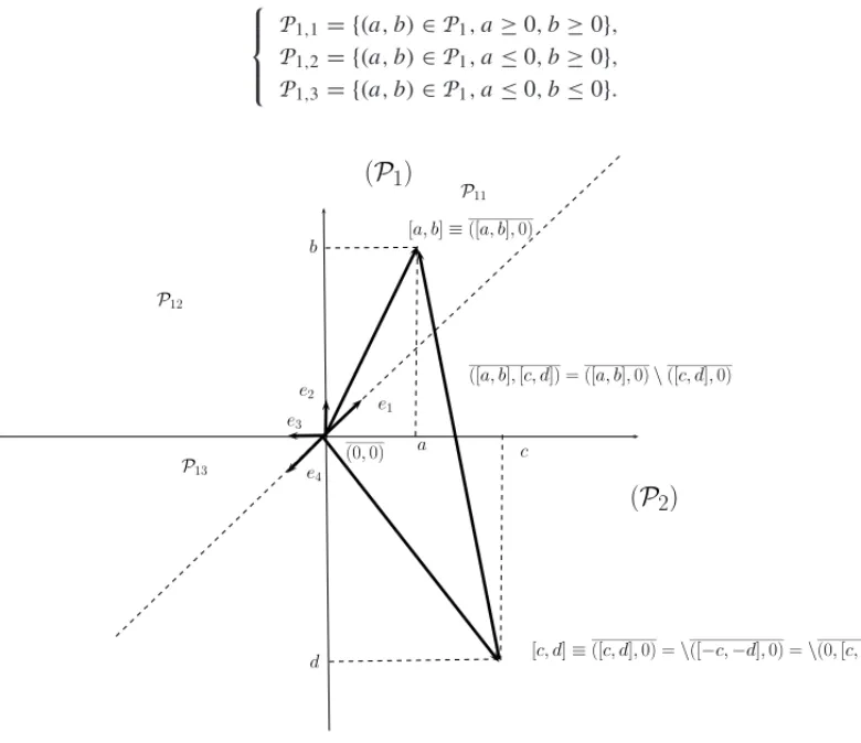
point in the half-plane ofR2,P1 = {(a,b)∈ R2,a ≤ b}. The setP2 = {(a,b)∈R2,a ≥b}
is the set of anti-intervals.IRis closed for the addition and endowed with a regular semi-group
structure. The subtraction onIR, which is not the symmetric operation of+, corresponds to the
following operation onP1:
(a,b)−(c,d)=(a,b)+s◦s0(c,d),
wheres0is the symmetry with respect to 0, andswith respect to. The multiplication∗is not globally defined. Consider the following subset ofP1:
⎧ ⎪ ⎨ ⎪ ⎩
P1,1= {(a,b)∈P1,a≥0,b≥0},
P1,2= {(a,b)∈P1,a≤0,b≥0},
P1,3= {(a,b)∈P1,a≤0,b≤0}.
a
b [a, b]≡([a, b],0)
P11
P12
P13
(
P
1)
(
P
2)
e1
e2
e3
e4
(0,0)
([a, b],[c, d]) = ([a, b],0)\([c, d],0)
[c, d]≡([c, d],0) =\([−c,−d],0) =\(0,[c, d])
c
d
Figure 2:Representation of intervals in the half plane ofR2.
We have the following cases:
1. If (a,b), (c,d) ∈ P1,1 the product is written(a,b)∗(c,d) = (ac,bd). The vectors
e1=(1,1)ande2=(0,1)generateP1,1that is any(x,y)inP1,1, can be decomposed as
The multiplication corresponds in this case to the following associative commutative
algebra:
e1e1=e1,
e1e2=e2e1=e2e2=e2.
2. Assume that (a,b) ∈ P1,1 and (c,d) ∈ P1,2 so c ≤ 0 and d ≥ 0. Thus we obtain
(a,b)∗(c,d)=(bc,bd)and this product does not depend ofa. Then we obtain the same result for anya <b. The product(a,b)∗(c,d)=(bc,bd)corresponds to
e1e1=e2e1=e1
e1e2=e2e2=e2
This algebra is not commutative and it is different from the previous.
3. If(a,b) ∈ P1,1and(c,d) ∈ P1,3 thena ≥ 0,b ≥ 0 andc ≤ 0,d ≤ 0 and we have
(a,b)∗(c,d)= (bc,ad). Lete1 =(1,1),e2 =(0,1). This product corresponds to the
following associative algebra:
⎧ ⎪ ⎨ ⎪ ⎩
e1e1=e1,
e1e2=e2,
e2e1=e1−e2.
This algebra is not associative because(e2e1)e1 = e2(e1e1). We have similar results for
the cases(P1,2,P1,2), (P1,2,P1,3)and(P1,3,P1,3).
An objective of this paper is to present an associative algebra which contains all these results.
2.2 The real vector spaceIR
We recall briefly the construction proposed by Markov [14] to define a structure of abelian group. As(IR,+)is a commutative and regular semi-group, the quotient set, denoted by IR,
associated with the equivalence relations:
(A,B)∼(C,D)⇐⇒A+D=B+C,
for allA,B,C,D ∈IR, is provided with a structure of abelian group for the natural addition:
(A,B)+(C,D)=(A+C,B+D)
where(A,B)is the equivalence class of(A,B). We denote by(A,B)the inverse of(A,B) for the interval addition.
Naturally, the group IR is isomorphic to the additive group R2 by the isomorphism
(([a,b],[c,d])→ (a −c,b−d)(Fig. 2). We find the notion of generalized interval and this yields immediately to the resulting result:
Proposition 1.LetX=(X,Y)be inIR. Thus
(1) If l(Y) <l(X), there is an unique A∈IR Rsuch thatX=(A,0),
(2) If l(Y) >l(X), there is an unique A∈IR Rsuch thatX=(0,A)=(A,0),
(3) If l(Y)=l(X), there is an unique A=α∈Rsuch thatX=(α,0)=(0,−α).
Any elementX =(A,0)withA ∈IR−Ris said positive and we writeX>0. Any element X = (0,A) with A ∈ IR−R is said negative and we writeX < 0. We write X ≥ X′ if XX′≥0. For example ifXandX′are positive,X ≥X′⇐⇒l(X)≥l(X′). The elements (α,0)withα∈R∗are neither positive nor negative.
In [14], one defines on the abelian groupIR, a structure of quasi linear space. Our approach is a
little bit different. We propose to construct a real vector space structure. We consider the external multiplication:
· :R×IR−→IR
defined, for allA∈IR, by
α·(A,0) =(αA,0), α·(0,A) =(0, αA),
for allα >0. Ifα <0 we putβ = −α. So we put:
α·(A,0) =(0, βA), α·(0,A) =(βA,0).
We denoteαXinstead ofα·X. This operation satisfies
1. For anyα∈RandX∈IRwe have:
α(X)=(αX), (−α)X =(αX).
2. For allα, β∈R, and for allX,X′∈IR, we have ⎧
⎪ ⎨ ⎪ ⎩
(α+β)X=αX+βX, α(X+X′)=αX+αX′, (αβ)X=α(βX).
Theorem 1. The triplet (IR,+,·)is a real vector space and the vectors X1 = ([0,1],0)
Proof. We have the following decompositions:
([a,b],0) =(b−a)X1+aX2,
(0,[c,d]) =(c−d)X1−cX2.
The linear map
ϕ :IR−→R2
defined by
ϕ( ([a,b],0) )=(b−a,a), ϕ( (0,[c,d]) )=(c−d,−c)
is a linear isomorphism andIRis canonically isomorphic toR2. The following map
||.|| :IR −→ R+ (2.2)
(X,0) → l(X)+ |c(X)| (2.3)
or (2.4)
(0,X) → l(X)+ |c(X)| (2.5)
with respectivelyl(X)andc(X)the width and the center of the intervalX, is obviously a norm. SinceIRis isomorphic toR2which is complete, this yields to the fact that this norm endowsIR
with a Banach space structure. Thus, it is possible to perform differential calculus inIR[22].
3 A 4-dimensional free algebra associated withIR
We define in this section a four-dimensional associative and distributivefree algebrain which the real vector space is embedded.
3.1 Definition ofA4
In introduction, we have observed that the semi-groupIRis identified toP1,1∪P1,2∪P1,3. Let
us consider the following vectors ofR2: ⎧ ⎪ ⎪ ⎪ ⎨ ⎪ ⎪ ⎪ ⎩
e1=(1,1),
e2=(0,1),
e3=(−1,0),
e4=(−1,−1).
They correspond to the intervals[1,1],[0,1],[−1,0], and[−1,−1]. Any point ofP1,1∪P1,2∪
P1,3admits the decomposition
(a,b)=α1e1+α2e2+α3e3+α4e4
withαi ≥0. The dependence relations between the vectorsei are
e2=e3+e1
Thus there exists a unique decomposition of(a,b)in a chosen basis such that the coefficients are non negative. These basis are{e1,e2}forP1,1,{e2,e3}forP1,2,{e3,e4}forP1,3. Let us consider
the free algebra of basis{e1,e2,e3,e4}whose products correspond to the Minkowski products.
The multiplication table is
e1 e2 e3 e4
e1 e1 e2 e3 e4
e2 e2 e2 e3 e3
e3 e3 e3 e2 e2
e4 e4 e3 e2 e1
This algebra is associative and its elements are called pseudo-intervals.
3.2 Pseudo-intervals product
Letϕ : IR → A4 the natural injective embedding,ψ the canonical embedding fromA4 to
A4/Fandϕ′=ψ◦ϕ. If we identify an interval with its image inA4, one has:
The applicationϕis not bijective. Its image on the elementsX=(X,0)=([a,b],0)is:
⎧ ⎪ ⎨ ⎪ ⎩
X= [a,b] ∈P1,1, ϕ(X)=ae1+(b−a)e2 (a ≥0,b−a ≥0)
X= [a,b] ∈P1,2, ϕ(X)= −ae3+be2 (−a≥0,b≥0)
X= [a,b] ∈P1,3, ϕ(X)= −be4+(b−a)e3 (−b≥0,b−a≥0).
Consider inA4the linear subspaceFgenerated by the vectorse1−e2+e3,e1+e4. As
(e1+e4)(e1+e4)=2(e1+e4)
(e1+e4)(e1−e2+e3)=e1+e4
(e1−e2+e3)(e1−e2+e3)=e1,
F is not a sub-algebra ofA4. Let us consider the map
ϕ:IR→A4/F
defined fromϕand the canonical projection on the quotient vector spaceA4/F. A vectorX =
αiei ∈A4is equivalent to a vector ofA4with positive components if and only if
α2+α3≥0.
In this case, all the vectors equivalent tox=αiei withα2+α3≥0 correspond to the interval
[α1−α3−α4, α1+α2−α4]ofIR. Thus we have for any equivalent classes ofA4/Fassociated
withαiei withα2+α3≥0 a pre-image inIR. The mapϕis injective. In fact, two intervals
belonging to pieces P1,i,P1,j withi = j, have distinguish images. Now if (a,b)and(c,d)
belong to the same piece, for exampleP1,1, thus
Ifϕ(c,d)=ϕ(a,b), there areλ, µ∈Rsuch that(c,d)=(a+λ+µ,b−a−λ, λ, µ). This givesa =c,b =d. We have the same results for all the other pieces. Thusϕ :IR→A4/Fis
bijective on its image, that is the hyperplane ofA4/Fcorresponding toα2+α3≥0.
Practically the multiplication of two intervals will so be made: let X,Y ∈ R. Thus X =
αiei,Y =βiei withαi, βj ≥0 and we have the product
X•Y =ϕ−1(ϕ′(X).ϕ′(Y))
this product is well defined becauseϕ′(X).ϕ′(Y)∈ I mϕ. This product is distributive because
X•(Y +Z) =ϕ−1(ϕ′(X).ϕ′(Y +Z)) =ϕ−1(ϕ′(X).(ϕ′(Y)+ϕ′(Z)) =ϕ−1(ϕ′(X).ϕ′(Y)+ϕ′(X).ϕ′(Z)) =X•Y +X•Z
Remark. We have
ϕ−1(ϕ′(X).ϕ′(Y +Z))=ϕ−1(ϕ′(X)).ϕ−1(ϕ′(Y +Z))).
We shall be careful not to return inIRduring the calculations as long as the result is not found.
Otherwise we find the semantic problems of the distributivity.
We extend naturally the mapϕ:IR→A4toIRby
ϕ(A,0)=ϕ(A) ϕ(0,A)= −ϕ(A)
for everyA∈IR.
Theorem 2.The multiplication
X•Y=ϕ−1(ϕ′(X).ϕ′(Y))
is distributive with respect the addition.
Proof. This is a direct consequence of the previous computations.
3.3 Pseudo-intervals division
Division between intervals can also be defined with solvingX ·Y = (1,0,0,0)inA4or in a
isomorphic algebra. InA4we consider the change of basis ⎧
⎪ ⎨ ⎪ ⎩
e1′ =e1−e2
ei′ =ei,i =2,3
This change of basis shows thatA4is isomorphic toA′4
e′1 e′2 e′3 e4′ e′1 e′1 0 0 e4′ e′2 0 e′2 e′3 0 e′3 0 e′3 e′2 0
e′4 e′4 0 0 e1′ .
The unit ofA′4is the vectore′1+e2′. This algebra is a direct sum of two ideals:A′4 = I1+I2
whereI1is generated bye′1ande′4andI2is generated bye′2ande′3. It is not an integral domain,
that is, we have divisors of 0. For examplee′1·e2′ =0.
Proposition 2. The multiplicative groupA∗4of invertible elements ofA4is the set of elements
x=(x1,x2,x3,x4)such that
x4= ±x1,
x3= ±x2.
This means that the invertible intervals do not contain 0. If x ∈A∗4we have:
x−1= x1 x12−x42,
x2
x22−x32, x3
x22−x32, x4
x12−x42
.
3.4 Monotony property
Let us compute the product of intervals using the product in A4 and compare it with the
Minkowski product. LetX = [a,b]andY = [c,d]two intervals.
Lemma 1.If X and Y are not in the same pieceP1,i, then X •Y corresponds to the Minkowski
product.
Proof. i) IfX ∈ P1,1andY ∈ P1,2 thenϕ(X) =(a,b−a,0,0)andϕ(Y) =(0,d,−c,0).
Thus
ϕ(X)ϕ(Y) =(ae1+(b−a)e2)(de2−ce3)
=bde2−cbe3
=(0,bd,−cb,0) =ϕ([cb,bd]).
ii) IfX ∈P1,1andY ∈P1,3thenϕ(X)=(a,b−a,0,0)andϕ(Y)=(0,0,d−c,−d). Thus
ϕ(X)ϕ(Y) =(ae1+(b−a)e2)((d−c)e3−de4)
=(ad−bc)e3−ade4
iii) IfX ∈P1,2andY ∈P1,3thenϕ(X)=(0,b,−a,0)andϕ(Y)=(0,0,d−c,−d). Thus
ϕ(X)ϕ(Y) =(be2−ae3)((d−c)e3−de4)
=ace2−bce3
=(0,ac,−cb,0) =ϕ([bc,ad]).
Lemma 2.If X an Y are both in the same pieceP1,1orP1,3, then the product X•Y corresponds
to the Minkowski product. The proof is analogous to the previous.
Let us assume thatX = [a,b]andY = [c,d]belong toP1,2. Thusϕ(X)=(0,b,−a,0)and
ϕ(Y)=(0,d,−c,0). We obtain
X Y =(be2−ae3)(de2−ce3)=(bd+ac)e2+(−bc−ad)e3.
Thus
[a,b][c,d] = [bc+ad,bd+ac].
This result is greater that all the possible results associated with the Minkowski product. How-ever, we have the following property:
Proposition 3.Monotony property:LetX1,X2∈IR. Then
X1⊂X2=⇒X1•Z⊂X2•Zfor allZ∈IR.
ϕ(X1)≤ϕ(X2)=⇒ϕ(X1•Z)≤ϕ(X2•Z)
The order relation onA4that ones uses here is ⎧
⎪ ⎪ ⎪ ⎪ ⎪ ⎨ ⎪ ⎪ ⎪ ⎪ ⎪ ⎩
(x1,x2,0,0)≤(y1,y2,0,0)⇐⇒y1≤x1andx2≤y2,
(x1,x2,0,0)≤(0,y2,y3,0)⇐⇒ x2≤ y2,
(0,x2,x3,0)≤(0,y2,y3,0)⇐⇒x3≤ y3andx2≤y2,
(0,0,x3,x4)≤(0,y2,y3,0)⇐⇒ x3≤ y3,
(0,0,x3,x4)≤(0,0,y3,y4)⇐⇒x3≤ y3andy4≤x4.
Proof. Let us note that the second property is equivalent to the first. It is its translation in A4. We can suppose thatX1 andX2 are intervals belonging moreover to P1,2: ϕ(X1) =
(0,b,−a,0), ϕ(X2)=(0,d,−c,0). Ifϕ(Z)=(z1,z2,z3,z4), then
ϕ(X1•Z)=(0,bz1+bz2−az3−az4,−az1+bz3−az2+bz4,0),
ϕ(X2•Z)=(0,d z1+d z2−cz3−cz4,−cz1+d z3−cz2+d z4,0).
Thus
ϕ(X1•Z)≤ϕ(X2•Z)⇐⇒
(b−d)(z1+z2)−(a−c)(z3−z4)≤0,
−(a−c)(z1+z2)+(b−d)(z3=z4)≤0.
4 THE ALGEBRASAnAND AN BETTER RESULT OF THE PRODUCT
We can refine our result of the product to come closer to the result of Minkowski. Consider the one dimensional extensionA4⊕Re5=A5, wheree5is a vector corresponding to the interval
[−1,1]ofP1,2. The multiplication table ofA5is
e1 e2 e3 e4 e5
e1 e1 e2 e3 e4 e5
e2 e2 e2 e3 e3 e5
e3 e3 e3 e2 e2 e5
e4 e4 e3 e2 e1 e5
e5 e5 e5 e5 e5 e5
The pieceP1,2is writtenP1,2=P1,2,1∪P1,2,1whereP1,2,1= {[a,b],−a ≤b}andP1,2,2 =
{[a,b],−a≥b}. If X= [a,b] ∈P1,2,1andY = [c,d] ∈P1,2,2, thus
ϕ(X).ϕ(Y)=(0,b+a,0,0,−a).(0,0,−c−d,0,d)=(0,−(a+b)(c+d),0,0,a(c+d)+bd).
Thus we have
X•Y = [−bd−ac−ad,−bc].
Example. Let X = [−2,3]andY = [−4,2]. We have X ∈ P1,2,1 andY ∈ P1,2,2. The
product inA4gives
X•Y = [−16,14].
The product inA5gives
X•Y = [−12,10].
The Minkowski product is
[−2,3].[−4,2] = [−12,8].
Thus the product inA5is better.
Conclusion. Considering a partition ofP1,2, we can define an extension ofA4of dimensionn,
the choice ofndepends on the approach wanted of the Minkowski product. For example, let us consider the vectore6corresponding to the interval[−1,12]. Thus the Minkowsky product gives
e6·e6=e7wheree7corresponds to[−12,1]. This yields to the fact thatA6is not an associative
algebra but it is the case forA7whose table of multiplication is
e1 e2 e3 e4 e5 e6 e7
e1 e1 e2 e3 e4 e5 e6 e7
e2 e2 e2 e3 e3 e5 e6 e7
e3 e3 e3 e2 e2 e5 e7 e6
e4 e4 e3 e2 e1 e5 e7 e6
e5 e5 e5 e5 e5 e5 e5 e5
e6 e6 e6 e7 e7 e5 e7 e6
Example. Let X = [−2,3]andY = [−4,2]. The decomposition on the basis{e1,· · ·,e7}
with positive coefficients writes
X =e5+2e7, Y =2e6.
X•Y =(e5+2e7)(4e6)=4e5+8e6= [−12,8].
We obtain now the Minkowski product.
5 INCLUSION FUNCTIONS
It is necessary for some problems to extend the definition of a function defined for real numbers f :R→Rto function defined for intervals[f] :IR→IRsuch as[f]([a,a])= f(a)for any a∈R. It will be convenient to have the same formal expression for f and[f]. Usually the lack of distributivity in Minkowski arithmetic doesn’t give the possibility to get the same formal expres-sions. But with the pseudo-intervals arithmetic we have presented, there is no data dependency any more and one can define easily inclusion functions from the natural one. For example, let’s extend to intervals the real functions f0(x)=x2−2x+1, f1(x)=(x−1)2, f2(x)=x(x−2)+1.
Usually, with the Minkwoski operations, the three expressions of this same function for the intervalX = [3,4]are[f]0(X) = [2,11],[f]1(X)= [4,9]and[f]2(X) = [6,12]. Data
de-pendency occurs when the variable appears more than once in the function expression. The deep reason of that is the lack of distributivity in Minkowski arithmetic. But within the arithmetic developed inA4 or higher dimension free algebras [2], this problem vanishes. For example:
withX = [3,4]and sinceX ∈P11,
ϕ(X)=(3,4−3,0,0)=(3,1,0,0)=3e1+e2. (5.1)
Sincee1=(1,0,0,0),e2=(0,1,0,0)and with means of product table, one has
ϕ([f]0(X)) = (3e1+e2)2−2(3e1+e2)+1
= 9e12+2·3e1e2+e22−2·3e1−2e2+1
= 9e1+6e2+e2−6e1−2e2+e1=4e1+5e2
= ϕ([4,9]), (5.2)
ϕ([f]1(X)) = (3e1+e2−1)2
= (2e1+e2)2
= 4e21+4e1e2+e22
= 4e1+4e2+e2
= 4e1+5e2
and
ϕ([f]2(X)) = (3e1+e2)·(3e1+e2−2)+1
= 9e1+3e1e2−6e1+3e1e2+e22−2e2+e1
= 4e1+3e2+3e2+e2−2e2
= 4e1+5e2
= ϕ([4,9]). (5.4)
Thus,[f]0(X)= [f]1(X)= [f]2(X)= [4,9]and the inclusion function is defined univocally
regardless the way to write the original one.
On the other hand, the construction of the inclusion function depends on the type of problem one deals with. If one aims to perform set inversion for example, it has to be done in the semi-group
IR. But, the subtraction is not defined inIR. This problem can be circumvented by replacing
it with an addition and a multiplication with the interval e4 = [−1,−1]. This maintains the
associativity and distributivity of arithmetic and permits to introduce a pseudo-subtraction. For example: if f(x)=x2−x=x(x−1)for real numbers, one defines[f](X)=X2+e4·X. One
reminds the product[−1,−1] · [a,b]is equal to[−b,−a]. Due to the fact that the arithmetic is now associative and distributive, one doesn’t have data dependency anymore and [f](X) = X2+e4·X =X·(X +e4). The last term corresponds to the transfer ofx(x−1). Division can
be transferred to the semi-group in the same way by replacing 1x =x−1withXe4.
Taylor polynomial expansions, differential calculus and linear algebra operations are defined only in a vector space. Therefore the transfer for the vector space is done directly. This permits to get infinitesimal intervals with the subtraction and to compute derivatives. This is of course not allowed and not possible into the semi-group. FromIRto the vector spaceIR, f :x→ −x is transferred to[f] : X ≡(X,0)→ \(X,0)≡ \X. This means that[a,b]subtraction is the anti-interval[−a,−b]addition. One of the most important consequence is that it is possible to transfer some functions directly to the pseudo-intervals. For example, it is easy to prove analyti-cally inIRthat[exp](([a,b],0))=([exp(a),exp(b)],0)with means of Taylor expansion.
6 PROBABILIST SET INVERSION:ψ-algorithm
6.1 Flowchart
One presents an efficient set inversion method whose flowchart is very simple. One of the pow-erful application of interval calculus is the set inversion of a real-valued function defined on real numbers. As mentioned in the first section, the mathematical modelling of this problem is the following as shown on Figure 1: let’s note f : Rn → Rpa function for a physical system,
which is required to be surjective only,R ⊂ Rn the set of adjustments, andP ⊂ Rp the set
of performance of a system. Set inversion consists of the computation ofS = f−1(P)∩R, and one has to perform it within the semi-groupIR. Some interesting and powerful methods
Interval Analysis. But the inclusion function being not well defined in the semi-group with the Minkowski arithmetic, SIVIA uses boolean inclusion tests and finds accepted, rejected and “uncertain” domains.
With the algebraic arithmetic, one doesn’t need boolean tests since the inclusion functions are well-defined. Thus, we propose theψ-algorithm (Probabilist Set Inversion) inspired from SIVIA but without boolean tests and with a conditional probability calculation and domain bi-sections. This yields to accepted or rejected domains only. We are interested to compute the following conditional probability
p(X) = p([f](X)⊂P| f(x)∈ [f](X), ∀x∈X)
= mes([f](X)∩P) mes([f](X))
= mes(Y∩P) mes(Y) =
mes(I)
mes(Y) (6.1)
wheremes is the Lebesgue measure inRp(length, surface, ...). If this probability equals 1 then
the set is added to the list of solutions. If it is zero the set is rejected and removed from the list of interval candidates. If the probability is such as p(X) ∈]0,1[, thenX is bisected and ψ-algorithm applies the same procedure recursively for the resulting intervals until the size is lower than a fixed size resolution of the intervals or until the sets are accepted or rejected. Since ψ-algorithm creates sequences of decreasing intervals which are compact sets, it is obvious that ψ-algorithm converges to fixed points probabilities which are simply 0 and 1. In fact, we consider a sequence of compact sets{Kn}n∈Nsatisfyingd(Kn) > d(Kn+1)whered is the diameter of
the compact set. If Kn∩Km = ∅, for anyn = m, the sequence is convergent and the limit is
the empty set. Then, one has just to consider the sequence of bisected sets.
-1 -0.5 0 0.5 1 1.5 2
-1 -0.5 0 0.5 1 1.5 2
Adjustement y axis
Adjustement x axis
Performance preimage set
-10 -5 0 5 10
0 1 2 3 4 5 6
Adjustement y axis
Adjustement x axis
Performance preimage set
Figure 4:ψ-algorithm for f2.
6.2 Numerical applications
We have developed a numerical library forpythonenvironment [27] called yettyphon. It is a pure numerical implementation performing the basic arithmetic presented above [2]. This library aims to give simple and optimized routines to perform interval calculations based on the algebraic arithmetic. One gives in this section some numerical application examples of ψ-algorithm in order to illustrate how it can treat usual inversion problems and build well-defined inclusion functions.
Let’s define the non-linear functions fi :R2→R2,i =1,2, with respectively adjustments and
performances setsRi,Pi:
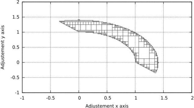
f1(x,y) = (x2+y2,x+y), R1= [−1,2]2, P1= [1,2] × [1,4]
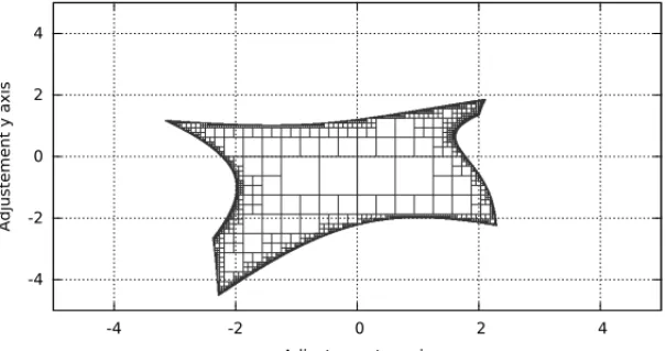
f2(x,y) = (x2−y2,
y
1+x), R2= [0,6] × [−10,10], P2= [0,5] × [−4,4].
(6.2)
Those examples have been chosen to give examples of addition, subtraction, product and division transfers fromRtoIR, and to exhibit the difference between the usual Minkowski arithmetic
and the algebraic one [2]. The calculations with theψ-algorithm are shown on Figures 3, 4 and 5. The convergence to 0 or 1 probabilities only, shows that inclusion functions are well constructed and that the pseudo-interval arithmetic is robust. The following example
f3(x,y)=(x2−y2·exp(x)+x·exp(y),x·(x+y)−y2), R3=P3= [−5,5]2 (6.3)
presented on Figure 5 shows clearly that the ψ-algorithm implemented in the algebraic arith-metic we use is not data dependant. The variables appear more than once in the formal expres-sion of the function f3. The CPU time for this inversion is about 255 seconds on a simple 1.67
There is no limitation for the dimensions of the adjustments and performances sets as shown on Figure 6 for the function f4:R3−→R4.
-4 -2 0 2 4
-4 -2 0 2 4
Adjustement y axis
Adjustement x axis
Performance preimage set
Figure 5:ψ-algorithm for f3.
Figure 6:ψ-algorithm for f4(x,y,z)=(x,y,z,x2−y2+z2)withR4= [−5,5]3andP4= [−10,10]4.
Due to the bisection, the algorithm computational complexity is exponential according to the iterationsN, and it is not improved compared to SIVIA one. In our scheme, computational time is defined as
Tcom p=O(N)=k·2N. (6.4)
However, if the native function is differentiable onRn, it is possible to define an adaptive mesh,
time constant with mean of paralleling using domain decomposition [18]. The adjustment set is divided on the first axis, and each processor performs theψ-algorithm on one of those sub-domains. The master processor collects all the results at the end of the calculations.
7 CONCLUSION
A new algebraic approach for interval arithmetic, called pseudo-interval arithmetic has been proposed. It is based on free algebra build from Minkowski products of basis intervals and with dimension higher or equal to 4. One has identified intervals with the elements of this associative algebra and showed that their product is distributive with respect to their addition. Increasing the dimension will give pseudo-intervals product closer to Minkowski one’s.
One has presented also a heuristic way to transfer real functions to inclusion ones depending on the space needed (semi-group or vector space). This permits to define a simple but very ef-ficient algorithm for set inversion, theψ-algorithm, which uses pseudo-intervals arithmetic and probability calculations. The convergence of this algorithm is guaranteed, and it offers several possibilities of applications, such as solving algebraic equations, differential equations, proba-bility law of random variables calculations (discrete or continuous), topological analysis, numer-ical Lebesgue integrals computations, data analysis such as principal components analysis, and parameters identification.
ACKNOWLEDGMENTS
The author thanks Michel Gondran from University of Paris-Dauphine and Thierry Socroun from Electricity of France for useful and helpful discussions.
RESUMO.Neste artigo, apresenta-se como usar um novo arcabouc¸o de aritm´etica intervalar com base na construc¸˜ao de ´algebra livre, chamado pseudo intervalos, que ´e associativa e
dis-tributiva e permite a construc¸˜ao da inclus˜ao de func¸˜ao bem definida para semi-grupo intervalar
e para seu espac¸o vetorial associado. Apresenta-se oψ-algoritmo (Invers˜ao Probabil´ıstica de Conjuntos), que realiza a invers˜ao de func¸˜oes e exibe-se alguns exemplos num´ericos.
Palavras-chave: Algebra livre, Pseudo-intervalos e aritm´etica intervalar, conjunto de in-´
vers˜ao, probabilidade.
REFERENCES
[1] A. Kenoufi, J.F. Osselin & B. Durand. System adjustments for targeted performances combining symbolic regression and set inversion, in “Inverse problems for science and engineering”, (2013), DOI: 10.1080/17415977.2013.790384.
[2] Nicolas Goze. PhD Thesis, “n-aryalgebras and interval arithmetics”, Universit´e de Haute-Alsace, France, March (2011).
[4] N. Wiener.Proc. of the London Math. Soc.,19(1921), 181–205.
[5] P.S. Dwyer. Linear Computations, John Wiley & Sons, Inc., 1951, chapter Computation with Approx-imate Numbers.
[6] Mieczyslaw Warmus. Calculus of Approximations. Bull. Acad. Pol. Sci. C1. III, IV(5) (1956), 253–259.
[7] Mieczyslaw Warmus. Approximations and Inequalities in the Calculus of Approximations. Classifi-cation of Approximate Numbers. Bull. Acad. Pol. Sci. Math. Astr. & Phys.,IX(4) (1961), 241–245.
[8] R.E. Moore. Interval Analysis I by R.E. Moore with C.T. Yang, LMSD-285875, September 1959, Lockheed Aircraft Corporation, Missiles and Space Division, Sunnyvale, California.
[9] R.E. Moore. Interval Integrals by R.E. Moore, Wayman Strother and C.T. Yang, LMSD-703073, 1960 Lockheed Aircraft Corporation, Missiles and Space Division, Sunnyvale, California.
[10] R.E. Moore. Ph.D. Thesis, Stanford, (1962).
[11] R.E. Moore. Interval Analysis (Prentice Hall, Englewood Cliffs, NJ, 1966) on this topic. Almost nobody was willing.
[12] R.E. Moore. A test for existence of solutions to nonlinear systems. SIAM J. Numer. Anal., 14(4) (1977), 611−615.
[13] R.E. Moore. Interval Analysis. Prentice Hall, Englewood Cliffs, N.J., (1966).
[14] S.M. Markov. Isomorphic Embeddings of Abstract interval Systems.Reliable Computing,3(1997), 199–207.
[15] S.M. Markov. On the Algebraic Properties of Convex Bodies and Some Applications.J. Convex Anal-ysis,7(1) (2000), 129–166.
[16] R.E. Moore, R.B. Kearfott & M.J. Cloud. Introduction to interval Analysis, SIAM, Philadelphia, January, (2009).
[17] W.H. Press, S.A. Teukolsky, W.T. Vetterling & B.P. Flannery. Numerical Recipes in C: The Art of Scientific Computing, 2nd Ed., Cabridge University Press, New York, (1992).
[18] L. Jaulin, M. Kieffer, O. Didrit & E. Walter.Introduction to interval analysis. SIAM. 2009 Applied interval Analysis. Springer-Verlag, London, (2001).
[19] http://www.ti3.tu-harburg.de/rump/intlab/
[20] R.B. Kearfott. Rigorous Global Search: Continuous Problems, Kluwer Academic Publishers, (1996).
[21] Numerica: A Modeling Language for Global Optimization by Pascal Van Hentenryck, etc., Laurent Michel, Yves Deville, MIT Press, (1997).
[22] A. Kenoufi.Differential calculus and linear algebra in pseudo-intervals free algebra, Preprint, Strasbourg, (2013).
[23] J.A. Nelder & R. Mead. “A simplex method for function minimization”.Computer Journal,7(1965), 308–313.
[24] M. Goze & N. Goze.Arithm´etique des intervalles Infiniment Petits. Preprint Mulhouse, (2008).
[25] N. Goze & E. Remm. An algebraic approach to the set of intervals, arXiv:0809.5150, (2008).
[27] http://www.python.org.
[28] http://www.sagemath.org.
[29] http://maxima.sourceforge.net.
[30] A.S. Householder. The theory of matrices in numerical analysis, Dover Publications, Inc. New-York, (1975), p. 9.
[31] http://www.scilab.org.
[32] S.M. Markov. Extended Interval Arithmetic Involving Infinite Intervals. Mathematica Balkanica, New Series,6(3) (1992), 269–304.
[33] S.M. Markov. On Directed Interval Arithmetic and its Applications.J. UCS,1(7) (1995), 510–521.
[34] S.M. Markov. On the Foundations of Interval Arithmetic. In: Alefeld G, Frommer A & Lang B. (Eds.): Scientific Computing and Validated Numerics Akademie Verlag, Berlin, pp. 507–513.
[35] S.M. Markov. Isomorphic Embeddings of Abstract Interval Systems.Reliable Computing,3(1997), 199–207.
[36] T. Sunaga. Theory of Interval Algebra and its Applications to Numerical Analysis.RAAG Memoirs, 2(1958), 29–46.
[37] H.-J. Ortolf. Eine Verallgemeinerung der Intervallarithmetik. Geselschaft fuer Mathematik und Datenverarbeitung, Bonn 11, (1969), pp. 1–71.
[38] N. Dimitrova, S.M. Markov & E. Popova. Extended Interval arithmetic: New Results and Appli-cations. In: Atanassova L & Herzberger J. (Eds.): Computer Arithmetic and Enclosure Methods. Elsevier Sci. Publishers B.V., (1992), pp. 225–232.
[39] E.D. Popova. Multiplication Distributivity of Proper and Improper Intervals.Reliable Computing, 7(2) (2001), 129–140.
[40] E.D. Popova. All about Generalized Interval Distributive Relations. I. Complete Proof of the Rela-tions. Sofia, March (2000).
[41] E. Popova. On the Efficiency of Interval Multiplication Algorithms. Proceedings of III-rd Interna-tional Conference “Real Numbers and Computers”, Paris, April 27-29, (1998), 117–132.
[42] E. Kaucher. Ueber metrische und algebraische Eigenschaften einiger beim numerischen Rechnen auftretender Raume. Dissertation, Universitaet Karlsruhe, (1973).
[43] E. Kaucher. Algebraische Erweiterungen der Intervallrechnung unter Erhaltung der Ordnungs und Verbandstrukturen Computing, Suppl. 1, (1977), pp. 65–79.
[44] E. Kaucher. Ueber Eigenschaften und en der Anwendungsmoeglichkeiten der erweiterten Intervall-rechnung und des hyperbolischen Fastkoerpers ueber R Computing, Suppl. 1, (1977), pp. 81–94.
[45] E. Kaucher. Interval Analysis in the Extended Interval Space IR Computing, Suppl. 2, (1980), 33–49.
[46] E. Gardenes & A. Trepat. Fundamentals of SIGLA, an Interval Computing System over the Com-pleted Set of Intervals.Computing,24(1980), 161–179.
[47] E. Gardenes, A. Trepat & J.M Janer. SIGLA-PL/1 Development and Applications. In: Nickel K.: Interval Mathematics 1980, Academic Press, (1980), 301–315.
[49] E. Gardenes, A. Trepat & H. Mieglo. Present Perspective of the SIGLA Interval System. Freiburger Interval-Berichte 82/9, (1982), 1–65.
[50] E. Gardenes, H. Mielgo & A. Trepat. Modal intervals: Reason and Ground Semantics, In: K. Nickel (Ed.): Interval Mathematics 1985, Lecture Notes in Computer Science, Vol. 212, Springer-Verlag, Berlin, Heidelberg, (1986), 27–35.
[51] E. Gardenes, M.A. Sainz, L. Jorba, R. Calm, R. Estela, H. Mielgo & A. Trepat. Modal Intervals,