Inflationary Inertia:
A New Estimation of the
Phillips Curve For Brazil
Angelo Marsiglia Fasolo Research Department (DEPEP), Banco Central do Brasil Marcelo Savino Portugal Professor of Economics at Federal University of Rio Grande do Sul (UFRGS) and associate researcher of CNPq
RESUMO
O artigo estima uma nova relação entre emprego e inflação para o Brasil, tendo como pano de fundo hipóteses novo-keynesianas. Quatro hipóteses são testadas e sustentadas: i) os agentes não possuem racionalidade perfeita; ii) a imperfeição na formação das expectativas pode ser determinante no componente inercial da inflação brasileira; iii) a inflação possui componente inercial autônomo; e, iv) relações não-lineares entre inflação e desemprego for-necem melhores resultados para a economia nos últimos 12 anos. Enquanto as duas primei-ras hipóteses são verificadas por meio de modelo com mudanças markovianas, as últimas são testadas por uma Curva de Phillips convexa, estimadas pelo Filtro de Kalman. O uso des-tas estimativas não prejudica as propriedades tradicionais estimadas de funções de resposta da política monetária para o Brasil.
PALAVRAS-CHAVE
curva de Phillips, expectativas, inflação, hiato do desemprego, modelos markovianos, filtro de Kalman, SUR
ABSTRACT
This paper presents some new estimates for the relationship between inflation and unem-ployment in Brazil based on a new Keynesian hypothesis about the behavior of the economy. Four main hypotheses are tested and sustained throughout the study: i) agents do not have perfect rationality; ii) the imperfection in the agents expectations generating process may be an important factor in explaining the high persistence (inertia) of Brazilian inflation; iii) infla-tion does have an autonomous inertial component, without linkage to shocks in individual markets; iv) a non-linear relationship between inflation and unemployment is able to provide better explanations for the inflation-unemployment relationship in the Brazilian economy in the last 12 years. While the first two hypotheses are tested using a Markov Switching based model of regime changes, the remaining two are tested in a context of a convex Phillips Curve estimated using the Kalman filter. Despite the methodological and estimation im-provements provided in the paper, the impulse-response functions for the monetary policy presented the same properties shown in the literature that uses Brazilian data.
KEY WORDS
Phillips curve, expectations, inflation, NAIRU-gap, Markov switching models, Kalman filter, SUR
JEL Classification
INTRODUCTION
The relationship between aggregate demand and inflation has been the ob-ject of extensive research and discussion in economics. Since the seminal work of Phillips (1958), several formulations have attempted to establish a relationship between the oscillations in price and employment levels, by using a consolidated economic theory consistent with the microfoundati-ons. A consensus seemed to be emerging with the “New Keynesian Phillips Curve”, referred to by McCallum (1997) as “the closest thing there is to a standard formulation.” Although discussions date back to the mid-90s, the “New Keynesian Phillips Curve” originates from Taylor (1980) models. More than conveniently, staggered contracts also contribute to the New Keynesian theory construction, as their existence does not allow rejecting the optimization hypothesis for the individual behavior of agents.1
Nonetheless, some questions are raised about the consistency of such a the-ory. Roberts (1997), especially, argues that the Phillips Curve, generated by the sticky-inflation model and rational expectations, exhibits lesser data ad-justment than a sticky-price model, due to the supposedly imperfect rationa-lity of the agents as to their expectations formation. Therefore, the issue now is whether there is inflation inertia in function of the contracted values or whether, in fact, it is the price level that shows persistence as a result of imperfect expectations. Another aspect that should not be overlooked is the relationship with supply shocks. Some authors, especially Ball and Mankiw (1995), are not satisfied with the microfoundation of supply shocks and their spread in aggregate price levels led to formulations and tests with quite peculiar control variables, in which higher-order statistical moments of price level components were associated with the menu cost theory.
between inflation and expectations through Markov models and the estima-tion of the Phillips Curve then includes New Keynesian issues. Finally, mo-netary policy reaction functions are estimated by a system of equations whose core is the estimated relationship between inflation and unemploy-ment. In section 1, the literature is reviewed, with a brief discussion on how to extract expectations from the agents; afterwards, results follow, as well as the methodology of other studies. Section 2 describes the theory of current formulations for the Phillips Curve, focusing on empirical inconsistencies, as well as on the econometric procedure adopted. Section 3 develops the proposed topics, while last section concludes.
1. INFLATION EXPECTATIONS AND THE PHILLIPS CURVE
This section presents empirical results regarding the analysis of expectations, their measure and their narrow and quite recently investigated relationship with the Phillips Curve. After this relationship is established, some results obtained as to the dynamics between inflation and unemployment are pre-sented, with special emphasis on the econometric method used and the me-asure of the adopted expectation.
1.1 Composition and Analysis of Expectations
while, in England, one is conducted by the Gallup Organization with over one thousand employees.2
The estimation of stochastic processes for inflation takes for granted that agents bear an “econometric model” in mind, opening up a world of infinite possibilities, such as univariate or multivariate models, long or short lags, etc (see BALL, 2000). For Brazil, there is a problem with the determination of the behavior of agents due to structural breaks. The most common arbi-trage strategies when estimating Phillips Curves use past inflation as proxy for inflation expectations. As Ball (2000) interestingly puts it, quoting Sar-gent (1999), aSar-gents do not know a priori about inflation behavior; instead,
they go through a constant learning process, implying the necessity of mo-dels that mimic human learning skills. In some way, this is the procedure adopted when working with artificial neural networks.3
Bonds traded on financial markets are largely used to measure inflation ex-pectations. Apparently, this method has fewer limitations and may be used without further hypotheses about the behavior of agents.4 The use of the term structure is justified by Fisher’s identity, where the nominal rate on a bond corresponds to the real rate plus the expected inflation rate at the end of the bond’s term. Nevertheless, its use involves some important assumpti-ons: i) functioning of the Expectations Hypothesis;5 ii) nonexistence of
mo-netary policy shifts during the maturity of the considered bonds; iii) same default risk component and liquidity, regardless of maturity dates, in bonds of the same country.
Thus, consider a pre-fixed interest rate bond for the first working day of month t and a post-fixed interest rate one for the last working day of t, both
with the same maturity. For the pre-fixed interest rate bond, Fisher’s identi-ty proposes that:
2 In Brazil, the Central Bank has started conducting a survey in April 1999. Therefore, the sam-ple size is not sufficient for reliable inferences. The data are collected from financial institutions. 3 About the use of models that presume limited rationality of the agents, see the classic work of
SARGENT (1993.)
4 In the empirical section, developed in section 3, the measure of expectation is based on this method.
(1)
The post-fixed interest rate bond can be decomposed in the expectations about monetary policy (real interest rates) plus the correction of an inflation rate:
(2)
Supposing that the monetary policy does not change along the maturity term (E(rt) = rt), we have:
(3)
In the analysis of the interaction between inflation and expectations, the li-terature points out the difference to what was expected by perfect rationality assumptions, consequence of the persistence of expectations. However, data contain more information about future inflation than the simple extrapolati-on of past values.6 Some justifications are based on assumptions about Ma-rkov processes for inflation, as in Dahl and Hansen (2001), or on the absence of credibility to the monetary authority, as stated by Ragan (1995) and Gagnon (1996).
1.2 The Applications of Phillips Curve
Perhaps the most practical result of the Phillips Curve estimation concerns the measure of the natural rate of unemployment, or the non-accelerating rate of unemployment (NAIRU, for linear curves). The validity of such a
re-presentation is still in discussion. The constant shifts of the curve in the 1970s raised questions about the relationship between inflation and unem-ployment. It made Staiger, Stock and Watson (2001) divide economists in two groups: “theories in which ‘the Phillips Curve is alive and well, but’... and those that proclaim that ‘the Phillips Curve is dead’.” (p. 2). As it will be sho-wn, the statements made by the first group make more sense: the Curve is
6 See, for instance, RAGAN (1995), GAGNON (1996), ROBERTS (1997), BROUWER and ELLIS (1998).
( ) ( e)
t t
pre
t r
i = 1+ *1+π
( t ) ( t)
post
t E r
i = 1+ ( ) * 1+π
well established as theoretical representation, although it should incorporate properties considered by modern macroeconomics.
Another important distinction is between two inexplicably exclusive objecti-ves in the Curve’s applications. Some authors7 are concerned with the
esti-mation of the NAIRU itself, measuring the excess demand and laying aside assessments of the monetary policy. Other authors8 are only concerned with
the theory of monetary policy, trying to verify the consistency of the Phillips Curve as theoretical construct, using different measures of activity in an at-tempt to check the empirical robustness of results.
Estimations of New Keynesian models are presented in Roberts (1995, 2001). The Phillips Curve is tested with different measures of expectations and economic activity. To the former, the author used the University of Mi-chigan survey, the Livingston Survey and the observed future inflation. To the
latter, he used unemployment, capacity utilization and detrended output. The estimation is made with instrumental variables, with oil price fluctuati-ons and government spending as instruments, in addition to a dummy vari-able with unit value when the US president was a democrat one. The inclusion of additional inflation lags to correct specification problems raises some doubt on the perfect rationality assumption.
In an attempt to incorporate short-term NAIRU properties, some authors use techniques that can identify changes to the excess of demand over the ti-me. Gordon (1996) estimates the traditional Phillips Curve, allowing NAI-RU to follow a random walk. The estimated model is as follows:
πt = a(L)πt + b(L)(Ut – U*t) + c(L)zt + ut (4)
U*t = U*t-1 + εt ,
7 In line with this group we have GORDON (1996), STAIGER, STOCK and WATSON (1996, 2001), DEBELLE and LAXTON (1997), PORTUGAL and MADALOZZO (2000), TEJADA and PORTUGAL (2001) and LIMA (2000).
where U*t is the natural rate at instant t, zt is a vector of control variables, Ut is the rate of unemployment and x(L) is a lag polynomial. Note that if
the variance of the second equation is equal to zero, the model converges to the traditional analysis, with a non-time-varying NAIRU, a hypothesis that is rejected in the present study. The estimation is made by way of Gaussian maximum likelihood (see HAMILTON, 1994). The measurements are sta-ble in subsamples and have very narrow confidence intervals. The concavity hypothesis is rejected in favor of the linear formulation.
Gordon (1996) is a response to Staiger, Stock and Watson (1996), who pre-sented high confidence intervals (the NAIRU for 1990 would oscillate be-tween 5.16% and 7.24%). Their estimation used the random walk hypothesis for inflation, where expected inflation corresponds to the past one and did not allow the NAIRU to vary, which could be the source of inaccuracy. In spite of this, the authors make it clear that unemployment has considerable power to forecast the inflation rate.
changes. The model is the same as in Gordon (1996), but it is the constant that varies, not the measure of economic activity. The results accept the vali-dity of the Curve. Yet, it is stressed that movements of wages, prices and unemployment should focus on understanding the univariate trends, becau-se of the instability of parameters over time.
For Brazil, three studies are of note due to their econometric methodology. Portugal and Madalozzo (2000) use two processes for calculating the NAI-RU. The first one is based on the transfer from a Phillips Curve. Assuming that, in periods of high inflation, mistakes are highly costly, the authors use an ARIMA model forecasting as expectations. The second method is the es-timation of structural components of unemployment. The main idea is to eliminate short-term determinants, having the remaining forecast as measu-re of the NAIRU. The authors measu-reject this methodology, since it did not allow the existence of a residual for economic activity that explains the dy-namics of inflation.
2. THE PHILLIPS CURVE THEORY AND ECONOMETRIC METHO-DOLOGY
The modern version of the Phillips Curve combines the foundation of indi-vidual behavior and the relationships between the economic aggregates into the same theoretical framework, attempting to justify the presence of nomi-nal price rigidity and inflation inertia in the agents’ choices. Assuming mo-dels based on staggered contracts (TAYLOR, 1980), where contracts become the origin of short-term price rigidity, we derive the Phillips Curve based on Roberts (1997).9 Afterwards, we show the compatibility of the
sticky inflation model with rational expectations (FUHRER and MOORE, 1995), with the sticky price model, in addition to the relaxation of the ex-pectations hypothesis, as proposed by Roberts (1997).
Taylor (1980) assumes two-period contracts. Then, the mean wage paid by the firms is:
(5)
where xt is the contract wage chosen in t for periods t and t+1. Considering
that workers are concerned with a measure of demand (e.g. unemployment,
Ut) and that ptis the price level at t, we have as job offer (k is a constant):
(6)
Assuming firms in monopolistic competition, a normalized wage markup to zero is supposed (pt = wt). Combining this with (5) and (6) and
defi-ning πt = pt – pt-1, inflation rate at t is:
(7)
9 It is possible to prove that the model developed by CALVO (1983) produces the same set of equations as a result. For demonstrations, see WALSH (2000, pages 218-220).
( + −1)/2
= t t
t x x
w
( )
t t e
t t
t k U
p p
x − + + = −α +ε 2
1
( ) 2( ) ()
2
4 1 1
1 k Ut Ut t t Error t
e t
t−π+ = − α + − + ε +ε− −
where Error(t) = πt - πt defines an expectation error for the current
inflati-on.10 Except for Error(t), this is the Curve equivalent to the traditional
for-mulation. Hereinafter, Error(t) will be defined as ex-post bias, as in Dahl and
Hansen (2001), to distinguish it from statistical forecast error. The ex-post bias reflects the attributed probability to the regime switch of inflation be-tween t-1 and t, assuming that it follows a Markov process. For the authors,
the agents know the current regime only during the transition period. The-refore, attributing a probability other than zero for regime switch causes a bias in expectations.
Fuhrer and Moore (1995) change equation (6), by supposing that workers do not perceive the real wage levels, but the variations of real wages obtai-ned in the previous period. The equation, with kt as a constant, becomes,
(8)
Note that real wage is the mean between real wages in the previous period and the expectations for the end of the contract, adjusted according to the economic activity. Therefore, the authors rewrite (8) as:
(9)
where Δxt = xt – xt-1. Considering the price markup and combining
equati-ons (8) with (5):
(10)
which is the same equation (7) above, but with variation of inflation and expectations as endogenous variable. Roberts (1997) rewrites equation (10) as follows:
10 Apparently, the error would be in the price level. However, by adding and subtracting the price level at t, we obtain the rate of inflation subtracted from the expected rate – hence, the forecast
error.
( ) ( 1 1) ( 1 1) ' ' ,
2 t t
e t t t
t t
t k U
p x p
x p
x − = − − − + + − + + −α +ε
( 1) ' ' ,
2 t t
e t t
t k U
x − π +π = −α +ε
Δ +
( ) 2( ) ( )
' 2 '
4 , 1
, 1
1 k Ut Ut t t Error t
e t
t−Δ = − + + + −
(11)
The left-hand side is modified to provide an error in inflation forecast, so that part of the equation consists of rational expectations and the remaining of past extrapolation. Thus, Fuhrer and Moore (1995) include in their mo-del both the sticky inflation, with rational expectations, and the sticky price formulation, with agents of different expectation formations. Interestingly, the endogenous variable in (11) does not express a “forecast error”, as Ro-berts (1997) suggests. Its best definition may be the difference between in-flation and state of expectations, as “average expectation” is actually formed by past values and the future expectation. Even considering agents with di-fferent expectation formations, nothing assures the same proportion. The sense ascribed by the author may be more appropriate as ex-post bias. Despite the consensus, some topics are unclear in empirical investigation and in theory implied by the Phillips Curve. Two aspects criticized are infla-tion inertia and the economy’s behavior in disinflainfla-tion. According to Fuhrer and Moore (1995), the inertia in Taylor (1980) is restricted to the adjust-ment period of output to equilibrium, which is lower than verified.11 Ball
(1994, 1995) shows the chance of economic growth as result of credible de-flations. The issue relates to the adjustment of expectations: if they have the necessary speed, excess demand does not influence the prices. Mankiw and Reis (2001) cite the “flexibility of expectations” to justify their result. Galí and Gertler (1999) show that the model assumes positive correlation be-tween the variation of contemporaneous inflation and the output gap in the future. However, empirical data show an inverse pattern.
Fuhrer and Moore (1995) is one of the variations that tries to correct origi-nal problems. Others (ROBERTS, 1997 and 1998, BALL, 2000) make in-ferences about expectations, in line with Bonomo, Carrasco and Moreira (2000), which include notions of evolutionary games. In cases of disinflati-ons, regardless of credibility, agents choose between adjusting prices and
ke-11 ERCEG and LEVIN (2001) cite studies where inflation persistence coincides with unstable policies. GORDON (1996) concludes that the American inflation is “dominated” by inertia. CATI, GARCIA and PERRON (1995) find a random walk of the Brazilian inflation in the period that preceded the Real Plan.
( ) ( ) ( )
2 ) ( 2
' 2
' 2
, 1 , 1 1
1 k U U Error t
t t t t e
t t
t + + −
+ − = +
− π − π + α − ε ε−
eping the old strategy. Occasional “myopia” causes losses proportional to the length of the adaptive strategy. Mankiw and Reis (2001) justify “myo-pia” by the amount of information the agents receive, since there are costs for obtaining them to improve estimation of future inflation. Carroll (2001) questions this model, as most agents obtain information at low cost from newspapers. He develops a model based on epidemiological studies, where the sluggish adjustment of expectations is justified by the exposure to the news. For Brazil, Almeida, Moreira and Pinheiro (2002) replicate Roberts (1997) with a sample from 1990 to 1999, finding evidence in favor of Fuhrer and Moore (1995). One could criticize their sample, since the two-stage estimator (2SLS) has only asymptotic consistency. Besides, there is no inference about expectations at all, imposing the future value as the agents’ expectations.
2.1 Asymmetry of Prices and Supply Shocks:
Controlling exogenous supply shocks is left as a complement imposed by the researcher. The classical approach uses a set of relatively inelastic supply products. After choosing the set, two options are available: to remove the products from the price index (forming a “core”), or to include the variati-ons as explanation for the model. Criticisms about the use of disaggregated indices lie in the incapacity to eliminate the spread of shock from a sector to the whole economy. Adding lags to the equation avoids this problem. Examples of series used are changes in oil price, imported goods’ price (see GORDON, 1996) and changes in the price of some types of foods (see STAIGER et alii, 1996 and MIO, 2001).
inflation, with loss of significance of the basket of products when the asym-metry and kurtosis variables are added.
Mio (2001) uses the asymmetry of Japanese data and confirms the hypothe-sis above about the efficiency of this control. The author relates inflation inertia to the asymmetry of the distribution, affirming that the persistent price fluctuations are only due to the spread of shocks on economic sectors, without an “autonomous” inertial component. If the shocks are fully respon-sible for inflation inertia, their spread corresponds to the remaining asymme-tries. The author’s measure of asymmetry has interesting properties, as it consists of the difference between the headline and the trimmed inflation:
(12)
where πt
30%is the inflation rate trimmed at 30% on each tail,ω
itis the
wei-ght of item i in period t, N is the number of items that form the total price
index and M is the number that remains after exclusion.12 The result is the
sum of the extreme components of the distribution, thus representing a me-asure of asymmetry. We observe two aspects regarding supply shocks captu-red by this measure: the measure of the shock itself (the more asymmetric the distribution, the more sectors will be in extreme situations), and shock persistence. It is also underscored that the variable strongly controls the components of IPCA (extended CPI) on a regular basis, such as seasonality. In fact, Ball and Mankiw (1995) and Mio (2001) use full-price indexes and do not control the regressions made with seasonal factors. The measures of elevated statistical moments accomplish this task.
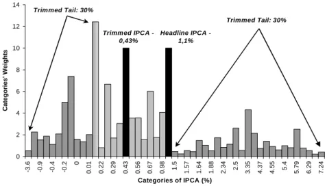
Abrupt changes in relative prices, a special kind of supply shock, can be con-trolled by the SKEW variable. Figure A shows the distribution of 47 items
of IPCA in March 1999. The black bars show the headline IPCA (1.1%) and the 30% trimmed mean (0.43%). The large difference between these two values is due to the distribution of the extreme price variations. It is 12 The choice of the mean with 40% of the core of IPCA is based on FIGUEIREDO (2001). The author points out that this cut tends to value the effects of asymmetry, which is the measure desired as control variable for Brazil.
∑ ∑ ∑
= =
=
− =
−
= M
j jt M
j jt jt N
i it it t
t t
SKEW
1 1 1
% 30
ω π ω π
ω π
worth noting that, in March 1999, Brazil experienced the worst moment of the currency crises started in January that year. The exchange rate devaluati-on had a more significant impact devaluati-on prices of tradable goods, therefore in-troducing a large asymmetry in the inflation index.
FIGURE A CROSSSECTIONAL INFLATION DISTRIBUTION -MARCH 1999
2.2 Methodology and Test Equations:
Section 3 consists of three parts. In the first part, we assess the relationship between inflation and expectations by means of regime switching models. The second part estimates the New Keynesian Phillips Curve, using the Kal-man filter. In the third part, the curve is the center of a system that allows for impulse-response functions. Before these parts, issues about the stationa-rity of data are evaluated by ADF and Phillips-Perron tests, in addition to the comparison of the results with other studies. The comparisons are ne-cessary in view of the small sample available and the low power of tests adopted.
The rationality test improves the procedure of Bakhshi and Yates (1998) and Grant and Thomas (1999) which verifies whether, on average, the ex-pected inflation is an unbiased and efficient estimation of the observed infla-tion, through a cointegration vector with the following format:
FIGURE A - Cross-Sectional Inflation Distribution - March 1999
0 2 4 6 8 10 12 14 -3 .6 -0 .9 -0 .4 -0 .2 0 0. 01 0. 22 0. 29 0. 43 0. 56 0. 67 0.
98 1.5
1. 57 1. 64 1. 88 2.
34 2.5
3.
35
4.
37
4.
55 5.4
5. 79 6. 29 7. 24
Categories of IPCA (%)
Cat e gor ies' W e ight s
Trimmed Tail: 30%
Trimmed Tail: 30% Trimmed IPCA -
0,43%
(13)
whereπe
t is the expected inflation for t with information of t-1 and ut is a
white noise. Rational expectations suppose thatα and β should respectively
value 0 and 1. Note that (13) can also be written as:
(14)
supposing that β is equal to the unit. Thus, the ex-post bias can be viewed
as a white noise with a constant, whereα expresses the probability attribu-ted to the regime switch between t-1 and t. This format is more interesting,
once a stationary AR representation indicates the long-term behavior of the bias. The presence of rational expectations where the ex-post bias is syste-matized may seem contradictory, as the classic hypothesis characterizes it as a white noise with zero mean and constant variance. However, the AR esti-mation implies convergence to the mean of the process, plus a white noise. So, the bias in the present may be autocorrelated with the past, in some la-gs. However, in the long run, parameter α, discounted from short-term effects, represents the mean of the ex-post bias.
The ex-post bias equation with Markov switching assumes a single format, where the mean, the autoregressive terms and the variance of the process are liable to changes around three regimes:13
(15)
13 Models with changes to only some components (mean or variance) were unsuccessfully tested. Probably, changes to the AR terms are the reason for rejection of alternatives due to the prob-lem with residual autocorrelation.
t e t t =α+βπ +u π t e t t u t
Error()=π −π =α +
The estimation of the Markov process allows the correction of discrepant events. The use of dummy variables for shocks is mostly a restricted activity since it is not possible to reach all the components of the model (e.g. the va-riance of the regression). The use of Markov models reduces the restriction, allowing the estimation of different components in different regimes. Ano-ther advantage is the tendency for more parsimony than its linear counter-part, as shown by Clemens and Krolzig (2001).
MS-VAR estimation includes discrete Markov chains separating different and unobservable M regimes. Consider the joint density of an Yt series and
of St and St-1regimesas the product of marginal and conditional densities of
the processes:
(16)
Integrating the density functions for all possible current and past regimes, the likelihood function assumes the following format for the whole sample:
(17)
According to Kim and Nelson (2000), the function is the mean of conditio-nal densities, with transition probabilities as weights. For an AR(p) process,
the transition probability of the regime is defined as conditional to the in-formation set and the previous period regime. It distinguishes MS-VAR from other threshold models, where the threshold which determines whe-ther the process is in a certain regime is constant in the sample. In the MS-VAR model, it changes as information set increases. Hence:
(18)
For estimation of the joint probability of Stand St-1, EM algorithm, used in
Hamilton (1990) for unobservable regimes, is similar to the Kalman filter, and consists of two steps. In the forecast, the algorithm derives the transition
probability given the set of information on the past:
(Yt,St,St−1|Yt−1,St−1)=f(Yt |St,Yt−1,St−1) (*f St,St−1|Yt−1,St−1)
f ( ) [ ] ∑ ∑ ∑ = = −= − − − − − ⎭ ⎬ ⎫ ⎩ ⎨ ⎧ = T t M St M St t t t t t t t
t S S Y S S Y S
Y f L
1 0 1 0
1 1 1 1
1, Pr , | ,
, | ln
ln
{ } { }
(
| ,)
Pr( | ,β)Pr 1 1 −1
∞ = − ∞
=
−j j t j j = t t
t
t S Y S S
Pr[St = j , St-1 = i | Yt-1 , St-1] = Pr[St = j | St-1 = i].Pr[St-1 = i | Yt-1 , St-1] (19)
The first term on the right-hand side is the transition probability, whereas the second is the transition probability in the previous period. In updating
process, the probabilities’ forecast error is incorporated for future steps. So, the filter obtains two types of probability: the smoothed one, containing all information on the sample, and the filtered one, using the available infor-mation up to the time of estiinfor-mation.
The estimation of the Phillips Curve is carried out according to Debelle and Laxton (1997), with a model based in equation (11). Developing (11) to-gether with the control variables, we have:
(20) (21) (22)
Therefore, the constant represents the fixed γ parameter that weights the
unobservable componentγ*. The variable used to measure economic activi-ty is therefore the inverse of the unemployment, while the NAIRU is the re-sult of the ratio between the negative of γ* and γ. This equation’s format assumes strict convexity in the inflation-unemployment plane.
The assignment of initial values to the filter requires some care, due to the need of convergence of the algorithm with the necessary flexibility to obtain better values. Here, the estimation by OLS is adopted as initial values. The method has good rate of convergence, even though the presence of regime switching may lead to the use of inappropriate values. The correction is made with the use of the first k observations only, where k corresponds to
the number of parameters in the observation equation.14
14 The availability of data from 1990 onwards makes the initial variance increase due to Collor I Plan. Thus, the sample itself behaves like the use of a diffuse Bayesian prior for initial values.
( ) t t t t t t t e t t SKEW u u NAIRU ε β γ γ π α απ
π = + * −1+ * − + 1 +
( ) t t t t t t t t e t t SKEW u u u NAIRU ε β γ γ π α απ
π = + −1 + − + 1 +
* *
( ) t t
t t t t e t t SKEW u
NAIRU γ β ε
γ π α απ
The system estimated in the last part of section 3 uses Zellner’s method, es-timated by Full-Information Maximum Likelihood (FIML), for correction of the elevated correlation between the residuals of different equations. VAR estimation, which is traditional in the area, was abandoned because of this problem and of the use of a different set of variables in inflation equation.
3. A NEW KEYNESIAN PHILLIPS CURVE FOR BRAZIL 3.1 Preliminary Considerations: Stationarity
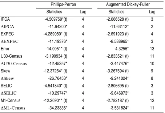
In Brazil, the analysis of stationarity is important in view of the presence of structural breaks in the economy and their influence on the behavior of vari-ables. Thus, unit root tests should take into consideration its low power, in addition to information obtained from other articles in the field. The pre-sence of a significant break in July 1994 (Real Plan) leads us to adopt the Phillips-Perron (PP) test, since the Dickey-Fuller (ADF) test has lower sta-tistical power.15 The reduced power of the unit root tests also made us
avoid their use in sample partitions, given the compromise of the assessed results, except when testing the unemployment rate.
Seven variables are used in the study: IPCA of IBGE, basic index for the in-flation targeting system; the expectations derived from interest rates ( EX-PEC); the ex-post bias, formed by the difference between these two variables; the changes of primary rate (DSELIC); the measure of skewness proposed by Mio (2001), SKEW; the open seasonally adjusted unemploy-ment rate, 30 days, of IBGE (U30-Census); and the growth rate of moneta-ry stock M1 seasonally adjusted by Census-X11 (M1-Census).
We verify that, differently from Cati, Garcia and Perron (1995), the IPCA
by the testis possibly a consequence of the small sample. Estimating the Phillips Curve, the absence of stationarity would cause damage if there were no cointegration between the variables. However, tests point to the existen-ce of more than one cointegration vector.16 In case of the system of
equati-ons, consider the observation of Hamilton (1994) about systems with nonstationary series, where the use of series in difference would throw away long-term information of the data.17
TABLE A – UNIT ROOT TEST
Note: (*) indicates rejection of the null hypothesis at 1%. “Lag” indicates the number of lags used in the test statistics. (t) indicates the use of deterministic trend and intercept in the test equation.
Results in Table A leave no doubt about the ex-post bias, even though stati-onarity occurs around a trend according to the PP test. SKEW, M1-Census
and SELIC variables have the same behavior as that of inflation and expecta-16 Result available from authors.
17 About the use of systems in difference, the author states: “The drawback to this approach is that the true process may not be a VAR in differences. Some of the series may in fact have been stationary, or perhaps some linear combinations of the series are stationary, as in a cointegrated VAR. In such cir-cumstances a VAR in differenced form is misspecified” (page 652).
Phillips-Perron Augmented Dickey-Fuller
Statistics Lag Statistics Lag
IPCA -4.509759*(t) 4 -2.666528 (t) 3
ΔIPCA -11.94200* 4 -11.63112* 2
EXPEC -4.289080* (t) 4 -2.691923 (t) 4
ΔEXPEC -11.19376* 4 -8.588965* 3
Error -14.0051* (t) 4 -4.3255* 13
U30-Census -3.190934 (t) 4 -2.833521 (t) 11
ΔU30-Census -12.45257* 4 -3.447476* 10
Skew -12.37264* (t) 4 -3.267694 (t) 9
ΔSkew -26.76453* 4 -9.241024* 8
SELIC -4.541840* (t) 4 -2.806695 (t) 3
ΔSELIC -10.29747* 4 -9.646973* 3
M1-Census -12.20901* (t) 4 -2.782187 (t) 12
tions. The ADF test accepts the unit root hypothesis, whereas the PP test points to stationarity. However, the variable for control of the monetary po-licy is the first difference of the SELIC rate. Hence, as DSELIC was
statio-nary, we do not have problems with the estimation. In contrast, the PP test shows that there are high chances of stationarity of the SKEW variable and
M1 growth. Moreover, the ADF test points to stationarity at 10% of the asymmetry. Thus, the hypotheses of stationarity for SELIC variations and for asymmetry are not a strong restriction to estimation. The evidence of Pastore (1995) regarding the cointegration between rate of inflation and money stock growth sets argument.
The test on unemployment does not reject the unit root hypothesis. This re-sult is not usual in the empirical literature (see PORTUGAL and MADA-LOZZO, 2000), even when the logit transformation is applied to limited
variables.18 Using partitions of the sample does not solve the problem, since
ADF and PP tests still reject the stationarity hypothesis concerning the post-Real Plan period.19 Probably, this result represents small samples, since tests
with significantly larger samples do not endorse the result.
3.2 Analysis of Expectations
The data on the “expected inflation” variable are available at the site of the Central Bank of Brazil. The observations consist of nominal yield of pre-fi-xed CDB (bank deposit certificate) and the post-fipre-fi-xed yield negotiated, res-pectively, on the first and on the last day of each month, for the number of working days in the month. Information covers the periods from January 1990 to August 2002. The data on the post-fixed CDB consist only of the real interest rate. Thus, the spread between the pre-fixed and post-fixed rates expresses the expected inflation rate. In equation (3), it is equivalent to the inverse of the difference, without the term (1+πt).20 The inflation used to
form the ex-post bias is the IPCA, of IBGE.
18 For details about unemployment in Brazil and the data transformations used, see PORTUGAL and MADALOZZO (2000).
This composition has implications for the events of each month. Therefore, we have: i) beginning of period t: agents have information about t-1; ii)
agents form expectations about t from the available information; iii)
infor-mation on t is made available; iv) the agents adapt to information; v)
begin-ning of t+1. Note that the agents form their expectations within the same
period. The assumptions are not very strong, given the lag between collecti-on and disseminaticollecti-on of eccollecti-onomic data.
The estimation of a cointegration vector that relates inflation and expectati-ons, in line with Bakhshi and Yates (1998) and Grant and Thomas (1999), does not reject the hypothesis that the angular coefficient is equal to one. Thus, we may assume that the ex-post bias is a stationary representation. Some procedures are traditional when assessing the existence of alternative regimes. One of them is the distribution of the variable: a bimodal, or even a fat tail, distribution (see HAMILTON, 1994, p. 687), shows signs of more than one regime. According to Table B, the Jarque-Bera test is far from configuring a normal distribution for the data. The asymmetry coeffi-cient justifies this behavior.
TABLE B – DESCRIPTIVE STATISTICS – EX-POST BIAS
The evaluation also includes the estimation of the best univariate model re-presenting the stochastic process of the analyzed series. The selection of an AR(1) is due to the adjustment in terms of information criteria and serial autocorrelation. Stability tests are used to check the presence of regimes. Chow test points to the existence of a structural break in July 1994. The RESET test points to misspecification of the model at 10% with one nonli-near term. The recursive estimation shows large variance of the constant,
20 Similar applications in BONOMO and GARCIA (1997) and SCHOR, BONOMO and PEREIRA (1998).
Mean 0.460734 Median -0.022393 Jarque-Bera 33393.68
Standard deviation 3.827322 Asymmetry 7.312726 Prob. 0.000000
implying that the confidence interval, depending on the period of analysis, is quite wide.21
The “J” test of Davidson and MacKinnon (1981) was used for determinati-on of the number of regimes. The models were selected with the aim of checking three components: autoregressive dynamics, regimes and dummy variablesfor economic plans. The justification for the use of dummy varia-bles in some models is the violation of the maintenance of monetary policies in the period covered by CDBs. It is plausible to support the existence of an inflation forecast error in view of abrupt disinflation processes. Two varia-bles were adopted: one to cover the price-freeze period of Collor II Plan (February to June 1991) and another one in the months after the switch to the Real Plan (July 1994). Both have unit value for the time comprised by the event.
TABLE C – “J” TEST – NUMBER OF REGIMES
Note: “Test” reports confronted models, the first of which is a null hypothesis, while the second is the alternative. “Estimated Value” shows the estimation of the alterna-tive model in the test. “t statistics” informs the significance of the parameter.
21 Assuming a 95% interval, the constant varies from –5.77 to 4.90. This interval is unrealistic, especially after the Real Plan.
Test Estimated value t statistics Choice
Linear X MS(2)AR(1)-d1 0.636933 3.869482 MS(2)AR(1)-d1
Linear X MS(3)AR(5)-d1 1.016563 17.03038 MS(3)AR(5)-d1
MS(2)AR(1)-d1 X MS(2)AR(5)-d1 0.975699 10.78761 MS(2)AR(5)-d1
MS(2)AR(1)-d1 X MS(3)AR(5)-d1 0.994653 16.22412 MS(3)AR(5)-d1
MS(2)AR(5) X MS(3)AR(5) 1.078637 18.15003 MS(3)AR(5)
MS(2)AR(5) X MS(3)AR(5)-d1 1.017146 14.79181 MS(3)AR(5)-d1
The information criteria point to diverse results: while the SIC points to the MS(2)AR(5)22 model, the Akaike criterion converges to MS(3)AR(5)-d1. It is important to emphasize the rejection of a low number of lags, besides the need of better control of the dummy variables, since, in most tests, the Real Plan variable was not significant at 5%. Possibly, this is consequence of anti-cipation of the measures by policymakers. This way, agents showed no “sur-prise” when implementing the new currency. Table C reports the results of “J” tests, where those models with simpler specifications are rejected in fa-vor of more complex ones. An interesting result was obtained with MS(3)AR(5), as it excelled its equivalent with a dummy variable for Collor II plan. Nevertheless, this is inconsistent with the information criteria.
The estimation of the model with Markov switching and one control varia-ble (price-freeze in Collor II Plan) yielded the results in tavaria-ble D.23 The test
of Davies (1977), standard to confirm the presence of more than one regi-me, shows the acceptance of the Markov model. The information criteria also point to the superiority of the model over the linear one. The residuals do not show autocorrelation. The sensitivity test, however, captures proble-ms, for instance, in the elimination of ARCH-type residuals at 5%. The test is performed with smoothed residuals, trying, as Garcia and Perron (1996) did, to capture the presence of regime-dependent changes to the variance. In contrast, according to Kim and Nelson (2000), ARCH-type residuals were not found with the test on standardized residuals.
22 The nomenclature follows KROLZIG (1998): “MS(x)AR(y)” points to the model with “x” regimes and AR structure of “y” lags. “d” shows dummy variables in Collor II and Real Plans, “d1” shows dummy variables only in Collor II Plan.
TABLE D – ESTIMATION OF THE REGIME SWITCHING MODEL – MS(3)AR(5)-D1
Variable Coefficient Std. Error t-Statistic
Regime 1 – Standard Error: 0.13019
C (Regime 1) -0.6891 0.0507 -13.5952
AR(1) 0.6424 0.0150 42.8139
AR(2) -0.5132 0.0136 -37.7882
AR(3) 0.0168 0.0169 0.9939
AR(4) -0.1302 0.0134 -9.7302
AR(5) 0.0359 0.0191 1.8803
Collor II -0.6891 0.0507 -13.5952
Regime 2 – Standard Error: 0.48182
C (Regime 2) -0.0185 0.0495 -0.3745
AR(1) 0.5845 0.0861 6.7882
AR(2) -0.0248 0.0818 -0.3026
AR(3) 0.0897 0.0198 4.5379
AR(4) -0.0540 0.0167 -3.2403
AR(5) 0.1194 0.0151 7.9072
Collor II -4.3723 94.9852 -0.0460
Regime 3 – Standard Error: 2.1882
C (Regime 3) 1.5081 0.4551 3.3136
AR(1) -0.4969 0.1424 -3.4896
AR(2) -0.0990 0.1790 -0.5532
AR(3) -0.2933 0.1541 -1.9037
AR(4) -0.1276 0.1615 -0.7898
AR(5) -0.1270 0.1213 -1.0462
Collor II 10.5075 1.8273 5.7504
Comparison with the Linear Model:
log-likelihood: -171.2123 linear system : -292.5500
AIC criterion: 2.7376 linear system : 4.0891
SC criterion: 3.3479 linear system : 4.2519
LR linearity test: 242.6753 Chi(16) =[0.0000] ** Chi(22)=[0.0000] **
The characterization of the processes is important for the analysis. As sho-wn in Graph 1, regimes 2 and 3 determine low and high inflation regimes, respectively. Regime 2 presents low variance, nonexistence of systematic er-rors (constant indifferent from zero) and high persistence of ex-post bias. Regime 3 is characterized by underestimation of inflation and high persis-tence of ex-post bias just as in regime 2. Regime 1 captured two peaks be-tween April and June 1991 and July and August 1994. In both cases, the periods coincide with expectations that are higher than inflation, either due to the hope for the end of the price-freeze at the first peak or due to the cre-dibility regarding the July 1994 plan.
GRAPH 1 - ESTIMETED PROBABILITIES - MS(3)AR(5)-d1
Durability is one more aspect of regime 1. The transition matrix of regimes is given by:
1991 1992 1993 1994 1995 1996 1997 1998 1999 2000 2001 2002 0.5
1.0
Probabilities of Regime 1 filt ered
p redict ed
sm o ot hed
1991 1992 1993 1994 1995 1996 1997 1998 1999 2000 2001 2002 0.5
1.0
Probabilities of Regim e 2
1991 1992 1993 1994 1995 1996 1997 1998 1999 2000 2001 2002 0.5
1.0
Probabilities of Regime 3
As we may observe, the largest probability, from the moment we enter regi-me 1, is that agents tend towards the regiregi-me with higher variance and high forecast error. It is hard to speculate about learning process during crises, as the agents try to compensate for the error made with another error in the opposite direction. We verify that there is a minimally calculated probability of being in regime 1 and remaining in it, with duration of approximately one month and a half, as against a probability of 86 months in period 2. This is directly related to the time interval at which regimes occur: regime 1 was always followed by high inflation periods. The sole exception is the pe-riod between July and August 1994, when the economy entered a perma-nent phase of low inflation.
GRAPH 2 CONDITIONAL DURATION’S PROBABILITIES -MS(3)AR(5)-d1
The conditional duration’s probability, which conveys the notion of trajec-tory between regimes over time, is shown in Graph 2. It confirms that when economy enters regime 1, it tends to cause high inflation. However, in the long run, the permanence in high inflation is not supported, thus causing the economy to switch to a regime with lower volatility. According to the maxim of chronic cases of inflation, it is confirmed that “every hype-rinflation has an end in itself.”
0 5 1 0 1 5 2 0 2 5 3 0 3 5 4 0 4 5 5 0 5 5 6 0 6 5 7 0
0 .5 1 .0
P r e d ic te d h - s te p p r o b a b ilitie s w h e n st = 1 R e g i m e 1 R e g i m e 3
R e g i m e 2
0 5 1 0 1 5 2 0 2 5 3 0 3 5 4 0 4 5 5 0 5 5 6 0 6 5 7 0
0 .5
1 .0 P r e d ic te d h - s te p p r o b a b ilitie s w h e n s
t = 2
0 5 1 0 1 5 2 0 2 5 3 0 3 5 4 0 4 5 5 0 5 5 6 0 6 5 7 0
0 .5 1 .0
Therefore, three aspects should be considered in estimations of the Phillips Curve for Brazil. The first concerns the fact that the perception about the Brazilian economy by the agents moves between well-defined regimes, cha-racterized by the volatility of inflation and by the persistence of the agents’ behavior. Secondly, the transition between regimes also has characteristics that relate to the economic policy environment. Thus, the way the econo-mic policy is exposed by the government is important to expectation forma-tions. Finally, the estimation of functions such as the Phillips Curve should consider some type of nonlinearity. Ferri, Greenberg and Day (2001) obser-ve that these forms may interfere with the estimation in either three ways: by changing the relationship between expectations and inflation, the relati-onship between inflation and excess demand, and the relatirelati-onship between inflation and exogenous factors. Here, the relationship will be exogenously imposed on the model, by the selection of the strictly convex form in the in-flation-unemployment tradeoff. Nevertheless, as will be discussed, this for-mat has a close link with the Markov model presented.
3.3 Estimate: a Short-term NAIRU for Brazil
The results of the estimation are presented in Table E. The convex format assumes increasing costs in terms of unemployment so that lower inflation rates can be obtained. Comparatively, there are increasing costs in terms of inflation, which correspond to lower rates of unemployment. All ents are significant and the LR statistics for the sum of expectation coeffici-ents does not reject the hypothesis of a sum equal to the unit.24 The high
value of R2 statistics is satisfactory when the variance matrix is estimated at
each time point.25 There are no signs of residual autocorrelation.
By assessing the variance of the state equation, it is noted that the NAIRU changes over time, with a significance of 5%. The greatest variation corres-ponded to almost one percentage point, registered right after the implemen-tation of Collor II Plan (February 1991). Conversely, the largest unemployment gap (“NAIRU gap”) was registered during December 1992. 24 LR = 3.06, compared with a chi-squared distribution with one degree of freedom.
The behavior of the natural rate does not imply inaccuracy of estimations. Graph 3 shows unemployment, the smoothed NAIRU and the 95% confi-dence intervals for the estimation.26 Comparing with results for the US,
where Staiger, Stock and Watson (1996) obtained a 1.8% interval, the ma-ximum interval (close to 0.8%, with a 95%CI) indicates a good NAIRU es-timation.
TABLE E – PHILLIPS CURVE ESTIMATION – JANUARY/1990 TO AU-GUST/2002
26 The standard deviation of the estimation was calculated by imposing restrictions on the fixed coefficients of the equation. Thus, the standard deviation for the variable coefficient only indi-cates the inaccuracy of the NAIRU estimation.
Coefficient Std. error t statistics Prob.
γ -9.172741 1.015074 -9.036525 0.0000
α 0.828865 0.013803 60.04925 0.0000
α* 0.138980 0.036436 3.814407 0.0002
β1 1.030250 0.135166 7.622115 0.0000
Final γ* 74.23850 7.444224 9.972631 0.0000
Variance of Measurement Equation 2.341133 0.215455 10.86598 0.0000
Variance of State Equation 14.94487 6.627610 2.254942 0.0257
Maximum [abs(Δu*)]: -0.842 (March/1991) Maximum [υ*t-υt]:
1.599 (December/ 1992)
Log Likelihood -298.3996
R-squared 0.988309 Mean dependent var 8.701754
Adjusted R-squared 0.988062 S.D. dependent var 12.69984
S.E. of regression 1.387618 Sum squared resid 273.4187
Durbin-Watson stat 2.227588
( )
t t t
t t t
t t t
t e t
t SKEW
u u NAIRU
υ γ γ
ε β
γ γ
π α απ π
+ =
+ +
− +
+ =
− −
1
1 1
* *
GRAPH 3 - UNEMPLOYMENT AND SMOOTHED NAIRU - AUG/90 TO AUG/02
We can assess the capacity of the model to adjust the excess demand to vari-ations in inflation. Graph 4 relates the devivari-ations of inflation from the ex-pectation component (πt – απe
t – (1-α)πt-1)) with excess demand (γ(u*t – ut)/
ut). It is possible to divide the period into three different phases: pre-Real Plan, first phase of the Real Plan and the post-1999 period. In the high in-flation period, there was strong demand, which systematically made unem-ployment fall below the NAIRU, dissociated from inflation expectations, whose value was less than the observed. Exceptions are found after the im-plementation of Collor II Plan and between last quarter of 1991 and the end of first quarter of 1992, which characterizes the economic slowdown during the term of Mr. Marcílio Marques Moreira as Minister of Finance.
4 5 6 7 8 9
08/1990 02/1991 08/1991 02/1992 08/1992 02/1993 08/1993 02/1994 08/1994 02/1995 08/1995 02/1996 08/1996 02/1997 08/1997 02/1998 08/1998 02/1999 08/1999 02/2000 08/2000 02/2001 08/2001 02/2002 08/2002
Period
(%)
GRAPH 4 - HISTORICAL PERFORMANCE - NON-LINEAR PHILLIPS CURVE - AUG/90 TO AUG/02
During the first phase of the Real plan, unemployment was always above the NAIRU, as a result of measures that aimed at holding back the aggrega-te demand. The use of high real inaggrega-terest raaggrega-tes combined with a series of ex-ternal shocks (namely, Mexico, 95, Asia, 97, Russia, 98) retracted the economic activity, cushioning a new rise in inflation. Graph 4 shows fre-quent overestimations of the inflation rate and the pressure for deflation ob-served in the market. After the depreciation of Real, in January 1999, the measure of excess demand takes on some kind of threshold between inflati-on cinflati-ontrol and ecinflati-onomic growth. Between 1999 and 2001, the negative in-flation surprises are corroborated by the higher pressure for aggregate demand on the prices. It is possible to observe two points of pressure for demand on the rates of inflation, seen in the first semester of 2001 and in the first semester of 2002.
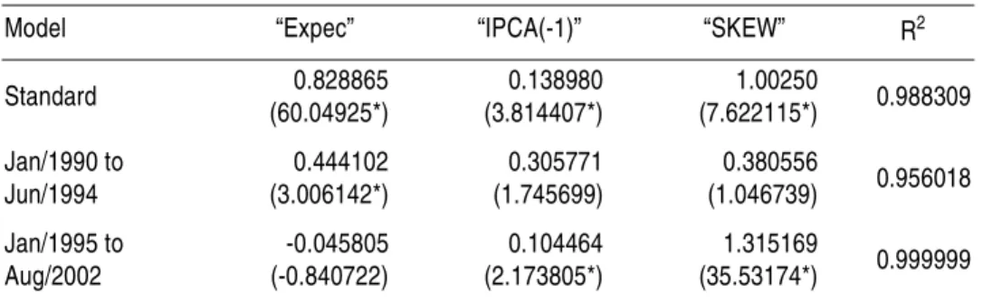
The skewness variable proposed by Mio (2001) is significant in the model. The estimation implies that an one-percentage-point increase in the spread between headline and core produces a variation of 1.03 percentage points in inflation To test for inertia, Mio (2001) proposes that by removing the skewness from both sides of the function, the Curve may be modeled in an equivalent form by “core inflation.” For that, it is necessary that: i) the
-10 0 10 20 08/ 1990 02/ 1991 08/ 1991 02/ 1992 08/ 1992 02/ 1993 08/ 1993 02/ 1994 08/ 1994 02/ 1995 08/ 1995 02/ 1996 08/ 1996 02/ 1997 08/ 1997 02/ 1998 08/ 1998 02/ 1999 08/ 1999 02/ 2000 08/ 2000 02/ 2001 08/ 2001 02/ 2002 08/ 2002 Period La bor Ma rk e t ( % ) -6 -3 0 3 6 9 12 15 In flat ion's For ecast E rr o rs ( % )
asymmetry coefficient in t be indifferent from the unit; and, ii) skewness
la-gged coefficients be symmetric to those of the lala-gged inflation. The LR test performed27 rejects this set of hypotheses (LR = 22.46, for a chi-squared
distribution with two degrees of freedom), and allows us to state that the supply shocks to the Brazilian economy are not responsible for the totality of the inertial component in the analyzed period, with an autonomous res-ponse of inflation to shocks.
It may seem surprising to argue that the rise in inflation after the devaluati-on of the Real, in 1999, was caused by a fall in the NAIRU gap, devaluati-once there was a strong cost pressure on prices. However, Figure A shows that the
SKEW variable captures relative price changes (price asymmetry) caused by
a temporary shock over a few sectors of the economy (tradable goods). Thus, at least part of the exchange rate variation was removed from the esti-mated implicit component. The fall in the NAIRU gap could therefore not be caused by a model’s misspecification that excluded the exchange rate. Three robustness tests were performed with the estimated model. The first consists of the comparison of the values for the expectations coefficients in formulations with different measures of activity. The results showed coeffici-ents with fewer oscillations, even when seasonal componcoeffici-ents are included.28
The greater discrepancies were related to equations that used the unemploy-ment of the metropolitan region of São Paulo (DIEESE) and the industrial production of IBGE. In general, tests reject the hypothesis that the sum of expectations coefficients is equal to the unit.
The second test is the application of the “J” test aiming to verify control va-riables, the seasonal factor of the unemployment and the convexity of the Curve. In the first two cases, the standard model has clear advantage over the alternative, including a model estimated with only adaptive expectati-ons. Conversely, the comparison with the linear model led to inconclusive results. In fact, the latter has good data adjustment, almost equivalent to the standard model, if observed through the R2 of both regressions. What
shar-27 Models used here are available from authors. Note that comparison in this test should not be made on the standard model, as this type of model does not employ lags of the SKEW variable.
ply distinguishes it is the estimated NAIRU’s confidence interval, shown in Graph 5 together with the standard NAIRU.
TABLE F – “J” TEST– COMPONENTS OF THE MODEL – “ENCOM-PASSING”
Note: “Test” reports confronted models, of which the first is a null hypothesis, and the sec-ond the alternative. “Estimated Value” shows the estimation of the alternative model on the test. “t statistics’” informs the significance of the parameter.
GRAPH 5 - COMPARISON OF ESTIMATES - CONVEX AND LINEAR NAIRU
Table G compares two estimations in partial samples, assuming a structural break in July 1994. To improve accuracy, the sampling of the post-Real Plan period began in January 1995. Evidence shows strong sensitivity of the del. The expectations formation changes in comparison with the basic mo-del and between periods. Results of the SKEW variables are also reported.
Test Estimated
value t statistics Choice
Model without control variables X Standard Model 0.926420 4.517390 Standard Model
Model without the “EXPEC” variable X Standard Model 1.005652 24.17325 Standard Model
Model with unemployment seasonality X Standard Model 1.090562 4.030054 Standard Model
Linear Model X Standard Model -0.497429 -0.991702
-3,000 4,000 5,000 6,000 7,000 8,000 9,000 10,000
08/1990 02/1991 08/1991 02/1992 08/1992 02/1993 08/1993 02/1994 08/1994 02/1995 08/1995 02/1996 08/1996 02/1997 08/1997 02/1998 08/1998 02/1999 08/1999 02/2000 08/2000 02/2001 08/2001 02/2002 08/2002
Period
(%)
This sensitivity, however, does not seem to cause problems since the R2
sta-tistics remains very high in every estimation.
TABLE G – ESTIMATION IN PARTIAL SAMPLES
Note: (*) indicates the significance of parameters estimated at 5%.
Finally, Graph 6 compares the NAIRU with results obtained by Portugal and Madalozzo (2000) and Tejada and Portugal (2001), whereas Graph 7 reports the results of Lima (2000).29 While studies that used filters for the
unobservable components revealed an uptrend in the period between the fourth quarter of 1991 and the second quarter of 1993, Portugal and Mada-lozzo (2000) show undefined behavior that lasts until the first half of 1994. When all estimates reach a valley in the first semester of 1995, characteri-zing the implementation of the Real Plan, the NAIRU generated by trans-fer function shows a new increase only in 1996. Another diftrans-ference is the NAIRU gap value presented by the estimates of Tejada and Portugal (2001) and Lima (2000), in the MSR model, in the period that preceded the Real Plan. This result was also obtained in the standard model, however it is not such large as the authors point out. Finally, we should highlight the gap di-fference after the first quarter of 1999, since Lima (2000) points to output loss, as a result of a NAIRU gap larger than the standard model.
Model “Expec” “IPCA(-1)” “SKEW” R2
Standard 0.828865
(60.04925*)
0.138980 (3.814407*)
1.00250
(7.622115*) 0.988309
Jan/1990 to Jun/1994
0.444102 (3.006142*)
0.305771 (1.745699)
0.380556
(1.046739) 0.956018
Jan/1995 to Aug/2002
-0.045805 (-0.840722)
0.104464 (2.173805*)
1.315169
(35.53174*) 0.999999
GRAPH 6 - COMPARING RESULTS - NAIRU IN OTHER STUDIES
GRAPH 7 COMPARING RESULTS NAIRU IN OTHER STUDIES -1990 TO 1999
We analyze now the relationship between Markov regimes and the estima-ted NAIRU. Graphs 8 and 9 combine the smoothed probabilities of the re-gimes with the fundamental characteristics of the Phillips Curve: NAIRU gap and the spread between inflation and expectations. Apparently, there are two different behaviors in the high-inflation period and a third one after the Real Plan. In the months following the Real Plan, the NAIRU gap does not
GRAPH 6 - Comparing Results - NAIRU in Other Studies
4 4,5 5 5,5 6 6,5 7 7,5 8 8,5
1990-4 1991-2 1991-4 1992-2 1992-4 1993-2 1993-4 1994-2 1994-4 1995-2 1995-4 1996-2 1996-4 1997-2
Period
(%)
Unemployment Standard Model Portugal and Madalozzo (2000) Tejada and Portugal (2001)
GRAPH 7 - Comparing Results - NAIRU in Other Studies - 1990 a 1999
4 4,5 5 5,5 6 6,5 7 7,5 8 8,5 9 1990-4 1991-2 1991-4 1992-2 1992-4 1993-2 1993-4 1994-2 1994-4 1995-2 1995-4 1996-2 1996-4 1997-2 1997-4 1998-2 1998-4 1999-2 1999-4 Period (% )
seem to contain important information about the expectations. In fact, in regime 2, there is no systematic error process in the formation of inflation expectations. Therefore, the determination of regimes did not pass through the two stages of demand pressure on inflation. The result should be ascri-bed to the transparency of the government towards the monetary policy, since the correction of the ex-post bias is slow-paced. Thus, the predictabili-ty of monetary policy reduced the “punishment” on agents for maintaining their expectations far from rational.
GRAPH 8 - MARKOVIAN REGIMES AND NAIRU GAP - AUG/90 TO AUG/02
GRAPH 9 - Markovian Regimes and Inflation Error - Aug/90 to Aug/02
0 0.1 0.2 0.3 0.4 0.5 0.6 0.7 0.8 0.9 1 08 /1 9 9 0 08 /1 9 9 1 08 /1 99 2 08 /1 9 9 3 08 /1 9 9 4 08 /1 9 9 5 08 /1 9 96 08 /1 9 97 08 /1 9 98 08 /1 9 99 08 /2 00 0 08 /2 00 1 08 /2 00 2 Period Re g im e Pr o b a b il it y -10 -5 0 5 10 15 In fl a tio n F o re c a s t E rro r (% )
GRAPH 8 - Markovian Regimes and NAIRU Gap - Aug/90 to Aug/02
0 0.1 0.2 0.3 0.4 0.5 0.6 0.7 0.8 0.9 1 08 /19 90 02 /1 9 91 08 /1 9 91 0 2/ 199 2 08 /19 92 02 /19 93 08 /1 9 93 0 2/ 199 4 08 /19 94 02 /19 95 08 /1 9 95 0 2/ 199 6 0 8/ 199 6 0 2/ 199 7 08 /19 97 02 /1 9 98 08 /1 9 98 0 2/ 199 9 08 /19 99 02 /20 00 08 /2 0 00 0 2/ 200 1 08 /20 0 1 02 /20 02 08 /2 0 02 Period R e g im e P ro b a b il it y -1.5 -1 -0.5 0 0.5 1 1.5 2 N A IR U G a p - (% )
R1 R2 R3 NAIRU Gap
On the other hand, the dynamics of hyperinflation has remarkable characte-ristics, as it comprises two different regimes. While, during most of the pe-riod, there was a significant demand gap, expectations remained below the observed inflation. This is the behavior of regime 3, where shocks over the ex-post bias spread almost like a random walk and where inflation is unde-restimated. However, when the gap in activity decreased, its minimum was characterized by regime 1: overestimation of inflation and low persistence of the ex-post bias. So, expectations seemingly anticipated the point where aggregate demand started to pressure inflation again.
In fact, by analyzing the periods where regime 1 coincides with pressures produced by the NAIRU gap we find a correlation with three major events. In mid-1990, the Collor I Plan already showed operational problems, com-pelling the government to unfreeze prices. Worth of note is the permission for the employment contracts to be renegotiated outside the base date, the pressure on the prices of agricultural products, as a result of the harvest yi-eld, and the increase in the manufactured products’ prices, correcting price-freeze distortions. The second period (April to June 1991) stands for repla-cement of the Minister of Finance and generalized disbelief in Collor II Plan. The third phase (November 1991 to January 1992) indicates ortho-dox policies by minister Moreira, who, despite the rise in real interests, sho-cks on public tariffs and exchange rate depreciation, attempted to reorganize public finances and international reserves, respectively. Thus, the effects on the expected inflation rate could not be neglected.
This way, the dynamics proposed by Markov regimes focuses on the future perception of agents about the economy. In the three outlined regimes, it is the future of the economy that determines the perception about inflation. While in regime 2 this perception involved the maintenance of evident mo-netary policies, in regimes 1 and 3, the short-term relationship with the ex-cess aggregate demand determined the reaction of agents to surprises in the economy.
long-term guide, but as a short and medium term indicator that reflects su-pply shocks on the economy. The estimation here considers these factors in-cluding a variable that measures the agents’ behavior on the expectations formation and one that encompasses the effects of short-term shocks on the rate of inflation, in addition to monetary policy corrections. Thus, the un-certainty over the NAIRU should not be seen as a hindrance to the deter-mination of economic policy objectives. As we can observe, the agents assess two major points: monetary policy transparency and demand pressu-res on inflation.
3.4 Monetary Policy Responses Under Partially Rational Expectations
The aim of this section is to test the monetary policy responses in an envi-ronment that presupposes the results heretofore developed and tested. The two hypotheses supporting the formulation are the division of agents throu-gh the expectations formation process; and the incorporation of the Phillips Curve as the kernel of the estimated system. These restrictions are a diffe-rential from literature.30 For Brazil, there are few systems’ estimations with
the same goal. Noteworthy is Minella (2001), who estimates a system with four endogenous variables (prices, output, interest rates and monetary aggregate) between 1975 and 2000. Despite the inclusion of dummy varia-bles, the author’s stratification of sample into three phases was crucial to get consistent results. This section will try to answer the author’s propositions: i) whether monetary policy shocks affect inflation; ii) whether monetary po-licy shocks affect the economic activity; iii) the response of authorities to shocks on inflation and unemployment; iv) the persistence of the inflation; and v) the relationship between money stock and interest rates (MINELLA, 2001, page 5).
The addition of M1 stock growth rate aims at discriminating the behavior of variables in relation to different monetary policy instruments. This is con-sistent with other studies (see PASTORE, 1995, ROCHA, 1997, and MI-NELLA, 2001). Although the variable that controls monetary policy is the primary interest rate, the simulation included M1 to make it similar to
nella (2001). The system uses five endogenous variables: IPCA, EXPEC,
DSELIC, M1-Census and the GAP variable (difference between smoothed
NAIRU and unemployment). SKEW is the exogenous variable. The
inclusi-on of the measure of expectatiinclusi-ons seeks to eliminate the price puzzle from the system, where the positive shock on interest rates increases the price le-vel. This is a common result for US and OECD countries, also reported by Minella (2001) for Brazil. According to Sims (1992), it stems from the ine-xistence of variables that capture expectations, which makes anticipated sho-cks produce an increase in price level.
VAR estimation was sensitive to regime switches. The use of variables to mark economic plans does not cause convergence of impulse-response func-tions, in addition to problems with the residuals. The absence of convergen-ce is a greater problem, sinconvergen-ce there is cointegration between the involved variables. The residual correlation matrix also has simultaneity problems, in-volving the EXPEC, IPCA and ΔSELIC variables. The problem was
recur-rent in all VAR estimations, both through OLS and SUR.31 Thus, the
problem is corrected by imposing an equation with its own dynamics rela-ting at least two of the variables involved. The natural option is for the esti-mated Phillips Curve.32
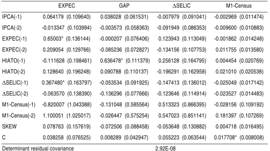
The estimation comprises the period between January 1995 and August 2002, trying to establish comparison with Minella (2001) in the greatest number of characteristics. The model presents two lags in equations in whi-ch IPCA is not an endogenous variable. The LR test points to the model with one lag. However, tests over residuals favored the alternative choice, as shown in Table H. The R2 test, in Table J, shows reasonable adjustment,
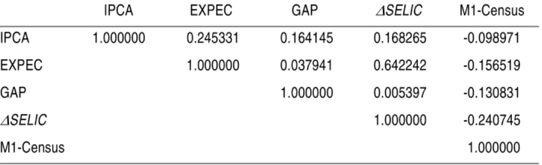
es-pecially with equations whose endogenous variables are monetary policy instruments. Table I shows the correlation of the system’s residuals, where the bad result refers to the relationship between SELIC rate and expectati-ons. The result might probably originate from the proxy’s construction, sin-ce changes to the primary rate may cause contemporaneous changes to the measure.
31 Results of alternative systems, including the full sample, available from authors.
32 We used a slightly different estimation of the curve, incorporating ΔSELIC in the equation, in order